Dimension reduced kernel estimation for distribution function with incomplete data

SUMMARY

This work focuses on the estimation of distribution functions with incomplete data, where the variable of interest Y has ignorable missingness but the covariate X is always observed. When X is high dimensional, parametric approaches to incorporate X — information is encumbered by the risk of model misspecification and nonparametric approaches by the curse of dimensionality. We propose a semiparametric approach, which is developed under a nonparametric kernel regression framework, but with a parametric working index to condense the high dimensional X — information for reduced dimension. This kernel dimension reduction estimator has double robustness to model misspecification and is most efficient if the working index adequately conveys the X — information about the distribution of Y. Numerical studies indicate better performance of the semiparametric estimator over its parametric and nonparametric counterparts. We apply the kernel dimension reduction estimation to an HIV study for the effect of antiretroviral therapy on HIV virologic suppression.

1 Introduction

With advances in technology, high dimensional auxiliary variables or covariates can be collected to augment the incomplete observations in the variable of interest. In surveys, observation of the survey variable is restricted by sampling design, while auxiliary variables are collected prior to sampling to determine the sampling scheme. In clinical trials, observation of the response can be limited due to drop outs, but covariates like baseline characteristics are readily available. Making efficient and reliable use of the auxiliary or covariate information is important.

We consider the incomplete data of a general form

$$(X_i,Y_i,{\delta }_i)i=1,\cdots ,N.$$ (1)

For data with missing response, N is the number of subjects involved, X_i ∈ ℝ^d is the vector of covariates and is always observed, Y_i is the response, δ_i is an indicator with δ_i = 1 if Y_i is observed and δ_i = 0 if otherwise. We will refer to (X_i, Y_i, δ_i) with δ_i = 1 a complete case and δ_i = 0 a nonresponse. According to Little & An (2004), for incomplete data with missing response, efforts should be made to collect all the covariates that predict a nonresponse so that missingness in Y is ignorable (Rosenbaum & Rubin, 1983), i.e.,

$$\mathrm{Pr}(\delta =1\mid Y,X)=\mathrm{Pr}(\delta =1\mid X)=\pi (X).$$ (2)

That is, the chance a subject’s response will be observed is determined by the value of the covariate but not by the response. We will refer to π(X) as the selection probability.

The focus of this paper is the estimation of the distribution function of incompletely observed Y. Naive complete case estimation, i.e., estimating the distribution function using only Y_i’s from complete cases is biased unless Y is missing completely at random. Statistical methods that incorporate covariate information into the distribution estimation of Y fall into two major categories — parametric and nonparametric. A parametric regression estimator, e.g., the model-based estimator (Chambers & Dunstan, 1986) and the modified difference estimator (Rao et al., 1990), assumes a linear regression model of Y versus X. It is consistent and most efficient if the assumed linear relationship is true but not otherwise. There is the Horvitz—Thompson estimator ${\sum }_{i=1}^N\pi {(X_i)}^{-1}{\delta }_i{I}_{[Y_i\le y]}/{\sum }_{i=1}^N\pi {(X_i)}^{-1}{\delta }_i,$, which is consistent if the selection probability is correctly specified but biased otherwise (Särndal et al., 1992). Denote F(y) as the distribution of Y and Q(y ∣ x) as the conditional distribution of Y given X = x. As F(y) = E{Q(Y ∣ X)}, a nonparametric kernel estimator of F(y) is $N^{-1}{\sum }_{i=1}^N\widehat{Q}(y\mid X_i)$ with Q̂(y∣x) the nonparametric kernel estimate of Q(y ∣ x) (Kuk, 1993; Cheng & Chu, 1996). It is consistent with no model specifications, but it is not as efficient as the parametric regression estimators as it uses no model information about Y.

For high dimensional covariates, neither parametric nor nonparametric approaches may work satisfactorily. The parametric approach is hampered by the risk of model misspecification: with high dimensionality in the covariates, it is very hard to check on the relationship between Y and X as well as to find an exactly correct model for the selection probability. The nonparametric kernel estimation is hampered by the curse of dimensionality, as the conditional distribution Q(y∣x) needs to be estimated through a multivariate kernel regression, which suffers the curse of dimensionality and is feasible for d ≤ 5 (Härdle et al., 2004).

We pursue a semiparametric approach. It is built upon a nonparametric estimation framework but utilizing prior model information through a parametric working index for reduced dimension. It consists of two steps. In the parametric step, information contained by X about Y is summarized by a parametric working index S = S(X), a condensation of the covariate information from ℝ^d to ℝ¹. In the nonparametric step, the conditional distribution of Y given the univariate index S, denoted by Q(y∣S), is nonparametrically estimated by univariate kernel regression, and F(y) is estimated by $N^{-1}{\sum }_{i=1}^N\widehat{Q}(y\mid S_i)$ with S_i = S(X_i). With a proper parametric working index, it not only reduces the dimension in nonparametric regression from d to 1, but also improves estimation efficiency by guiding nonparametric regression along a direction that adequately summarizes the covariate information. With nonparametric kernel regression for Q(y ∣ S), it relieves reliance on model specification. We will refer to this semiparametric approach as the kernel dimension reduction (KDR) estimation.

We will describe KDR estimation in section 2. It is shown theoretically in section 3 and numerically in section 4 that KDR estimator has improved robustness over its parametric counterparts and is more efficient than the nonparametric kernel estimator. It relies on minimal prior model information, which is especially attractive for high dimensional data, where model specification and checking is difficult. As an illustration, we apply KDR to an HIV study in section 5. A brief discussion about KDR for survey data is given in section 6.

2 Methodology

Let S : ℝ^d → R be a continuous function, such that S(X) summarizes covariate information about Y. Denote the univariate image as S = S(X). We will discuss the selection of S in the next section. Here, S can be any continuous function. Denote Q(y∣s) as the conditional distribution of Y given S = s. It follows that $N^{-1}{\sum }_{i=1}^{N}Q(y\mid S_i)$ is unbiased estimator of F(y) for any S. However, Q(y ∣ s) is unknown and needs to be estimated. To avoid reliance on model specification, we do not want to assume any parametric form of Q(y ∣ s) but estimate it nonparametrically.

For Q(y ∣ s) = E{I_{[Y ≤y]}∣S = s}, it can be estimated by a nonparametric regression of I_[yi≤y] versus s_i = S(x_i), for example, by the Nadaraya – Watson kernel regression (N-W: Nadaraya (1964) and Watson (1964)). However, the ignorable missingness (2) does not ensure the conditional independence between Y and δ given S. That is, Q(y ∣ s) can be different from Q(y ∣ s, δ = 1), the conditional distribution over the complete cases. Therefore, the N-W kernel estimation of Q(y ∣ s) needs to be modified to

$$\widehat{Q}(y\mid s)=\sum _{j=1}^N\frac{{\delta }_j}{{\pi }_j}{K}_b(s-s_j)I_{[y_j\le y]}/\sum _{j=1}^N\frac{{\delta }_j}{{\pi }_j}{K}_b(s-s_j).$$ (3)

In (3), I(·) is the indication function, π_j = π(x_j), s_j = S(x_j), K_b(u) = b⁻¹ K(u/b), K(·) is the kernel function which is generally a symmetric density function with finite variance, and b is the smoothing bandwidth. Q̂(y ∣ s) can be written as a weighted average ${\sum }_{j=1}^N{\omega }_j(s)I_{[y_j\le y]}$, with

$${\omega }_j(s)=\frac{{\delta }_j}{{\pi }_j}{K}_b(s-s_j)/\sum _{j=1}^N\frac{{\delta }_j}{{\pi }_j}{K}_b(s-s_j)$$

a Horvitz – Thompson (H-T: Horvitz & Thompson (1952)) and N-W combined weight. With H-T weight 1/π_j, it assigns a higher weight to a complete case (s_j, y_j, δ_j = 1) that is less likely to be observed. With N-W weight K_b(s − s_j), it assigns a higher weight to a complete case with s_j closer to s. As shown in the appendix, (3) is consistent for Q(y ∣ s). Furthermore, at any given s, Q̂(y∣s) is a conditional distribution function: it is non-decreasing with Q̂(−∞∣s) = 0 and Q̂(∞∣s) = 1 and right continuous. However, Q̂(y ∣ s) may be not continuous. A continuous version is

$${\widehat{Q}}_c(y\mid s)=\sum _{j=1}^N\frac{{\delta }_j}{{\pi }_j}{K}_b(s-s_j)\mathbf{K}(\frac{y-y_j}{b})/\sum _{j=1}^N\frac{{\delta }_j}{{\pi }_j}{K}_b(s-s_j),$$ (4)

where K is the distribution function of kernel density K. For example, if normal density is used as the kernel, then K is the normal distribution function. It is obvious that (4) is weighted average ${\sum }_{j=1}^N{\omega }_j(s)\mathbf{K}\{(y-y_j)/b\}$, with the only difference from (3) being that the binary function is replaced by the continuous kernel distribution function. The resultant estimators for F(y) are

$$\begin{array}{lll}\widehat{F}(y)& =& N^{-1}\sum _{i=1}^N\widehat{Q}(y\mid S_i),\\ {\widehat{F}}_c(y)& =& N^{-1}\sum _{i=1}^N{\widehat{Q}}_c(y\mid S_i).\end{array}$$ (5)

We will refer to (5) as the KDR estimators for F(y), S the working index function and S = S(X) the working index. For multidimensional X ∈ ℝ^d, (5) are semiparametric estimators as a parametric working index S is involved for summarizing the covariate information and reducing the dimension from d to 1. For univariate X and S = X, (5) reduce to nonparametric kernel estimators. As shown in the appendix, the two estimators in (5) are asymptotically equivalent, and we will use the same notation F̂ unless stated otherwise.

For the selection of bandwidth b in estimating Q(y ∣ s), we will follow a simple bandwidth selection strategy proposed in Silverman (1986) and Kuk (1993). Denote R as the range of working index S, the bandwidth in (3) is chosen as b = R/n with $n={\sum }_{i=1}^N{\delta }_i$. For bandwidth selection in (4), we pre-scale {S_i : δ_i = 1} and {Y_i : δ_i = 1} to be of the same range and estimate the common bandwidth by b = R/n.

3 Asymptotic properties

Asymptotic properties are developed under the regularity conditions in the appendix.

Theorem 1

At any given y, N^1/2 {F̂(y) − F(y)} is asymptotically N (0, σ²(y)) distributed with

$${\sigma }^2(y)=\{F(y)-F^2(y)\}+E[\{\pi {(X)}^{-1}-1\}\{Q(y\mid S)-Q^2(y\mid S)\}].$$

Theorem 1 shows that F̂(y) is consistent for any index S but the choice of the working index affects the efficiency. Intuitively, an index function that adequately summarizes the X — information about Y should lead to good estimation efficiency.

Remark 1

In the asymptotic variance, the first part N⁻¹{F(y) − F²(y)} is the variance of the empirical distribution function with no missingness in Y. The second part N⁻¹ E [(π(X)⁻¹ − 1){Q(y∣s) − Q²(y∣s)}] is the variance due to missingness in Y, and it is zero if π ≡ 1. This second part depends on the selection of index S. If S = Q(y∣X), then

$$Q(y\mid S)=E(I_{[Y\le y]}\mid S)=E\{E(I_{[Y\le y]}\mid X)\mid S\}=Q(y\mid X),$$

and the second part of σ²(y) becomes E [(π⁻¹ − 1){Q(y∣X) − Q²(y∣X)}]. That is, with S = Q(y∣X), it conveys all the X — information about the distribution of Y and leads to the estimation of F(y) with the same efficiency as if the full covariates are used. Such an index gives the optimal efficiency among all possible working indices. In fact, any index S that recovers Q(y∣X), i.e., Q(y∣X) = L(S) for some integrable function L, shares this same efficiency as Q(y∣s) = E{E(I_{[Y ≤y]} ∣ X)∣S} = E{L(S)∣S} = Q(y∣X). Therefore, prior model information about Q(y∣X) should be used in the selection of the working index for improved efficiency.

Theorem 1 shows the robustness of KDR to working index selection. Firstly, any working index leads to consistent estimation. Secondly, to reach optimal efficiency, S does not need to be fully correctly specified for Q(y∣X) but only to grasp the core information about Q(y∣X), and the specification of link L is not crucial.

Remark 2

When taking account of the omitted higher order terms, the asymptotic variance of F̂(y) is N⁻¹ σ²(y) + O{(N²b)⁻¹}, with the higher order term coming from the kernel estimation of Q(y∣s). This higher order term is O(N^−9/5) at the optimal bandwidth for univariate kernel regression and is inversely related to the density of S. For high dimension d, this higher order term diminishes faster than that of the nonparametric kernel estimator, which is of order O{N^{−(d+8)/(d+4)}} at the optimal bandwidth for multivariate kernel regression and is inversely related to the density of X (Ruppert & Wand, 1994). Therefore, KDR leads to improved efficiency over a completely nonparametric kernel estimator.

Remark 3

In most cases, the working index S = S(X; β) involves an unknown parameter vector β. Similarly, the selection probability π(X; α) involves an unknown parameter vector α. KDR estimation has to use the estimated index S = S(X; β̂) and the estimated selection probability π(X; α̂) in (5). We show in the appendix that, with maximum likelihood estimation for β and α, the asymptotic normality in Theorem 1 stays the same.

The above properties are developed with the selection probability correctly specified, which is not always possible. Next, we study the robustness of KDR to misspecification. Denote p(X) as a working model for the selection probability, so π_j is replaced by p(x_j) in (3) and (4).

Theorem 2

The KDR distribution estimator F̂(y) has the following double robustness: (i) when p is correctly specified for the selection probability, F̂(y) is consistent for any working index S; (ii) when p is misspecified for the selection probability, F̂(y) is consistent if the working index S = S(X) can recover Q(y ∣ X) in the sense Q(y ∣ X) = L(S) for some integrable function L.

Consistency under (i) follows from Theorem 1. Under condition (ii), the denominator of Q̂(y ∣ s) in (3) converges almost surely to E{δ/p(X)K_b(s − S)} which equals

$$E\{\pi (X)/p(X)K_b(s-S)\}=E\{\pi (X)/p(X)\mid S(X)=s\}g(s)+O(b^2),$$ (6)

where g(s) denotes the marginal density of the working index S. The numerator converges almost surely to E{δ/p(X)K_b(s − S)I_{[Y ≤y]}} = E{π(X)/p(X)K_b(s − S)Q(y ∣ x)}. With Q(y ∣ x) = L(S), the limit of the numerator becomes

$$E\{\pi (X)/p(X)L(S)K_b(s-S)\}=E\{\pi (X)/p(X)\mid S(X)=s\}L(s)g(s)+O(b^2).$$ (7)

It follows from (6) and (7) that Q̂(y ∣ s) is consistent for Q(y ∣ s), and consequently F̂(y) consistent for F(y).

Based on Remark 1 and Theorem 2, an ideal working index is such that S can recover Q(y ∣ x). With π correctly specified, such an index ensures good efficiency; with π misspecified, such an index ensures consistency. As a special case of recoverable working index, we look for S that approximates Q(y ∣ x) as much as possible. Under ignorable missingness (2), Q(y ∣ x) = Q(y ∣ X, δ = 1) and we can carry out a logistic regression of I_[yi≤y] versus x_i over the complete cases to approximate Q(y ∣ x) = E(I_{[Y ≤y]} ∣ X). As the working index needs only to grasp the core information of Q(y ∣ x), even logistic link is not exactly correct, the working index S = logit⁻¹(X; β̂) can still lead to good performance.

For 0 < α < 1, denote the α-th quantile as ξ_α. The KDR quantile estimator is

$${\widehat{\xi }}_{\alpha }=\inf \{\mathrm{y}\in ℝ:\widehat{\mathrm{F}}(\mathrm{y})\ge \alpha \}$$

The following Theorem gives the asymptotic property of the quantile estimator for continuous distributions. Denote F′ as the first order derivative of F.

Theorem 3

If F′ is continuous at ξ_α with F′ (ξ_α) > 0, then the quantile estimator of ξ_α has an asymptotic normal distribution

$$N^{1/2}\{{\widehat{\xi }}_{\alpha }-{\xi }_{\alpha }\}\to N(0,{\{{\sigma }^2({\xi }_{\alpha })/F^{\prime }({\xi }_{\alpha })\}}^2),$$

where σ²(·) is the variance function in Theorem 1.

Theorem 3 shows that the KDR quantile estimator is consistent for any S; in addition, the working index that gives the most efficient estimation of F(y) around y = ξ_α also leads to the most efficient estimation of ξ_α. Therefore, a working index should be ideally as close to Q(ξ_α∣X) as possible. To find such a working index, we first get a rough estimate of ξ_α from a naive complete case quantile estimation, i.e., ${\widehat{\xi }}_{\alpha ,\mathit{cc}}=\inf \{y\in R:{\sum }_{i=1}^N{\delta }_i{I}_{[y_i\le y]}/{\sum }_{i=1}^N{\delta }_i\ge \alpha \}$. Then fit a logistic regression of I_{[Y ≤ξ̂cc,α]} versus X and let S = logit⁻¹(X; β̂), which is an approximate to Q(ξ_α∣X). We use this working index S to estimate the distribution function by (5) and then ξ_α from F̂.

In conclusion, for incomplete data (1) with ignorable missingness in Y, KDR estimation of F(y) at a given y consists of four steps.

• Step 1Estimate the selection probability π(x), for which the common practice is to fit a logistic regression of δ_i versus x_i over i = 1, ⋯ , N.
• Step 2Find a working index S = S(X), such that S(x) approximates or grasps the core information about the conditional distribution Q(y ∣ x). We can fit a logistic regression of I_[yi≤y] versus x_i as following Theorem 2. Though in the logistic regression, a higher order polynomial of X may lead to better approximation, a logistic regression with linear terms of X works well.
• Step 3Estimate the conditional distribution Q(y ∣ s) by a H-T weighted N-W kernel regression (3) or (4).
• Step 4Estimate F(y) by (5).

4 Simulation studies

In this section, we evaluate the numerical performance of KDR for distribution and quantile estimation. We compare KDR with parametric estimation on robustness and with nonparametric kernel estimation on the effect of dimensionality.

We consider the following estimators: the naive complete case estimator F̂_cc, the model-based estimator F̂_m (Chambers & Dunstan, 1986), the modified difference estimator F̂_dm (Rao et al., 1990), the Horvitz-Thompson estimator F̂_HT, the nonparametric kernel estimator, and KDR estimator F̂ and its continuous version F̂_c. For nonparametric kernel estimation, two estimators are considered: one uses only X₁ out of X = (X₁, …, X_d)^T and estimate F(y) by ${\widehat{F}}_{N.1}(y)=N^{-1}{\sum }_{i=1}^N\widehat{Q}(y\mid X_{1i})$, where Q̂(y∣X₁) is from a univariate kernel regression; the other uses the d-dimensional covariate X and estimate F(y) by ${\widehat{F}}_{N.d}(y)=N^{-1}{\sum }_{i=1}^N\widehat{Q}(y\mid X_i)$, where Q̂(y∣X) is from multivariate kernel regression. For F̂_m, F̂_dm, and KDR estimators, they are all evaluated under the same prior model information, which may be incorrect, that Y is linearly related to covariate X. Thus, in KDR, S = logit⁻¹(X^T β̂) from a logistic regression of I_{[Y ≤y]} versus linear terms of X is used as the working index. The selection probability is assumed as linear logistic and estimated by a logistic regression of δ_i versus linear terms of X_i over i = 1, ⋯ , N, which may or may not be correct.

For distribution estimation, we estimate F(y) at y = ξ_α for α = 1/12, ⋯ , 11/12. For quantile estimation, we estimate ξ_α for α = 1/12, ⋯ , 11/12. We report the bias and the root mean squared error (RMSE) at α = 1/4, 1/2, and 3/4, as well as the average maximum of the absolute error over α = 1/12, ⋯ , 11/12.

In the first simulation, Y_i is generated from a linear model $Y_i=X_i^T\beta +\upsilon (X_i)u_i$ for i = 1, ⋯ , N, with X = (X₁, ⋯ , X₅)^T, β = (1, 2, 3, 2, 1)^T, $\upsilon (X)={(X_1^2+\cdots +X_5^2)}^{1/4}$, and u_i independently from N(0, 1). The covariate X has each component independently from uniform (1, 10). The selection probability is π(X) = exp(X^Tα − 25)/{1 + exp(X^Tα − 25)} with α = (1, ⋯ , 1)^T.

Estimates are presented in Table 1 with 300 datasets, each of sample size N = 500. Here, both the assumed linear relationship between Y and X and the assumed linear logistic model for the selection probability are correct, thus the three parametric estimators, F̂_m, F̂_dm, and F̂_HT, are all of negligible biases. Since the linear relationship between Y and X is true, the regression estimators, F̂_m and F̂_dm, are the most efficient. The KDR estimator is of nearly the same performance as the regression estimators. It is more efficient than F̂_HT as the working index additionally incorporates information about the conditional distribution of Y. The two KDR estimators are very close with the continuous version slightly better. For the two nonparametric kernel estimators, F̂_N.d should be consistent but it is of poor performance due to the curse of dimensionality; F̂_N.1 avoids the curse of dimensionality but at the cost of losing information from the other four covariates, thus ignorable missingness does not hold and the biases are non-negligible. Estimates of the quantiles show the same pattern.

Table 1.

Estimates of F(ξ_α) and ξ_α in the first simulation: the bias, the root mean squared error (RMSE), and the average maximum absolute error.

	$\alpha =\frac{1}{4}$		$\alpha =\frac{1}{2}$		$\alpha =\frac{3}{4}$		Ave.max.
	Bias	RMSE	Bias	RMSE	Bias	RMSE	abs.error
F̂cc	-0.189	0.189	-0.21	0.212	-0.121	0.124	0.225
F̂m	0	0.02	0.007	0.023	0.005	0.02	0.031
F̂HT	-0.062	0.134	-0.047	0.097	-0.019	0.048	0.144
F̂dm	-0.007	0.074	-0.003	0.029	0.003	0.019	0.078
F̂N.1	-0.192	0.192	-0.213	0.215	-0.117	0.12	0.23
F̂N.d	-0.124	0.128	-0.064	0.071	-0.007	0.021	0.134
F̂	-0.012	0.044	-0.001	0.024	0.003	0.02	0.082
F̂c	-0.012	0.042	-0.001	0.025	0.003	0.019	0.081
	$\alpha =\frac{1}{4}$		$\alpha =\frac{1}{2}$		$\alpha =\frac{3}{4}$		Ave.max.
	Bias	RMSE	Bias	RMSE	Bias	RMSE	abs.error
ξ̂cc	7.329	7.359	5.222	5.265	3.669	3.751	9.604
ξ̂m	-0.003	0.779	-0.183	0.69	-0.076	0.726	1.349
ξ̂HT	2.074	4.313	1.125	2.95	0.578	2.957	6.539
ξ̂dm	-0.396	2.514	0.034	0.843	-0.027	0.73	2.893
ξ̂N.1	7.449	7.484	5.255	5.301	3.519	3.605	9.757
ξ̂N.d	3.66	3.739	1.515	1.644	0.274	0.787	6.488
ξ̂	-0.018	1.554	0.063	0.77	-0.031	0.716	3.43
ξ̂c	0.04	1.485	0.059	0.751	-0.026	0.705	3.315

In the second simulation, Y is generated from a nonlinear model Y_i1 = (X_i1 + ⋯ + X_i5)² + υ(X_i)u_i, with the selection probability logit{π(X)} = ∥X∥₂ − 15 and ${\parallel X\parallel }_2={(X_1^2+\cdots +X_5^2)}^{1/2}$. The rest stays the same as in the first simulation. Estimates are presented in Table 2. Since the assumed models for Y versus X and the selection probability are incorrect, the parametric estimators F̂_m, F̂_dm, and F̂_HT are all very biased. The nonparametric kernel estimators perform poorly either due to loss of covariate information in F̂_N.1 or the curse of dimensionality in F̂_N.d. The KDR estimator shows the best performance: though the working index S = logit⁻¹(X^T β̂) is not correctly specified for Q(y ∣ x) in this simulation, it contains enough information about Q(y ∣ x) and leads to negligible biases, i.e., the relative bias of KDR quantile estimates (% bias over the true quantile value) are all below 2%, and good estimation efficiency even with the selection probability incorrectly specified. This last observation demonstrates KDR estimator’s robustness to model misspecification.

Table 2.

Estimates of F(ξ_α) and ξ_α in the second simulation: the bias, the root mean squared error (RMSE), and the average maximum absolute error.

	$\alpha =\frac{1}{4}$		$\alpha =\frac{1}{2}$		$\alpha =\frac{3}{4}$		Ave.max.
	Bias	RMSE	Bias	RMSE	Bias	RMSE	abs.error
F̂cc	-0.221	0.222	-0.318	0.32	-0.237	0.239	0.326
F̂m	-0.208	0.208	-0.215	0.216	-0.031	0.038	0.248
F̂HT	-0.221	0.221	-0.316	0.318	-0.233	0.235	0.323
F̂dm	-0.196	0.197	-0.15	0.153	0.032	0.04	0.218
F̂N.1	-0.216	0.216	-0.295	0.296	-0.2	0.203	0.303
F̂N.d	-0.158	0.161	-0.118	0.123	-0.032	0.039	0.178
F̂	-0.023	0.042	-0.013	0.025	-0.008	0.02	0.085
F̂c	-0.014	0.04	-0.001	0.022	-0.002	0.019	0.086
	$\alpha =\frac{1}{4}$		$\alpha =\frac{1}{2}$		$\alpha =\frac{3}{4}$		Ave.max.
	Bias	RMSE	Bias	RMSE	Bias	RMSE	abs.error
ξ̂cc	342.93	343.99	295.76	297.24	244.49	247.03	376
ξ̂m	243.55	244.11	140.05	141.21	31.9	40.36	312.73
ξ̂HT	340.62	341.71	293.8	295.29	241.26	243.85	373.93
ξ̂dm	205.1	205.94	87.8	89.94	-40.72	50.04	283.65
ξ̂N.1	317.98	319.44	265.27	267.12	206.28	209.62	355.29
ξ̂N.d	160.66	164.23	94.81	98.57	36.26	46.41	223.66
ξ̂	16.66	32.84	10.92	25.9	11.44	30.09	101.3
ξ̂c	5.91	29.82	-0.79	25	2.12	28.4	99.67

In case of very high dimensional covariates, model specification is difficult and model checking is hard. Assuming a linear relationship between Y and X and a linear logistic regression model for the selection probability is a common practice. The two simulations indicate that, when data follows the assumed models, KDR has nearly the same performance as the most efficient parametric regression estimator; when data deviates from the assumed models, KDR is robust to model misspecification. As a semiparametric estimator, it outperforms the nonparametric kernel estimator due to its dimension reduction through a parametric working index. Its advantage over nonparametric kernel estimator is expected to increase with increased dimensionality.

5 An application to HIV study

In project PHIDISA, an HIV clinical trial recently completed in South Africa, two combination antiretroviral (ART) regimens were involved: one contained lamivudine (LAM) and the other contained no LAM (non-LAM). Lamivudine has demonstrated good activity against HIV/HBV coinfection (Dore et al., 1999), but resistance develops when it is used as monotherapy (Matthews et al., 2007). In this study, we investigate the effect of LAM when used in combination with other ART drugs on patients with HIV but no HBV infection.

HIV viral load has been a major endpoint in evaluating the effectiveness of an ART regimen. Certain levels of viral load are of clinical importance. One viral load threshold is 50 copies/mL, and a viral load below 50 copies/mL is generally considered as the standard for an efficacious ART (Hill et al., 2007). For PHIDISA, the threshold for efficaciousness was 400 copies/mL, as a new method was adopted for processing blood samples which led to higher viral load reading than the standard method (Hu et al., 2008). Another viral load threshold is 1500 copies/mL, as it is believed that patients with viral load below 1500 copies/mL are less likely to be infectious (Quinn et al., 2000). We will thus investigate the effect of LAM containing regimen on HIV viral load control with the primary interest on the viral load distribution around these important thresholds.

Around 1300 HIV but not HBV infected patients were involved in PHIDISA. They were randomized to either a LAM containing regimen or a non-LAM containing regimen. Baseline characteristics, e.g. age, gender, weight, location, education, WHO stage, albumin, hemoglobin, platelet, CD4 and HIV viral load, were measured for each patient at randomization. The baseline characteristics constitute the vector of covariates (X). Patients had follow up visits at month 1, 2, 3, and every 3 months till month 18, where the response (Y) — HIV viral load — was measured. There were missing observations in the response, e.g., 18% under non-LAM containing regimen and 15% under LAM containing regimen at month 6. As all baseline characteristics that were considered relevant for predicting nonresponse had been collected, ignorable missingness in the response seems plausible.

We apply KDR estimation to the HIV viral load distribution at y = 50, y = 400, and y = 1500 copies/mL. Estimation is performed within each regimen separately, where the selection probabilities and the working indices are estimated within the respective regimen as ART regimen may affect the missing pattern in Y as well as the conditional distribution of Y given X. At each given time point, denote {(X_r,i, Y_r,i, δ_r,i) : i = 1, ⋯ , N_r} as the observations from the N_r patients under regimen r: r = 1 for LAM containing regimen and r = 0 for non-LAM containing regimen. For viral load distribution estimation under regimen r, the selection probability π_r is estimated by logistic regression of δ_r,i versus linear terms of x_r,i, the working index is taken as $S_{r,i}={\mathrm{logit}}^{-1}(X_{r,i}^T{\widehat{\beta }}_r)$ from a logistic regression of I_[yr,i≤y] versus linear terms of x_r,i, and the KDR estimate of the viral load distribution at y is ${\widehat{F}}_r(y)=N_r^{-1}{\sum }_{i=1}^{N_r}{\widehat{Q}}_r(y\mid S_{r,i})$, where Q_r(y ∣ s) is the conditional distribution of viral load under regimen r and is estimated by H-T weighted N-W regression (4). In this example, exponential density is used as the kernel function, and the bandwidth is selected as described in section 2.

Figure 1 depicts the KDR estimated virologic suppression rates under the non-LAM containing regimen and the LAM containing regimen, as well as the difference between the two regimen (suppression rate under LAM minus that under non-LAM) with 95% confidence bounds from bootstrap. It shows that LAM containing regimen relates to higher virologic suppression rates over month 3 to month 15, indicating a benefit of LAM in viral load suppression. For the viral suppression with respect to 400 and 1500 copies/mL, benefit of LAM appears the most around month 6, which is consistent with clinical experience that ART starts to take effect around 3 months of use and may achieve full potency around month 6. This LAM benefit weakens around month 18, possibly due to the development of LAM resistance.

Figure 1.

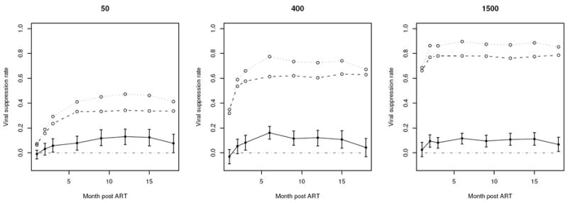
KDR estimated viral suppression rates (viral load ≤ 50, 400, or 1500 copies/mL) over the time: the dotted line is under LAM containing regimen, the broken line is under non-LAM containing regimen, and the solid line is the difference between the two with the 95% confidence bounds.

Next, we look into the viral load magnitude. Since in this clinical trial, viral load assay was subject to a lower detection limit of 50 copies/mL and a high detection limit of 750000 copies/mL, the appropriate magnitude to evaluate is the viral load quantile. Figure 2 depicts the log₁₀ viral load quantiles and the difference in log₁₀ quantiles (log₁₀ quantile under LAM minus that under non-LAM). It shows that LAM containing regimen corresponds to a lower median viral load and lower 90% quantile viral load, indicating its better control of HIV viral load among the moderately and severely diseased patients.

Figure 2.

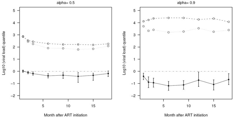
KDR estimated viral load quantile ξ_α at α = 0.5 and 0.9 over the time: the dotted line is the quantile estimate in log₁₀ scale under LAM containing regimen, the broken line is under non-LAM containing regimen, and the solid line is the log₁₀ scale quantile under LAM minus that under non-LAM.

6 Discussion

For the proposed KDR distribution function estimation, we focused on the missing response data, i.e., independent and identically distributed triplets {(X_i, Y_i, δ_i) : i = 1, ⋯ , N}. The same estimation procedure applies to survey data, where the triplets are not independent but with ${\sum }_{i=1}^N{\delta }_i$ equaling some pre-specified survey sample size. Results for survey data were not included in this manuscript. For survey data, the asymptotic normality of Theorem 1 and 3 cannot be easily proved, but we proved the consistency through theory of empirical processes. Simulation studies indicated a similar performance of KDR estimation under survey data as that in section 4.

As a semiparametric estimator, KDR is most appealing for incomplete data with high dimensional covariates: through a parametric working index, it utilizes prior model information to make effective use of the covariate information for reduced dimension and improved estimation efficiency; through nonparametric kernel regression, it attains double robustness to the specification in the selection probability and the parametric working index.

APPENDIX: PROOFS

The asymptotics are developed under the following regularity conditions: (C1) the kernel function K is a symmetric density with ∫ u²K(u)du < ∞; (C2): π(x) is bounded away from 0; (C3) the density of X, denoted by g_x(x), is bounded away from 0 in the support of g_x, so S = S(X) with S continuous has density g(s) bounded away from 0; (C4) ∂Q(y ∣ s)/∂s is bounded in both s and y. As N → ∞, b → 0, Nb³ approaches 0.

A.1 Proof of Theorem 1

We write F̂(y) − F(y) as the sum R_N + S_N + T_N, with

$$\begin{array}{lll}{R}_N& =& N^{-1}\sum _{i=1}^N\{I_{[Y_i\le y]}-F(y)\},\\ S_N& =& N^{-1}\sum _{i=1}^N\{Q(y\mid S_i-I_{[Y_i\le y]}\},\\ T_N& =& N^{-1}\sum _{i=1}^N\{\sum _{j=1}^N{\omega }_j(S_i)I_{[Y_j\le y]}-Q(y\mid S_i)\},\end{array}$$ (A.1)

By the central limit theorem, N^1/2R_N ~ N (0, F(y) − F²(y)) and N^1/2 S_N ~ N (0, E{Q(y∣s) − Q²(y∣s)} By algebraic calculation, we get cov(N^1/2R_N, N^1/2S_N) = −E{Q(y∣s) − Q²(y∣s)}.

Rewrite T_N as T_N = T_1,N + T_2,N with

$$\begin{array}{lll}{T}_{1,N}& =& N^{-1}\sum _{i=1}^N\{\sum _{j=1}^N{\omega }_j(S_i)I_{[Y_j\le y]}-Q(y\mid S_j)\},\\ T_{2,N}& =& N^{-1}\sum _{i=1}^N\{\sum _{j=1}^N{\omega }_j(S_i)Q(y\mid S_j)-Q(y\mid S_j)\}.\end{array}$$ (A.2)

where ${\omega }_j(S_i)=\{N^{-1}\frac{{\delta }_j}{{\pi }_j}{K}_b(S_i-S_j)\}/\{N^{-1}{\sum }_{j=1}^N\frac{{\delta }_j}{{\pi }_j}{K}_b(S_i-S_j)\}$. By the law of large number and the property E{K_b(S − s)} = g(s) + O(b²) with g(s) the density of S at s, $N^{-1}{\sum }_{j=1}^N\frac{{\delta }_j}{{\pi }_j}{K}_b(S_i-S_j)$ converges almost surely to g(S_i) + O(b²) as N → ∞.

Thus

$$\begin{array}{lll}{T}_{1,N}& \simeq & N^{-1}\sum _{i=1}^N{N}^{-1}\sum _{j=1}^N\frac{{\delta }_j}{{\pi }_j}\frac{K_b(S_i-S_j)}{g(S_i)}\{I_{[Y_j\le y]}-Q(y\mid S_j)\}\\ & =& N^{-1}\sum _{j=1}^N\frac{{\delta }_j}{{\pi }_j}\{I_{[Y_j\le y]}-Q(y\mid S_j)\}\{N^{-1}\sum _{i=1}^N{K}_b(S_i-S_j)/g(S_i)\}\\ & \simeq & N^{-1}\sum _{j=1}^N\frac{{\delta }_j}{{\pi }_j}\{I_{[Y_j\le y]}-Q(y\mid S_j)\}.\end{array}$$ (A.3)

The last equation is true as $N^{-1}{\sum }_{i=1}^N{K}_b(S_i-S_j)/g(S_i)\}$ converges almost surely to 1 + O(b²). It is easy to see that $E(\frac{\delta }{\pi }\{I_{[Y\le y]}-Q(y\mid S)\})=0$ and $\mathrm{var}(\frac{\delta }{\pi }\{I_{[Y\le y]}-Q(y\mid S)\})=E({\pi }^{-1}E[{\{I_{[Y\le y]}-Q(y\mid S)\}}^2\mid X])$, where the expectation inside the parentheses equals E (E[{I_{Y ≤y]} − Q(y∣s)}²∣S]∣X) with E[{I_{Y ≤y]}−Q(y∣s)}²∣S] = var(I_{[Y ≤y]}∣S) = Q(y∣s) − Q²(y∣s). It follows that N^1/2T_1,N ~ N (0, E[π⁻¹{Q(y∣s) − Q²(y∣s)}]). Similar derivation shows that T_2,N = o_p(N⁻²). Theorem 1 thus follows from the asymptotic normality of R_N, S_N, and T_N.

For the continuous KDR estimator, F̂_c(y) − F(y) can be written the same as in (A.1) and (A.2) except that T_1,N changes to

$$T_{1,N}^{\ast }=N^{-1}\sum _{i=1}^N\{\sum _{j=1}^N{\omega }_j(S_i)\mathbf{K}(\frac{y-Y_i}{b})-Q(y\mid S_j)\}.$$

Following the same derivation for T_1,N, we have

$$T_{1,N}^{\ast }\simeq N^{-1}\sum _{j=1}^N\frac{{\delta }_j}{{\pi }_j}\{\mathbf{K}(\frac{y-Y_j}{b})-Q(y\mid S_j)\}.$$ (A.4)

As $E\{\mathbf{K}(\frac{y-Y}{b})\}=F(y)+O(b^2)$, it follows that $E(T_{1,N}^{\ast })=E\{\mathbf{K}(\frac{y-Y}{b})-Q(y\mid S\}=O(b^2)$. For the variance of $T_{1,N}^{\ast }$,

$$\begin{array}{lll}N\mathrm{var}(T_{1,N}^{\ast })& =& E[\frac{\delta }{{\pi }^2}{\{\mathbf{K}(\frac{y-Y}{b})-Q(y\mid S)\}}^2]\\ & =& E\left[{\pi }^{-1}E\{{\mathbf{K}}^2(\frac{y-Y}{b})-2Q(y\mid S)\mathbf{K}(\frac{y-Y}{b})+Q^2(y\mid S)\mid X\}\right]\\ & =& E\left({\pi }^{-1}E[E\{{\mathbf{K}}^2(\frac{y-Y}{b})\mid S\}-2Q(y\mid S)E\{\mathbf{K}(\frac{y-Y}{b})\mid S\}+Q^2(y\mid S)]\mid X\right),\end{array}$$

where $E\{{\mathbf{K}}^2(\frac{y-Y}{b})\mid S=s\}=Q(y\mid s)+O(b^2)$ and E{K((y − Y)/b) ∣ s} = Q(y ∣ s)+O(b²) with K a symmetric density. Thus $N\mathrm{var}(T_{1,N}^{\ast })=E[{\pi }^{-1}\{Q(y\mid S)-Q^2(y\mid S)\}]=N\mathrm{var}(T_{1,N})$. It follows that N^1/2{F̂_c(y) − F(y)} follows the asymptotic normal distribution in Theorem 1.

A.2 Proof of Remark 3

For the KDR estimator F̂_π̂(y) with estimated selection probability π̂ = π(X; α̂),

$${\widehat{F}}_{\widehat{\pi }}(y)-\widehat{F}(y)=N^{-1}\sum _{j=1}^N\{\sum _{i=1}^N{W}_{\widehat{\pi },j}(S_i)-W_j(S_i)\}{I}_{[Y_j\le y]}$$

where $W_{\widehat{\pi },j}(S_i)=N^{-1}\frac{{\delta }_j}{{\widehat{\pi }}_j}{K}_b(S_i-S_j)/N^{-1}{\sum }_{j=1}^N\frac{{\delta }_j}{{\widehat{\pi }}_j}{K}_b(S_i-S_j)$, π_j = π(X_j), and π̂ = π(x; α̂) = π + ∂π^T/∂α(x; α)(α̂ − α) by Taylor’s approximation. The denominators of both W_π̂,j(s) and W_j(s) converge to g(s) + O(b²). Thus

$$\begin{array}{lll}{\widehat{F}}_{\widehat{\pi }}(y)-\widehat{F}(y)& =& N^{-1}\sum _{j=1}^N{N}^{-1}\{\sum _{i=1}^N(\frac{{\delta }_j}{{\widehat{\pi }}_j}-\frac{{\delta }_j}{{\pi }_j})K_b(S_i-S_j)/g(S_i)\}{I}_{[Y_j\le y]},\\ & =& \left(N^{-1}\sum _{j=1}^N\frac{{\delta }_j}{{\pi }_j^2}({\pi }_j-{\widehat{\pi }}_j)I_{[Y_j\le y]}\{N^{-1}\sum _{i=1}^N\frac{K_b(S_i-S_j)}{g(S_i)}\}\right)\{1+o_p(1)\}\\ & =& \left(N^{-1}\sum _{j=1}^N\frac{{\delta }_j}{{\pi }_j^2}{I}_{[Y_j\le y]}\frac{\mathit{\partial }{\pi }^T}{\mathit{\partial }\alpha }(X_j;\alpha )(\widehat{\alpha }-\alpha )\right)\{1+o_p(1)\}.\end{array}$$

Since α̂ − α = O_p(N^−1/2) from maximum likelihood estimation in α, it follows that F̂_π̂(y) − F̂(y) = o_p(N^−1/2) and F̂_π̂(y) is of the same asymptotic distribution as F̂(y) in Theorem 1. The proof for the KDR estimation under the estimated working index is similar.

A.3 Proof of Theorem 2

The proof is similar to that of Cheng & Chu (1996). Denote Ψ for the distribution function of N^1/2(ξ̂_α − ξ_α). At any given t, Ψ(t) = P{N^1/2(ξ̂_α − ξ_α) ≤ t} = P(ξ̂_α ≤ ξ_α + N^−1/2t). Denote ξ_α,N = ξ_α + N^−1/2t, then

$$\begin{array}{lll}\mathrm{\Psi }(t)& =& P\{\widehat{F}({\widehat{\xi }}_{\alpha })\le \widehat{F}({\xi }_{\alpha ,N})\}\\ & =& P\{\alpha \le \widehat{F}({\xi }_{\alpha ,N})\}\\ & =& P\left(\frac{N^{1/2}\{\alpha -F({\xi }_{\alpha ,N})\}}{\sigma ({\xi }_{\alpha ,N})}\le \frac{N^{1/2}\{\widehat{F}({\xi }_{\alpha ,N})-F({\xi }_{\alpha ,N})\}}{\sigma ({\xi }_{\alpha ,N})}\right)\\ & =& 1-\mathrm{\Phi }\left(\frac{N^{1/2}\{\alpha -F({\xi }_{\alpha ,N})\}}{\sigma ({\xi }_{\alpha .N})}\right)\end{array}$$

By Taylor’s approximation, α − F(ξ_α,N) = −F′(ξ_α)N^−1/2t + O(N⁻¹). From Lebesgue dominated convergence theorem, σ(ξ_α,N) → σ(ξ_α). Thus, N^1/2{α − F(ξ_α,N)}/σ(ξ_α,N) → −F′(ξ_α)t/σ(ξ_α). Therefore $\mathrm{\Psi }(t)=1-\mathrm{\Phi }\left(-\frac{F^{\prime }({\xi }_{\alpha })t}{\sigma ({\xi }_{\alpha })}\right)=\mathrm{\Phi }\left(\frac{t}{\sigma ({\xi }_{\alpha })/F^{\prime }({\xi }_{\alpha })}\right)$ and Theorem 2 follows.

References

- Chambers RL, Dunstan R. Estimating distribution functions from survey data. Biometrika. 1986;73:597–604. [Google Scholar]
- Cheng PE, Chu CK. Kernel estimation of distribution functions and quantiles with missing data. Statistica Sinica. 1996;6:63–78. [Google Scholar]
- Dore GJ, Cooper DA, B C. Dual efficacy of lamivudine treatment in human immunodeficiency virus/hepatitis b virus coinfected persons in a randomized, controlled study (caesar) Journal of Infectious Diseases. 1999;180:607–613. doi: 10.1086/314942. [DOI] [PubMed] [Google Scholar]
- Härdle W, Müller M, Sperlich S, Werwatz A. Nonparametric and semiparametric models. Berlin Heidelberg: Springer-Verlag; 2004. [Google Scholar]
- Hill A, Miralles D, Vangeneugden T. Should we now adopt the hiv-rna < 50 copy endpoint for clinical trials of antiretroviral-experienced as well as naive patients? AIDS. 2007;21:1651–1653. doi: 10.1097/QAD.0b013e3282703593. [DOI] [PubMed] [Google Scholar]
- Horvitz DG, Thompson DJ. A generalization of sampling without replacement from a finite universe. Journal of American Statistical Association. 1952;47:663–685. [Google Scholar]
- Hu Z, Follmann D, Qin J, Dewar RL, Sangweni P. A nonparametric likelihood test for detecting discordance between two measurements with application to censored viral load determinations. Statistics in Medicine. 2008;27:795–809. doi: 10.1002/sim.3298. [DOI] [PMC free article] [PubMed] [Google Scholar]
- Kuk AYC. A kernel method for estimating finite population distribution functions using auxiliary information. Biometrika. 1993;80:385–392. [Google Scholar]
- Little R, An H. Robust likelihood-based analysis of multivariate data with missing values. Statistica Sinica. 2004;14:949–968. [Google Scholar]
- Matthews GV, Bartholomeusz A, Locarnini S, Ayres A, Sasaduesz J, Seaberg E, Cooper DA, Lewin S, Dore GJ, Thio CL. Characteristics of drug resistant hbv in an international collaborative study of hiv-hbv-infected individuals on extended. AIDS. 2007;20:863–870. doi: 10.1097/01.aids.0000218550.85081.59. [DOI] [PubMed] [Google Scholar]
- Nadaraya EA. On estimating regression. Theory of probability and its application. 1964;9:141–142. [Google Scholar]
- Quinn TC, Wawer WJ, Sewankambo N. Viral load and heterosexual transmission of human immunodeficiency virus type 1. New England Journal of Medicine. 2000;342:921–929. doi: 10.1056/NEJM200003303421303. [DOI] [PubMed] [Google Scholar]
- Rao JNK, Kovar JG, Mantel HJ. On estimating distribution functions and quantiles from survey data using auxiliary information. Biometrika. 1990;77:365–375. [Google Scholar]
- Rosenbaum PR, Rubin DB. The central role of the propensity score in observational studies for causal effects. Biometrika. 1983;60:211–213. [Google Scholar]
- Ruppert D, Wand MP. Multivariate locally weighted least squares regression. Annals of Statistics. 1994;22:1346–1370. [Google Scholar]
- Särndal C, Swensson B, Wretman J. Model assisted survey sampling. New York: Springer-Verlag; 1992. [Google Scholar]
- Silverman BW. Density estimation for statistica and data analysis. London: Chapman and Hall; 1986. [Google Scholar]
- Watson GS. Smooth regression analysis. Sankhya. 1964;26:359–372. [Google Scholar]