A Parameter Estimation Technique for Stochastic Self-Assembly Systems and Its Application to Human Papillomavirus Self-Assembly

Abstract

Virus capsid assembly has been a key model system for studies of complex self-assembly but does pose some significant challenges for modeling studies. One important limitation is the difficulty of determining accurate rate parameters. The large size and rapid assembly of typical viruses make it infeasible to directly measure coat protein binding rates or infer them from the relatively indirect experimental measures available. In the present work, we develop a computational strategy to infer coat-coat binding rate parameters for viral capsid assembly systems by fitting stochastic simulation trajectories to experimental measures of assembly progress. Our method combines quadratic response surface and quasi-gradient-descent approximations to deal with the high computational cost of simulations, stochastic noise in simulation trajectories, and limitations of the available experimental data. The approach is demonstrated on a light scattering trajectory for a human papillomavirus (HPV) in vitro assembly system, showing that the method can infer rate parameters that produce accurate curve fits and are in good concordance with prior analysis of the data. These fits provide insight into potential assembly mechanisms of the in vitro system and a basis for exploring how these mechanisms might vary between in vitro and in vivo assembly conditions.

1. Introduction

Virus capsid assembly has been a key model system for understanding the principles of complicated molecular self-assembly systems [1, 2]. Simulation studies have been central to these efforts, providing a way to study emergent properties and conduct in silico experiments that would be infeasible in practice and intractable to analyze theoretically. For example, simulation studies have made it possible to infer emergent properties of different hypothetical models of assembly [3–6], explore effects of parameter variations on assembly progress [5, 7–9], and examine details of reaction pathways and assembly mechanisms implied by theoretical models of assembly [7, 10–13]. There are, however, substantial obstacles to successful use of simulation methods, one of the most important being the need for accurate parameters of assembly. For capsid assembly, these parameters would typically correspond to rates of reactions involved in assembly or disassembly of coat proteins. While estimates of free energies of binding have been derived for some viruses [14, 15], precise rate constants for coat-coat binding are not known for any real virus system. This limitation has led to studies typically either assuming literature-derived “best guesses” for unknown parameters [16], attempting to infer approximate rate parameters from structural models [17, 18], or scanning parameter spaces to identify the range of possible behaviors available to a viral system [5, 6, 8, 9, 13, 19, 20]. Such simulation studies have, however, suggested that relatively small changes in parameters can lead to large changes in assembly mechanisms [13], calling into question how much one can learn about any particular virus from models with even well constrained parameter values. For simulations of capsid assembly to move from generalities about ranges of possible behaviors to predictive models of particular viruses will require new methods to learn the rate parameters underlying actual viral assembly systems.

Fortunately, simulation methods used to study capsid assembly in the abstract also in principle provide one a mechanism for learning parameters consistent with any given experimental measure of assembly progress. Generally, estimation of parameters in a computational or mathematical model of a system of interest is posed as an optimization problem. The goal of this optimization is to minimize an objective function $f\left(\overrightarrow{p}\right)$ that measures deviation between simulated and real assembly data with respect to the vector of parameters $\overrightarrow{p}$. While many generic optimization methods can in principle be applied to such problems, the appropriate methods for any particular system will depend on many characteristics of the system to be fit. Virus assembly systems present several special challenges to optimization approaches to parameter fitting. Individual simulations, and hence objective function evaluations, are often computationally costly; a single trajectory can require days or weeks of compute time to model the time scale of a typical assembly reaction. Furthermore, these computational costs can change rapidly with parameter values. In addition, simulations of more complicated virus models are usually conducted with stochastic methods (either stochastic simulation algorithm (SSA) models [18, 21] or Brownian dynamics and related particle models [5–7, 9, 22]), making it difficult to accurately evaluate the objective function and, even more so, to evaluate the derivatives needed for most optimization methods.

Since we lack closed form expressions for non-trivial models of capsid assembly, the parameter fitting problem falls under the class of simulation optimization, where the objective function needs to be evaluated through a simulation [23]. Reviews on the methods used for optimization of stochastic simulation systems can be found elsewhere [23–27]. Optimization algorithms for stochastic systems (for example, quasi-gradient methods and algorithms of type Keifer-Wolfowitz) do not directly deal with the gradient of the objective function due to the errors introduced in the gradient estimates because of the noise embedded in such systems. Various techniques have been developed to approximate gradients in these methods, such as specialized finite difference schemes and infinitesimal perturbation analysis. These techniques, however, may impose restrictive conditions on the form of the potential surface to be fit. Another important class of method is response surface methodology, which fits a smoothed regression model to the potential surface and optimizes relative to the regression model. The minimum of the fitted function is then estimated to be the minimum of the search space [26]. Though the number of simulations required for optimization by such a procedure is reduced compared to gradient-based methods, response surface methods can perform poorly when the metamodel is not a good approximation of the search space, the search space is inadequately sampled, or the search space is characterized by very sharp ridges and large valleys with nearly zero curvatures [26, 28].

In the present work, we develop a computational strategy for parameter fitting of capsid assembly systems designed to deal with the particular computational challenges capsid assembly systems present. The method interpolates between response surface and quasi-gradient approximations to provide fast handling of smooth regions of the objective function with robust handling of more difficult regions. We specifically develop the method for use with light scattering data, a widely used approach for monitoring in vitro capsid assembly systems [29], although the algorithm is generic with respect to the data used. We demonstrate the approach on a problem of fitting rate parameters to light scattering data from a human papillomavirus (HPV) in vitro assembly system [30]. We show that the method can achieve a good quality fit to the real data that shows moderate sensitivity to uncertainty in the estimates or the experimental data. This parameter fit further provide specific suggestions about mechanisms of assembly of the HPV in vitro system. The work provides a first step towards using prevailing coarse-grained models of capsid assembly to make inferences about assembly mechanisms for specific viruses and about how these mechanisms might be altered under different assembly conditions or hypothetical experimental or therapeutic interventions.

2. Materials and methods

Our parameter fitting method relies on a local optimization algorithm combined with various heuristics to approximate a global parameter search. The method is applied to fit a coarse-grained stochastic model of capsid assembly to light scattering data tracking average progress over time of an HPV in vitro assembly system. This section first presents the local optimization algorithm, followed by an overview of the data and simulation methods used to evaluate the objective function, then a description of how these methods are embedded in a heuristic global search, and finally details on the implementation of the methods and execution of the validation study performed here.

2.1. Local Optimization Algorithm

At a high level, our local optimization algorithm proceeds in five basic steps. First, it conducts a set of simulations on a grid surrounding the current best guess as to the optimum, with individual grid points corresponding to small variations in the parameters to be fit, and measures the objective value at each point. Second, it generates a quadratic response surface regression model for the potential surface and uses the minimum of the quadratic model to estimate the minimum of the objective function in the region of the current best guess. Third, it uses a subset of the evaluated parameter values to estimate the gradient near the best guess. Fourth, it creates an interpolated inference between a gradient descent step and the response surface minimization, with the degree of interpolation dynamically adjusted based on prior steps of the algorithm. Fifth, it tests the objective value at the predicted optimum and selects a new best guess and grid spacing, which also controls the degree to which the method favors the quasi-gradient or the response surface predictions. Depending the quality of improvement over preceding steps, it either returns to step one for further processing or terminates and returns a solution. Figure 1 provides pseudocode for the overall algorithm.

Figure 1.

Pseudocode for the local optimization algorithm.

Given an initial guess and a step size, the method begins by defining a neighborhood (a grid of points around the initial guess) and using simulations to calculate the value of the objective function at a subset of the grid points. In each case, the subset of possible perturbations around the prior best guess was chosen somewhat arbitrarily to provide sufficient points to fit a quadratic interpolant without producing an exponential blowup of the number of points used in the number of parameters. The selection of a subset is needed because the number of points required to fit the interpolant grows only quadratically with the number of parameters to be fit, while the number of perturbations a fixed distance in a subset of the dimensions will grow exponentially in the number of parameters. For two-parameter searches, simulations are run at the center of the grid (i.e., the previous best guess) and values of ±1/s for each parameter, producing a total of nine points. For three parameter searches, simulations were conducted for the center of the grid, for variations of ±1/s in any one parameter, and for a subset of combinations of variations in two parameters corresponding to ±1/s in the first and either second or third parameter. This produced a total of fifteen points. For four-parameter searches, we used the center point, all single parameter variations of ±1/s, variations of all pairs of points by ±1/s, and simultaneous increase or simultaneous decrease of all parameters by 1/s. This set produced a total of 21 data points. Details of the objective function evaluation are described in Section 2.2 below. Conducting these simulations is the most computationally intensive step of the optimization and we therefore run the individual simulations at this stage in parallel to reduce the total compute time.

The method next uses a quadratic interpolant to fit a response surface to the set of simulated grid points. For any given parameter set, we fit a polynomial consisting of a constant term and all linear and quadratic terms in each variable. For example, for a search of two parameters x₁ and x₂, we fit a set of coefficients c₀, … , c₅ for the following equation:

$$f\approx c_0+c_1{x}_1+c_2{x}_2+c_3{x}_1^2+c_4{x}_1{x}_2+c_5{x}_2^2.$$

For three parameters, the equation takes the form

$$f\approx c_0+c_1{x}_1+c_2{x}_2+c_3{x}_3+c_4{x}_1^2+c_5{x}_1{x}_2+c_6{x}_1{x}_2+c_6{x}_1{x}_3+c_7{x}_2^2+c_8{x}_2{x}_3+c_9{x}_3^2$$

and for four parameters, the equation takes the form

$$\begin{array}{cc}\hfill & f\approx c_0+c_1{x}_1+c_2{x}_2+c_3{x}_3+c_4{x}_4+c_5{x}_1^2+c_6{x}_1{x}_2+c_7{x}_1{x}_3+c_8{x}_1{x}_4+c_0{x}_2^2+\hfill \\ \hfill & c_{10}{x}_2{x}_3+c_{11}{x}_2{x}_4+c_{12}{x}_3^2+c_{13}{x}_3{x}_4+c_{14}{x}_4^2.\hfill \end{array}$$

In each case, the fitting is performed through least-squares polynomial regression. We use a quadratic interpolant because it simplifies the problem of optimizing the parameters with respect to the response surface; the minimum value of a quadratic interpolant on a bounded region must occur either at a unique minimum point of the paraboloid or at a boundary of the region. We find the optimum among those possibilities through a call to the Matlab simulannealbnd routine. The minimum value of the fitted curve provides the response surface estimate of the optimal parameter set. We subtract the current best guess from this estimate to obtain an offset to the response surface estimate.

The method then uses a subset of the grid points to estimate the gradient of the objective function. The partial derivative with respect to each parameter is estimated by a second-order finite difference approximation:

$$\frac{\partial f}{\partial g_i}\approx \frac{f(g_1,\dots ,g_i+\frac{1}{s},\dots ,g_k)-f(g_1,\dots ,g_i-\frac{1}{s},\dots ,g_k)}{2∕s}$$

where k is the total number of parameters to be fit. The full vector of partial derivatives is normalized to unit length.

The two guesses, corresponding to the quadratic fit and the gradient descent, are then interpolated to produce an estimated parameter change for the next step of the simulation. We combine the offset to the response surface fit $\overrightarrow{h}$ and the estimated normalized gradient ▽f with the formula

$$(\overrightarrow{h}-s\nabla f)∕(s^2+1).$$

This formula has the effect of producing an interpolant that will approximate the response surface fit for small s and approximate a quasi-gradient descent step for large s, with the length of the step decreasing with increasing s. The formula is designed to allow for dynamic adjustment towards short gradient steps in difficult regions of parameter space and towards larger steps and quadratic fits in more smoothly varying regions of parameter space. In this regard, it is similar to a Levenberg-Marquardt [31, 32] optimization strategy.

The final step of the algorithm consists of evaluating the newly generated candidate point and adjusting the current estimate and grid size appropriately. The method conducts additional objective function evaluation at the interpolated point. In order to minimize stochastic error in this final estimate, the algorithm runs repeated trajectories until the standard error in the estimated RMSD is below 10% of the mean estimated RMSD. If this estimate indicates that the method succeeded in reducing the objective function then the next point is selected as the starting point for the next round of grid generation and the scaling parameter s is reduced by half. If the newly generated point is a poorer approximation, then the parameter s is doubled and the algorithm conducts a new search with the previous starting point. We terminate the local search if s is increased to 512 without producing any local improvement.

2.2. Evaluating the Objective Function

Our method optimizes with respect to the deviation between an experimental measure of progress of an assembly system and a simulation of that measure for a defined parameter set. For the present purposes, we use light scattering data, a standard measure of progress of in vitro capsid assembly systems [29] that corresponds approximately to average assembly size versus time. These data are matched to simulations conducted with a stochastic simulation algorithm [33] simulator developed to model self-assembly using local rules principles [4].

The experimental data for this study was taken from multi-angle light scattering (MALS) measurements of HPV assembly. The data was presented in Casini et al. [30] and kindly provided by David Wu. The data consists of Rayleigh ratios as functions of time for purified HPV LP1 coat protein assembled in vitro. Rayleigh ratios are parameterized by scattering angle, θ, and are approximately related to the weight-average molecular weight of assemblies in a solution by the following equation:

$$R\left(\theta \right)=\left(Kc\right)\left[M_{w}P\right(\theta )-2A_{2}c{M}_w^2{P}^2(\theta \left)\right].$$

Here, K is a global scaling constant, c is the mass concentration of the proteins in solution, M_w is the weight-average molecular weight (g mol⁻¹), P(θ) is a parameter called the form factor defined by protein shape, and A₂ is the second virial coefficient (a scaling constant for the second-order term in the approximation) (mol ml g⁻²). The most common use of such data is to measure turbidity, where θ is fixed to 90°, as in the present study. We selected one specific data set from those measured in Casini et al. for our validation, corresponding to assembly at 145μg ml⁻¹. This curve was chosen because comparison between the measured peak light scattering and theoretical projections suggested it went closest to completion of any of the conditions they examined.

Simulated data is generated using simulations based on a kinetic local rule model [5], which describes the assembly process in terms of elementary subunits that bind to one another through pairwise interactions described by local rule sets [4]. Papillomavirus coat proteins tightly associate into pentameric capsomers in vitro that are maintained even if the capsid is depolymerized [34]. We therefore chose to treat capsomers as the basic assembly subunit rather than coat monomers as in our prior work. We constructed two rules describing the pairwise interactions between capsomers in the HPV structure. Figure 2 shows the two rules, for capsomers in pentameric and hexameric binding environments, a screen snapshot of the complete structure they produce, and an expanded region of the complete structure labeled to illustrate the mapping of bond types to the structure. There are four distinct binding interactions possible (labeled A-D in the figure). Interaction type A corresponds to an asymmetric interaction between a pentameric and a hexameric binding site, B and C to two distinct asymmetric interactions between pairs of hexameric binding sites, and D to the symmetric interaction of two instances of a common hexameric binding site. A simulation is parameterized by an on- and an off-rate for each of these four kinds of interactions. For purposes of the simulation, we assumed each capsomer had a defined binding configuration (pentameric or hexameric) and did not allow switching between them. All simulations were conducted with stoichiometric amounts of the two configurations, 1200 pentameric and 6000 hexameric capsomers, sufficient to produce 100 complete capsids.

Figure 2.

Local rule model for papillomavirus assembly from capsomers. (a) A set of two local rules describing the binding interactions of pentameric and hexameric capsomers. Binding sites are labeled by a bond type (A-D), with subscripts “+” and “−” used to denote the two complementary binding sites for a pairwise interaction and “0” to denote the single site involved in a symmetric type D interaction. (b) Screen snapshot of a single simulated capsid generated from the local rules of part (a). (c) Expanded view of a region of the snapshot highlighting an example of each bond type (circled letters A-D) and the two contributing binding sites for each (labeled “+,” “−,” or “0”).

Simulations were conducted using a discrete event self-assembly simulator described in prior work [10, 21]. The simulator implements a stochastic simulation algorithm (SSA) [33] simulation of the pathway set implied by the set of local rules. At each step of a simulation, either one bond is formed from two unpaired binding sites consistent with the local rules or one existing bond is broken. As in our prior work, simulations explicitly disallowed breaking of “loops” of bound particles in multiply-connected structures. In addition, bonds were allowed to form only at ideal intersubunit angles, preventing the creation of malformed structures. Readers are referred to our prior work for detailed information on the simulation model and algorithms. The output of a simulation consists of a time trajectory describing the numbers of structures of each possible size as a function of time over the course of a simulation. Simulations were cut off at 300 minutes of simulated time regardless of their state of completeness at that time. Note that this amount of simulated time can correspond to a widely varying amount of compute time, ranging from hours to days per trajectory depending on the specific simulation parameters.

Each simulation output was then converted to a simulated light scattering curve. Following Casini et al. [30], we assumed the second order coefficient for the Raleigh curve would be negligible for protein assemblies at the concentrations under consideration. We therefore transformed the simulator output into a simulated Rayleigh ratio using the following equation:

$$R\left(\theta \right)=Kc{M}_w,$$

where

$$M_w=\frac{\sum _i{n}_i{M}_i^2}{\sum _i{n}_i{M}_i}.$$

Here, n_i is the number of assemblies of size i and M_i is the molecular weight of the assembly of size i, derived from a capsomer molecular weight of 250 kDa.

Finally, we derived an objective function corresponding to the root mean square deviation (RMSD) between the true and simulated light scattering curves:

$$f(\overrightarrow{p},t)=\frac{\sqrt{\frac{1}{t}{\int }_t{\left[R_{\mathit{sim}}(\theta ,\overrightarrow{p},t)-R_{\mathit{exp}}(\theta ,t)\right]}^2}}{\sqrt{\frac{1}{t}{\int }_t{\left[R_{\mathit{exp}}(\theta ,t)\right]}^2}}$$

where $R_{\mathit{sim}}(\theta ,\overrightarrow{p},t)$ is the simulated Rayleigh ratio obtained for time t and parameter vector $\overrightarrow{p}$. R_exp(θ, t) represents the corresponding experimental data point. It is to be noted that our choice of the objective function also reflects our implicit assumption of Gaussian noise embedded in the response of the system. The function $f(\overrightarrow{p},t)$, evaluated for a given parameter set $\overrightarrow{p}$ and for t = 195.35 min (corresponding to the full time course of the real data set) provides the objective function for parameter optimization. Note that we optimize over log rates, rather than raw rates, so that grid spacing corresponds to multiplicative rather than additive variation in rate constants.

2.3. Heuristic Global Optimization

The algorithm described in section 2.1 provides a general scheme for local optimization in the neighborhood of some initial guess as to the parameter values. We would ideally prefer a global optimization over all possible values, but we cannot guarantee global optimality in the absence of strict constraints on the objective function and its derivatives that are unavailable for our simulations. We therefore use a heuristic strategy that does not guarantee global optimality. The strategy depends on starting with a scan of a reduced parameter space to find a good starting point for local search, followed by successive expansions of the parameter set as local optima are found for reduced parameter sets. The intuition behind the method is that optimal binding parameters will be sufficiently similar to one another that the best fit derived from the reduced space will provide a sufficiently good guess for local optimization in the increased space.

We begin the search in a two-parameter space that assumes a single on-rate and a single off-rate shared by all interaction types. We start the search in this initial two-parameter space by evaluating the objective function at a set of regularly spaced grid points corresponding to parameter variations in that space. For the present work, we computed a total of twenty objective values corresponding to on-rates of 1.04×10¹ to 1.04×10⁵ M⁻¹s⁻¹ in 10-fold increments and off-rates rates of 1.67×10⁻² to 1.67×10¹ s⁻¹ in 10-fold increments. These ranges were chosen, based on prior studies of a model of T=1 assembly [13], to cover a broad space of possible pathways in a biologically plausible region of the parameter space. We then select the point with minimum objective value as the initial guess for a two-parameter local optimization using the algorithm of section 2.1. The scaling parameter s is initially set to a ten-fold variation.

We then hold the inferred off-rate fixed for subsequent simulations and allow on-rates to differ between bond types. The next step of optimization allows for two on-rates: one for pentameric-hexameric (type A) binding and the other equating all three forms of hexameric-hexameric (types B-D) binding. Following local optimization in this space, we perform a three-parameter search allowing independent variation of type A, types B-C, and type D on-rates. Finally, we use the result of that search as a starting point for a four-parameter search allowing independent variation of all four on-rates. The result of this four-parameter search is the final set of rate constants returned by the optimization.

2.4. Implementation

The overall optimization algorithm, including the local and global optimizers, is implemented in Matlab. Individual capsid assembly simulations are conducted with the DESSA self-assembly simulator [21], which is implemented in Java. The Matlab optimization code was run on a single-core Intel PC running Linux. Individual Java simulations were run on an Intel-based Beowulf cluster running Linux on each node.

3. Results and discussion

3.1. Parameter Search

We began our study by conducting the multi-step parameter search described in the preceding section. Figure 3 shows the initial parameter space of $f(\overrightarrow{p},t)$ defined by variation of a single on-rate and a single off-rate applied to all binding interactions with each of the two parameters varied in 10-fold increments across a grid. The figure shows a relatively smooth variation across the space, with a single defined basin at which the objective reaches its minimum (optimal) value on the grid. This minimum point was found at the position corresponding to on-rate 1040 M⁻¹s⁻¹ and off-rate 0.167 s⁻¹, corresponding to a free energy of binding of −5.06 kcal/mol. The value is slightly stronger than the values of roughly −2.8 to −4.4 kcal/mol that have been estimated for mean coat-coat free energies of binding in previous studies of hepatitis B virus [14] and phage P22 [15]. The RMSD at this optimal point was 0.2295. This optimal grid point became the initial guess for our subsequent local optimization.

Figure 3.

Phase space plot of the objective function as functions of binding and breaking rates. The objective function is the RMSD corresponding to 145 μg ml⁻¹ initial coat-protein concentration. Objective values were calculated at 10-fold increments in each parameter, with the figure shaded using interpolations between these discrete values.

We next locally optimized the single on- and off-rates rates around that initial guess. Figure 4(a) shows the evolution of the objective function across 16 steps of local optimization. The search shows three steps of significant refinement separated by a small number of unproductive steps during which the grid size was adjusted. The method converged on estimates of on-rate 1014 M⁻¹s⁻¹ and off-rate 0.210 s⁻¹, corresponding to a free energy of binding of −4.91 kcal/mol. In the process, the RMSD was reduced from 0.2295 to 0.0165, approximately a 14-fold reduction in error of fit relative to the initial grid point.

Figure 4.

Reduction in RMSD between real and simulated light scattering over successive steps of optimization. (a) 2-parameter search of on- and off-rates for types A-D collectively. (b) 2-parameter search of on-rates for type A and types B-D bonds. (c) 3-parameter search of on-rates for type A, types B-C, and type D bonds. (d) 4-parameter search of on-rates for type A, type B, type C, and type D bonds.

We subsequently held the off rate fixed and proceeded to optimize two independent on-rates for type A and type B-D bonds. Figure 4(b) shows the evolution of the objective function across 14 steps of local optimization. The search lead to two additional steps of refinement punctuated by several adjustments of grid spacing, leading to a total reduction in RMSD to 0.0160. This corresponds to a 3% reduction relative to the best fit using only a single on-rate. The final values corresponded to an on-rate of 1000 M⁻¹s⁻¹ for type A bonds, yielding a free energy of −4.90 kcal/mol, and 1080 M⁻¹s⁻¹ for type B-D bonds, yielding a free energy of −4.94 kcal/mol. The method thus produces only a minor change in binding rates relative to a model allowing for only a single on-rate.

We next proceeded to optimize three on-rates (type A, type B-C, and type D) independently. Figure 4(c) shows the change in RMSD, showing a reduction from 0.0160 to 0.0154 (4%) over 18 steps. The final fitted values were 2360 M⁻¹s⁻¹ for type A bonds (free energy −5.40 kcal/mol), 511 M⁻¹s⁻¹ for type B-C bonds (free energy −4.51 kcal/mol), and 1710 M⁻¹s⁻¹ for type D bonds (free energy −5.21 kcal/mol). The three-parameter search thus lead to relatively large changes in bond parameters, concluding that the data was best explained with considerably stronger type A and D bonds and weaker type B-C bonds.

Finally, we conducted a four-parameter search over all four on-rates. Figure 4(d) shows progress over 12 steps, revealing just a single step of improvement of 0.6% (from 0.0154 to 0.0153). The final inferred rates and free energies are: 2350 M⁻¹s⁻¹ for type A bonds (free energy −5.40 kcal/mol), 511 M⁻¹s⁻¹ for type B bonds (free energy −4.51 kcal/mol), 511 M⁻¹s⁻¹ for type C bonds (free energy −4.51), and 1700 for type D bonds (free energy −5.20 kcal/mol). The final step of optimization thus made only minor changes relative to the three-parameter fit.

Figure 5 shows the simulated light scattering curve corresponding to the final fit and its alignment to the real light scattering data. The curve shows a reasonably good fit across the majority of the real data, although with some notable discrepancies. There are some discontinuities in the real data to which the simulated data cannot precisely fit, resulting in an approximate match to each discontinuous region. In addition, the simulated data produces a smoother initial sigmoidal transition from the lag phase into the initial appearance of assemblies at approximately 15 minutes. The real data, by contrast, shows essentially no growth for almost 15 minutes during the lag phase, followed by an apparently inverse exponential increase.

Figure 5.

Simulated and real light scattering data for HPV LP1 assembly at 145 μg ml⁻¹ using optimized rate parameters. The solid curve shows the best-fit simulation trajectory. The dashed curve shows the result of reducing the best-fit values by 2.5×10⁻⁵ and truncating negative values to zero to simulate insensitivity of the detection apparatus to low values in the measurements. The diamonds show the real light scattering data of Casini et al. [30].

This discrepancy may be explained by the fact that our model for simulating light scattering was based purely on a theoretically ideal model of turbidity and did not account for deviations between this model and the actual capabilities of the measurement apparatus. Specifically, the detection instrument would be expected to have a finite detection threshold below which it cannot discriminate signal from background that should manifest as a minimum intensity below which the signal would be unobservable [35]. To model this effect, we added an additional curve representing the assumption that the simulating light scattering reaches the detection threshold at 15 minutes (Rayleigh ratio 2.5 × 10⁻⁵) and that the measured value will be reduced by that amount relative to true Rayleigh ratio and truncated to zero for negative values. The resulting curve provides a closer fit in the lag region, suggesting that the detection threshold is a reasonable explanation for the inability of the simulation to yield the initial flat region observed in the real data. It still does not perfectly capture the rate of increase of the real data immediately following the lag region, however.

3.2. Sensitivity Analysis

An important question in judging the reliability of the parameter fit is determining the sensitivity of the fit to parameter variations. An overly sensitive model will suggest that even very accurate fits to the data could provide misleading conclusions into the behavior of the system. An insensitive model, on the other hand, will indicate that inferred rate constants are unlikely to be precise even if the data is very well fit. To explore that question, we examined how the quality of the fit varies with perturbations of the inferred parameters.

Figure 6 shows the simulated light scattering curves resulting from 10% variations in each of the inferred log rate parameters. Figure 6(a) shows the effects of parameter increases and Figure 6(b) the effects of parameter decreases. Each perturbation yields a visible change in the overall trajectory, although all exhibit roughly similar sigmoidal curves. The fact that the curves are notably responsive to 10% perturbations suggests that parameter fits are likely to be precise to within a <10% margin for error.

Figure 6.

Simulated light scattering curves generated from 10% perturbations of optimized parameters. (a) Effects of a 10% increase in each log on-rate individually. (b) Effects of a 10% decrease in each log on-rate individually.

We can better quantify this observation by computing a relative sensitivity for each parameter, reflecting the fractional change in RMSD as a function of change in parameter in the vicinity of the optimum. We computed the sensitivity for any particular log rate parameter p_i by the following formula:

$$S_i=\frac{\sqrt{\frac{1}{t}{\int }_t{\left[R_{\mathit{sim}}(\theta ,p_1,\dots ,p_i,\dots ,p_k,t)-R_{\mathit{sim}}(\theta ,p_1,\dots ,p_i(1+{\Delta }_p),\dots ,p_k,t)\right]}^2}}{{\Delta }_p\sqrt{\frac{1}{t}{\int }_t{\left[R_{\mathit{exp}}(0,t)\right]}^2}}$$

where Δ_p was set to 10% for each test. Figure 7 shows the results. The figure reveals moderate sensitivity in each parameter, with the proportional change in RMSD similar to the proportional change in parameter value for all four binding sites. The system shows peak sensitivity to the type A binding rate, with a relative sensitivity of 2.5, and lowest sensitivity to type B binding rate, with relative sensitivity of 1.1. Thus, there are no parameters that are insensitive to variation, a precondition to obtaining a good local parameter fit. On the other hand, the system does not have especially high sensitivity to any parameter either, suggesting that small errors in fitting will not appreciably change the outputs of the simulation in the vicinity of the inferred optimum.

Figure 7.

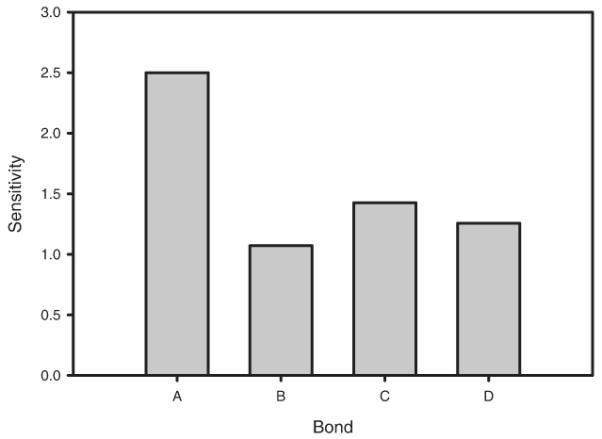
Average sensitivity of normalized RMSD to parameter perturbations for each forward rate constant.

3.3. Inferred Assembly Mechanisms of HPV in Vitro

One of the central goals of fitting computational models to specific viruses is to use simulations to infer experimentally unobservable features of their assembly mechanisms. We therefore wish to determine what the best-fit parameter set suggests to us about assembly mechanisms for the HPV in vitro assembly system. We can infer features of likely assembly pathways by monitoring the production of small intermediates as a function of time. For example, hierarchical assembly mechanisms, in which assembly proceeds by forming oligomers that themselves accrete into complete capsids, can be detected by an early transition of the bulk of the mass fraction of a simulation into the corresponding oligomer [12, 13]. For example, the parameter fits from Section 3.1 inferred that type A (pentameric-hexameric) binding interactions are stronger than any of the hexameric-hexameric interactions; this observation suggests the hypothesis that HPV could use a hierarchical assembly mechanism in which pentameric capsomers are quickly surrounded by hexameric capsomers to form a six-capsomer oligomer, twelve of which would then more slowly come together to form a complete capsid. This particular hierarchical model has been previously suggested for HPV based on structural studies of purified LP1 assembly products [36]. If the hypothesis is true, then we would expect a quick transition of most of the mass fraction of the simulation into hexamers of capsomers, as well as a depletion of species that do not contain multiples of six capsomers. Monitoring intermediate mass fractions also provides a way to test for nucleation-limited assembly, which should show a characteristic pattern of depletion of intermediates of size equal to or greater than the nucleus size.

Figure 8 shows mass fractions versus time for a collection of small intermediates that could potentially serve as nuclei or intermediates for a hierarchical assembly simulation. No small intermediate occupies more than a small fraction of the total mass at any point in the assembly reaction, suggesting that the assembly does not proceed by a hierarchical mechanism. Note that because we model assembly from capsomers, not coat monomers, our model implicitly does encode a hierarchical mechanism involving rapid assembly of capsomers followed by accretion of capsomers into capsids. The data is not, however, consistent with any higher-order hierarchical assembly mechanism involving oligomers of capsomers, such as the hexamer-of-capsomers intermediate hypothesized in the preceding paragraph. More surprisingly, the intermediate data is also inconsistent with nucleation-limited assembly. While the mass fractions tend to decrease with increasing intermediate size, there is only a small change in mass fractions between successive sizes. The mechanism thus appears more consistent with an equilibrium model similar to that proposed by Zlotnick et al. [3, 8, 11] in the absence of an explicit nucleation step. In particular, the data appears to fit a mechanism of assembly by successive accumulation of individual capsomers with no defined slow nucleation step.

Figure 8.

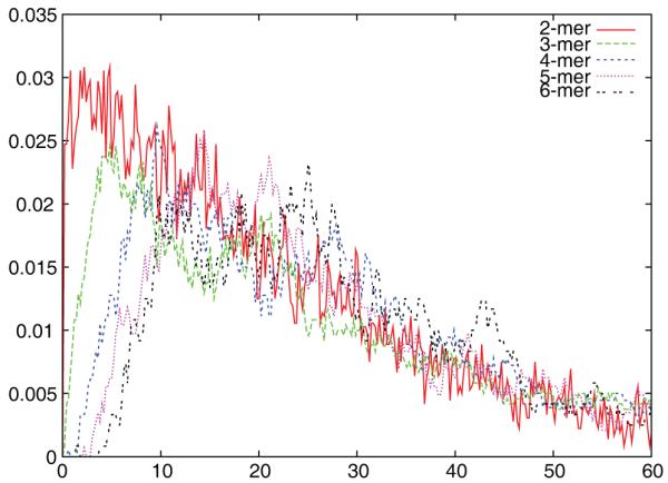
Mass fractions of small intermediates as functions of time for a simulation trajectory using the best-fit HPV rate constants at 145 μg/ml

One important question is whether this behavior would be expected to change under reasonable deviations in the parameters of the system. While the sensitivity studies suggest the overall assembly progress is not greatly affected by small parameter changes, that would not preclude potentially large changes in the assembly mechanisms in response to more dramatic changes in assembly conditions. Earlier theoretical studies had suggested that pathway usage can be highly sensitive to changes in assembly conditions in some regions of the parameter space [13]. Of particular interest is whether changes between the in vitro assembly conditions and in vivo conditions could be sufficient to produce significant overall changes in pathway usage. To explore this question, we examined the intermediate usage in simulations for varying concentrations of initial capsomers. We looked at four specific concentrations: 100 μg/ml, 200 μg/ml, 500 μg/ml, and 1,000 μg/ml. These concentrations were chosen to span a range from a typical low-concentration in vitro assembly condition to a more plausible total concentration feasible in vivo. Figure 9 shows the results. Each concentration shows a similar profile of intermediate mass fractions to that observed for 145 μg/ml. In each case, mass fractions drop slightly with each increasing oligomer size. This observation suggests that the proposed model of assembly by accretion of individual capsomers without a defined nucleation step describes assembly of this system across the range of concentrations examined.

Figure 9.

Mass fractions of small intermediates as functions of time for varying initial capsomer concentrations. Each figure shows mass fraction versus time of monomer, dimer, trimer, tetramer, pentamer, and hexamer oligomers for the best-fit parameters at a distinct concentration: (a) 100 μg/ml. (b) 300 μg/ml. (c) 500 μg/ml. (d) 1000 μg/ml.

4. Conclusions and outlook

We have developed a general method for fitting rate parameters of stochastic models of capsid assembly to experimental measures of assembly progress. The approach combines quasi-gradient-descent and response surface methods in order to deal with the particular challenges of learning rate parameters from capsid assembly simulations, particularly the high computational cost of evaluating the objective function and the stochastic noise inherent to the simulation approach. We further demonstrated the method by fitting a coarse-grained model of HPV assembly to light scattering data from an in vitro HPV assembly system. The method is successful in finding parameters that show generally close fit to the observed experimental data while yielding physically plausible rates and free energies for coat-coat binding. Further analysis shows sufficient sensitivity of the model to variability in each parameter to suggest that the parameters are at least locally optimal for the data to within a small (< 10%) tolerance. This work represents a first step in transitioning the study of quantitative capsid assembly systems from generic phenomenological models of assembly to models of specific viruses. It further provides a general demonstration of how simulation-assisted parameter fitting can be used to learn physical parameters that are not directly experimentally observable for complex biological systems.

The inferred assembly mechanisms for the HPV system are generally consistent with Casini et al.’s own analysis of their data, although with some notable differences in interpretation. We conclude that the first step of assembly is formation of a dimer of capsomers, consistent with Casini et al.’s estimation of a dimeric nucleus size. Likewise, we find that assembly proceeds by accretion of individual capsomers, consistent with Casini et al.’s finding that elongation is a second-order reaction. Our analysis differs from that of Casini et al.’s, however, in concluding that the rate of formation of the initial dimer is comparable to the rate of subsequent elongation steps; we thus suggest that the data is not consistent with a nucleation-limited assembly process, which would require that elongation is much faster than nucleation. We further conclude that this behavior is robust to a broad range of feasible concentrations of the system. This conclusion is unexpected given the observation of nucleation-limited behavior in other in vitro capsid assembly systems [16, 29] and the conclusion of many theoretical studies that nucleation-limited growth is necessary to achieve high yield of fully assembled particles [5, 7–9, 16, 19]. Indeed, our simulations show many incompletely assembled capsids at pseudo-equilibrium, a kinetically trapped state repeatedly observed in simulations when elongation rates are not substantially higher than nucleation rates.

There are several ways one might explain the discrepancy between the expectation of nucleation-limited behavior and the conclusion that the fit parameters do not show such behavior. One possibility is that the method has not fit the true parameters of the system and that a different set of parameters will fit the data at least as well and exhibit nucleation-limited growth. The method used is a local optimization strategy and it is possible that other local optima, possibly exhibiting different assembly mechanisms, could lie elsewhere in the parameter space. This possibility seems unlikely given the appearance of the initial parameter space search (Figure 3), which showed a relatively smooth potential space with a single evident basin of good fit. A related possibility is that the basic coarse-grained model used here is missing some important feature of the real assembly process and cannot match the actual assembly process for any parameter values. While the fit to the experimental data is generally good, there are differences (e.g., the different appearance of the curves in the lag phase) that could suggest some significant discrepancy between the true and inferred assembly mechanisms. For example, our model does not permit any non-native binding interactions during the assembly process, potentially excluding some off-pathway reactions that could influence the nucleation kinetics. It cannot be ruled out that some other model might allow for a very different assembly mechanism but only a slightly different light scattering profile. Our analysis also suggests that fitting to a better model of the output of the measurement apparatus, as opposed to an idealized physical model of light scattering data, may yield improved fits.

One appealing hypothesis is that our method has in fact correctly fit a low yield, non-nucleation limited mechanism to the available in vitro data but that the virus itself uses a different assembly mechanism in vivo. Just as the model may lack some key feature that causes it to assembly in a different way than the real system, so too is it possible that the in vitro system lacks some key feature that causes it to assemble by a different, and perhaps less efficient, mechanism than it would in vivo. It is difficult to speculate on how the assembly mechanisms might differ between in vitro or in vivo assembly because so many features of the in vivo environment are lacking in a purified in vitro assembly system. One key distinction is the lack of the L2 protein, which is not required for assembly of L1 into capsids but co-assembles with L1 in vivo and may affect its nucleation mechanism [37]. Another intriguing difference that may explain a discrepancy is the role of chaperone proteins, which are known to be tightly associated with LP1 capsomers in vivo prior to their assembly but are lacking from the in vitro system [38]. One can speculate that release of these chaperones could act much like a conformational switch in Caspar’s autostery model [39] to slow production of the initial dimer relative to the elongation reactions and prevent kinetic trapping. It is also possible that the system is indeed not nucleation limited in vitro or in vivo and that some unanticipated extra mechanism, such as kinetic proofreading to clear trapped intermediates, ensures high yields in vivo.

There are several avenues by which the present work can be advanced. One key step will be applying the method to other capsid assembly systems in order to verify that one can indeed infer distinct assembly mechanisms in different systems. Light scattering data of various kinds has been gathered for several in vitro systems, including phage P22 [29], hepatitis B virus [16], cowpea chlorotic mottle virus [40], and phage ϕ8 [41], providing a range of systems to which one might fit parameters. In addition, there may be much to be gained from fitting richer data sources than a single static light scattering trajectory as was used in the present work. There is likely also considerable room for improvement in the fitting algorithm itself, including developing better methods to speed the local optimization process and better strategies for approximating a global optimization. Finally, the problem of distinguishing in vitro from in vivo mechanisms raises numerous questions, both experimental and theoretical. From a computational perspective, it will be necessary to develop better models of assembly in vivo and how it differs in general from in vitro. From an experimental perspective, progress will depend on new methods for gathering quantitative data on assembly in vivo. One key hope of this work is that simulation-assisted parameter fitting will provide a way for experimentalists to broaden the range of techniques and data sources available to them by making it possible to learn a great deal about the assembly process from experimental measures that might otherwise be dismissed as uninformative.

References

- [1].Whitesides GM, Mathias JP, Seto CT. Molecular self-assembly and nanochemistry: a chemical strategy for the synthesis of nanostructures. Science. 1991;254(5036):1312–1319. doi: 10.1126/science.1962191. [DOI] [PubMed] [Google Scholar]
- [2].Whitesides GM, Grzybowski B. Self-Assembly at all scales. Science. 2002;295(5564):2418–2421. doi: 10.1126/science.1070821. [DOI] [PubMed] [Google Scholar]
- [3].Zlotnick A. To build a virus capsid: An equilibrium model of the self assembly of polyhedral protein complexes. J. Mol. Biol. 1994;241:59–67. doi: 10.1006/jmbi.1994.1473. [DOI] [PubMed] [Google Scholar]
- [4].Berger B, Shor PW, Tucker-Kellogg L, King J. Local rule-based theory of virus shell assembly. Proc. Natl. Acad. Sci. USA. 1994;91(16):7732–7736. doi: 10.1073/pnas.91.16.7732. [DOI] [PMC free article] [PubMed] [Google Scholar]
- [5].Schwartz R, Shor PW, Prevelige PE, Berger B. Local rules simulation of the kinetics of virus capsid Self-Assembly. Biophys. J. 1998;75(6):2626–2636. doi: 10.1016/S0006-3495(98)77708-2. [DOI] [PMC free article] [PubMed] [Google Scholar]
- [6].Rapaport D, Johnson J, Skolnick J. Supramolecular self-assembly: molecular dynamics modeling of polyhedral shell formation. Comp. Phys. Comm. 1999;122:231–235. [Google Scholar]
- [7].Hagan MF, Chandler D. Dynamic pathways for viral capsid assembly. Biophys. J. 2006;91:42–54. doi: 10.1529/biophysj.105.076851. [DOI] [PMC free article] [PubMed] [Google Scholar]
- [8].Zandi R, van der Schoot P, Reguera D, Kegel W, Reiss H. Classical nucleation theory of virus capsids. Biophys. J. 2006;90:1939–1948. doi: 10.1529/biophysj.105.072975. [DOI] [PMC free article] [PubMed] [Google Scholar]
- [9].Nguyen HD, Reddy VS, Brooks CL. Deciphering the kinetic mechanism of spontaneous self-assembly of icosahedral capsids. Nano Letters. 2007;7(2):338–344. doi: 10.1021/nl062449h. [DOI] [PubMed] [Google Scholar]
- [10].Zhang T, Schwartz R. Simulation study of the contribution of Oligomer/Oligomer binding to capsid assembly kinetics. Biophys. J. 2006;90(1):57–64. doi: 10.1529/biophysj.105.072207. [DOI] [PMC free article] [PubMed] [Google Scholar]
- [11].Keef T, Micheletti C, Twarock R. Master equation approach to the assembly of viral capsids. J. Theoret. Biol. 2006;242(3):713–721. doi: 10.1016/j.jtbi.2006.04.023. PMID: 16782135. [DOI] [PubMed] [Google Scholar]
- [12].Misra M, Lees D, Zhang T, Schwartz R. Pathway complexity of model virus capsid assembly systems. Comp. Meth. Math. Medicine. 2008;9:277–293. [Google Scholar]
- [13].Sweeney B, Zhang T, Schwartz R. Exploring the parameter space of complex Self-Assembly through virus capsid models. Biophys. J. 2008;94(3):772–783. doi: 10.1529/biophysj.107.107284. [DOI] [PMC free article] [PubMed] [Google Scholar]
- [14].Ceres P, Zlotnick A. Weak protein-protein interactions are sufficient to drive assembly of hepatitis B virus capsids. Biochemistry. 2002;41:11525–11531. doi: 10.1021/bi0261645. [DOI] [PubMed] [Google Scholar]
- [15].Parent KN, Zlotnick A, Teschke CM. Qunatitative analysis of multi-component spherical virus assembly: scaffolding protein contributes to the global stability of phage P22 procapsids. J. Mol. Biol. 2006;359:1097–1106. doi: 10.1016/j.jmb.2006.03.068. [DOI] [PubMed] [Google Scholar]
- [16].Zlotnick A, Johnson JM, Wingfield PW, Stahl SJ, Endres D. A theoretical model successfully identifies features of hepatitis b virus capsid assembly. Biochemistry. 1999;38(44):14644–14652. doi: 10.1021/bi991611a. [DOI] [PubMed] [Google Scholar]
- [17].Reddy VS, Giesing HA, Morton RT, Kumar A, Post CB, Brooks CL, Johnson JE. Energetics of quasiequivalence: computational analysis of protein-protein interactions in icosahedral viruses. Biophys. J. 1998;74:546–558. doi: 10.1016/S0006-3495(98)77813-0. [DOI] [PMC free article] [PubMed] [Google Scholar]
- [18].Hemberg M, Yaliraki SN, Barahona M. Stochastic kinetics of viral capsid assembly based on detailed protein structures. Biophys. J. 2006;90(9):3029–3042. doi: 10.1529/biophysj.105.076737. [DOI] [PMC free article] [PubMed] [Google Scholar]
- [19].Endres D, Zlotnick A. Model-based analysis of assembly kinetics for virus capsids or other spherical polymers. Biophys. J. 2002;83:1217–1230. doi: 10.1016/S0006-3495(02)75245-4. [DOI] [PMC free article] [PubMed] [Google Scholar]
- [20].Johnston IG, Louis AA, Doye JPK. Modelling the self-assembly of virus capsids. J. Phys.: Condens. Matter. 2010;22:104101. doi: 10.1088/0953-8984/22/10/104101. [DOI] [PubMed] [Google Scholar]
- [21].Zhang T, Rohlfs R, Schwartz R. Implementation of a discrete event simulator for biological self-assembly systems. Proceedings of the 37th Winter Simulation Conference; Orlando, Florida: 2005. pp. 2223–2231. Winter Simulation Conference. [Google Scholar]
- [22].Wales DJ. The energy landscape as a unifying theme in molecular science. Phil. Trans. R. Soc. A. 2005;363:357–377. doi: 10.1098/rsta.2004.1497. [DOI] [PubMed] [Google Scholar]
- [23].Azadivar F. Simulation optimization methodologies. Proceedings of the 31st Winter Simulation Conference: Simulation—a bridge to the future - Volume 1; Phoenix, Arizona, United States: ACM; 1999. pp. 93–100. [Google Scholar]
- [24].Carson Y, Maria A. Simulation optimization: methods and applications. Proceedings of the 29th Winter Simulation Conference; Atlanta, Georgia, United States: IEEE Computer Society; 1997. pp. 118–126. [Google Scholar]
- [25].Fu M. Optimization via simulation: A review. Annals of Operations Research. 1994;53(1):199–247. [Google Scholar]
- [26].Glynn PW. Optimization of stochastic systems. Proceedings of the 18th Winter Simulation Conference; Washington, D.C., United States: ACM; 1986. pp. 52–59. [Google Scholar]
- [27].Glynn PW. Optimization of stochastic systems via simulation. Proceedings of the 21st Winter Simulation Conference; Washington, D.C., United States: ACM; 1989. pp. 90–105. [Google Scholar]
- [28].Azadivar F, Talavage J. Optimization of stochastic simulation models. Mathematics and Computers in Simulation. 1980;22(3):231–241. [Google Scholar]
- [29].Prevelige PE, Thomas D, King J. Nucleation and growth phases in the polymerization of coat and scaffolding subnits into icosahedral procapsid shells. Biophys. J. 1993;64:824–835. doi: 10.1016/S0006-3495(93)81443-7. [DOI] [PMC free article] [PubMed] [Google Scholar]
- [30].Casini GL, Graham D, Heine D, Garcea RL, Wu DT. In vitro papillomavirus capsid assembly analyzed by light scattering. Virology. 2004;325(2):320–327. doi: 10.1016/j.virol.2004.04.034. [DOI] [PubMed] [Google Scholar]
- [31].Levenberg KA. A mehtod for the solution of certain problems in least squares. Quart. Appl. Math. 1944;2:164–168. [Google Scholar]
- [32].Marquardt D. An algorithm for the least-squares estimation of non-linear parameters. SIAM J. Appl. Math. 1963;11:431–441. [Google Scholar]
- [33].Gillespie DT. A general method for numerically simulating the stochastic time evolution of coupled chemical reactions. J. Comp. Phys. 1976;22(4):403–434. [Google Scholar]
- [34].Li M, Cripe TP, Estes PA, Lyon MK, Rose RC, Garcea RL. Expression of the human papillomavirus type-11 L1 capsid protein in escherichia coli: characterization of protein domains involved in dna-binding and capsid assembly. J. Virol. 1997;71:2988–2995. doi: 10.1128/jvi.71.4.2988-2995.1997. [DOI] [PMC free article] [PubMed] [Google Scholar]
- [35].Tuma Roman. 2010. Personal communication.
- [36].Chen XS, Casini G, Harrison SC, Garcea RL. Papillomavirus capsid protein expression in escherichia coli: purification and assembly of HPV11 and HPV16 L1. J. Mol. Biol. 2001;307:173–182. doi: 10.1006/jmbi.2000.4464. [DOI] [PubMed] [Google Scholar]
- [37].Conway MJ, Meyers C. Replication and assembly of human papillomaviruses. J. Dental Res. 2009;88(4):307–317. doi: 10.1177/0022034509333446. [DOI] [PMC free article] [PubMed] [Google Scholar]
- [38].Garcea RL. 2008. Personal communication.
- [39].Caspar DLD. Movement and self-control in protein assemblies: quasi-equivalence revisited. Biophys. J. 1980;32 doi: 10.1016/S0006-3495(80)84929-0. [DOI] [PMC free article] [PubMed] [Google Scholar]
- [40].Zlotnick A, Aldrich R, Johnson JM, Ceres P, Young MJ. Mechanism of capsid assembly for an icosahedral plant virus. Virology. 2000;277:450–456. doi: 10.1006/viro.2000.0619. [DOI] [PubMed] [Google Scholar]
- [41].Kainov DE, Butcher SJ, Bamford DH, Tuma R. Conserved intermediates on the assembly pathway of double-stranded RNA bacteriophages. J. Mol. Biol. 2003;328:791–804. doi: 10.1016/s0022-2836(03)00322-x. [DOI] [PubMed] [Google Scholar]