Functional Connectivity: Shrinkage Estimation and Randomization Test

Abstract

We develop new statistical methods for estimating functional connectivity between components of a multivariate time series and for testing differences in functional connectivity across experimental conditions. Here, we characterize functional connectivity by partial coherence, which identifies the frequency band (or bands) that drives the direct linear association between any pair of components of a multivariate time series after removing the linear effects of the other components. Partial coherence can be efficiently estimated using the inverse of the spectral density matrix. However, when the number of components is large and the components of the multivariate time series are highly correlated, the spectral density matrix estimate may be numerically unstable and consequently gives partial coherence estimates that are highly variable. To address the problem of numerical instability, we propose a shrinkage-based estimator which is a weighted average of a smoothed periodogram estimator and a scaled identity matrix with frequency-specific weight computed objectively so that the resulting shrinkage estimator minimizes the mean-squared error criterion. Compared to typical smoothing-based estimators, the shrinkage estimator is more computationally stable and gives a lower mean squared error. In addition, we develop a randomization method for testing differences in functional connectivity networks between experimental conditions. Finally, we report results from numerical experiments and analyze an EEG data set recorded during a visually-guided hand movement task.

Introduction

Functional connectivity is defined in Friston et al. (1993) as the “temporal correlation of spatially remote neurophysiogical events.” Neurophysiological signals simultaneously obtained from different regions of the brain give rise to data in the form of a multivariate time series. Here, we characterize functional connectivity via partial coherence between each pair of signals in a multivariate time series and develop a novel method for modeling and estimating the cross-dependence structure.

Frequency domain metrics have been used successfully for investigating the dependency structure of multivariate neurophysiological signals (Timmer et al., 2000; Mirski et al., 2003; Sun et al., 2004; Salvador et al., 2005). The most common frequency domain cross-dependency metric is coherence, which is a time-invariant metric of pair-wise linear association. Coherence is the frequency domain analog of cross-correlation (Brillinger, 2001) and is derived from the spectral density matrix. In a P-channel multivariate time series, the spectral density matrix is a P ×P semipositive Hermitian matrix which is approximately equal to the covariance matrix of the P-dimensional vector of Fourier coefficients computed for each frequency. However, in multivariate time series, simply using cross-correlation or coherence between the components can lead to misleading conclusions on the cross-dependence structure of the signals (Kus et al., 2004). Neither can distinguish between a pair of components that are directly linked versus a pair that is indirectly linked through a third component. Thus, to have a better understanding on how two components directly interact with each other, it is necessary to remove the effects of the other components.

In the time domain, a metric for direct linear association is partial cross-correlation. In fMRI studies, partial cross-correlation has been used for removing the temporal effects of experimental designs (McIntosh et al., 1994) and for removing the effects of other brain signals of interest (Marrelec et al., 2006). The frequency domain analog of partial cross-correlation is partial coherence. It has been successfully implemented in analyzing scalp EEG (Timmer et al., 2000), intracortical EEG (Mirski et al., 2003), and fMRI (Sun et al., 2004, Zhou et al, 2009). As we will describe in further detail, an efficient approach to estimating partial coherence involves inversion of the spectral density matrix. This approach requires estimates of the spectral density matrix to be numerically stable because otherwise, even small perturbations in the estimates of the spectral density matrix will result in large changes in the entries of its inverse, consequently giving highly variable partial coherence estimates.

We develop a novel shrinkage estimation method for estimating functional interconnectivity across brain sites. The shrinkage estimator is a weighted average of a mildly-smoothed periodogram matrix and the scaled identity matrix. The resulting shrinkage estimates have lower condition numbers than the classical smoothed periodogram and hence are more numerically stable. Böhm (2008) developed shrinkage estimation for the spectral density matrix of multivariate time series in a single-trial setting. We extend the shrinkage estimator to handle multiple-trial multivariate time series and, via numerical experiments, demonstrate that it does well in estimating both the spectral density matrix and partial coherence. We also develop a randomization procedure for testing for differences in functional connectivity between experimental conditions. We apply these new methods to an electroencephalogram (EEG) data set acquired from an experiment to study the brain network that mediates voluntary movement.

Methods

Participants and brain recordings

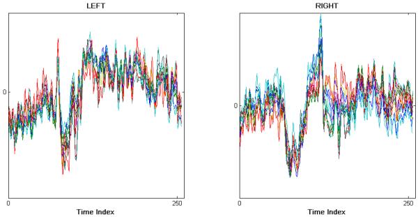
The EEG data reported upon in this paper were selected from a group of 11 healthy, young adults (20-35 yr, mean 25 yr), from whom we recorded potentials from the scalp using a 64-channel EEG system (EMS, Biomed, Korneuburg, Germany). The electrodes were applied to the scalp using conventional methods arrayed in the standard International 10-20 system, two of which served as a ground and a reference, leaving 62 active EEG leads. We recorded the EEG at 512 Hz using a high-pass lter of 0.02 Hz and a low-pass lter of 100 Hz. Participants performed a visually-guided hand movement task. In this task, the comfortably seated volunteers viewed a video monitor, placed about one meter away, and they responded to targets that jumped to the left or right from a central position. A target jump, occurring every 1.5-5 seconds, instructed the participant to displace the lever of a hand-held joystick (Mag Design and Engineering, Sunnyvale, CA) from a central upright position to realign the visual representation of the joystick orientation with the displaced target, either to the right or left of center. Participants received instructions to start and to move quickly and accurately, and to return the joystick to the center position only when the target jumped back to the center of the video monitor. We analyzed EEG signals for 118 leftward and 138 rightward movements from the center position, performed randomly. Figure 1 illustrates time-amplitude plots of the 12 EEG signals obtained from a representative participant during leftward (Figure 1, left) and rightward (Figure 1, right) joystick movements.

Figure 1.

Left: representative 12-channel EEG recorded from one trial for the left condition. Right: representative 12-channel EEG recorded from one trial for the right condition.

From the montage of 64 scalp electrodes, we selected a sub-set of 12 surface leads from five representative participants from which we assessed coherence among the EEG recordings. The electrode sites overlay regions presumed, a priori, to have involvement in neural processes engaged in visual-motor actions (e.g., Marconi et al., 2001; Bédard and Sanes, 2009). Subsequent studies will include assessment of EEG record from all sensors and also entail source analysis. The current work was designed to explore the validity of the partial coherence method as a tool to reveal connectivity across brain sites, particularly those expected to have involvement in the visual-motor task used for this work. Thus, we assessed partial coherence from EEG recorded between the following sensors: FC3, FC5, C3, P3, and O1 over the left hemisphere; FC4, FC6, C4, P4 and O2 over the right hemisphere; and Cz and Oz over the mid-line. The frontal (FC) leads were presumably placed over the prefrontal cortex, regions previously shown to have involvement in premotor processing. The central (C) leads were placed over structures involved in motor performance, while the parietal (P) and occipital (O) leads were placed over structures involved in visual sensation and visual-motor transformations (Marconi et al., 2001).

Partial coherence as a metric for functional connectivity

Partial coherence is a useful metric of dependency because it is highly specific in the sense that it identifies the frequency bands that drive the direct linear association between EEG signals. Using partial coherence does not require one to impose a rigid parametric structure on the hypothesized network and hence is robust to model misspecification. In addition, partial coherence has an appealing interpretation. Ombao and Van Bellegem (2008) showed that coherence and partial coherence are equivalent to the cross-correlation and partial cross-correlation, respectively, between filtered signals. Consider, for instance, a trivariate time series X(t) = [U(t), V (t), Z(t)]’. First, apply a bandpass filter to each component to obtain X_ω(t) = [U_ω(t), V_ω(t), Z_ω(t)]’. Then the coherence between U(t) and V (t) at frequency ω is equivalent to the cross-correlation between the filtered time series U_ω(t) and V_ω(t). However, the linear association at frequency ω between U(t) and V (t) may be confounded by the third component Z(t). So to obtain a measure of direct association between U(t) and V (t), we must remove the effect Z(t). This motivates the use of partial coherence.

In the following discussion, we present two general strategies for estimating partial coherence. We demonstrate that when the number of components is large, a one-step procedure that uses the inverse of the spectral matrix is more mathematically elegant and efficient than the recursive procedure.

A recursive procedure for estimating partial coherence

The following is one approach to estimate partial coherence as described by Brillinger (2001) and further discussed by Medkour et al. (2009). Let f_UV (ω) be the cross-spectra between U(t) and V (t), and similarly define f_UZ(ω) and f_ZV (ω). Let f_ZZ(ω) be the spectral density for Z(t). Then the partial coherence between U(t) and V (t) is given by

$${\rho }_{UV\mid Z}^2\left(\omega \right)=\frac{{\mid {\mathbf{g}}_{UV\mid Z}\left(\omega \right)\mid }^2}{{\mathbf{g}}_{UU\mid Z}\left(\omega \right){\mathbf{g}}_{VV\mid Z}\left(\omega \right)},$$ (1)

where

$${\mathbf{g}}_{ij\mid Z}\left(\omega \right)={\mathbf{f}}_{ij}\left(\omega \right)-{\mathbf{f}}_{iZ}\left(\omega \right){\mathbf{f}}_{ZZ}^{-1}\left(\omega \right){\mathbf{f}}_{Zj}\left(\omega \right).$$ (2)

Equation (2) can be interpreted as the autospectra or cross-spectra after removing the linear effects of Z(t), e.g., g_UU∣Z(ω) is the autospectra of U(t) after the linear effects of Z(t) have been removed. Note how Equation (1) is analogous to the definition of the squared partial cross-correlation.

Now suppose that we have a 4-variate time series [U(t), V (t), Z₁(t),Z₂(t)]’, and that we wish to obtain the partial coherence between U(t) and V (t) after removing the linear effects of Z₁(t) and Z₂(t). The procedure for computing partial coherence becomes recursive. First, let

$${\mathbf{f}}_{ij\mid Z_1}\left(\omega \right)={\mathbf{f}}_{ij}\left(\omega \right)-{\mathbf{f}}_{i{Z}_1}\left(\omega \right){\mathbf{f}}_{Z_1{Z}_1}^{-1}\left(\omega \right){\mathbf{f}}_{Z_{1}j}\left(\omega \right),$$ (3)

and define

$${\mathbf{g}}_{ij\mid Z_1{Z}_2}\left(\omega \right)={\mathbf{f}}_{ij\mid Z_1}\left(\omega \right)-{\mathbf{f}}_{i{Z}_2\mid Z_1}\left(\omega \right){\mathbf{f}}_{Z_2{Z}_2\mid Z_1}^{-1}\left(\omega \right){\mathbf{f}}_{Z_{2}j\mid Z_1}\left(\omega \right).$$ (4)

Then the partial coherence between U(t) and V (t) is given by

$${\rho }_{UV\mid Z_1{Z}_2}^2\left(\omega \right)=\frac{{\mid {\mathbf{g}}_{UV\mid Z_1{Z}_2}\left(\omega \right)\mid }^2}{{\mathbf{g}}_{UU\mid Z_1{Z}_2}\left(\omega \right){\mathbf{g}}_{VV\mid Z_1{Z}_2}\left(\omega \right)},$$ (5)

Equation (3) removes the linear effect of Z₁(t) and can be computed using the appropriate entries from the spectral density matrix. The resulting values can then be used in Equation (4), which removes the linear effect of Z₂(t). Finally, the partial coherence between U(t) and V (t) can be calculated using Equation (5). This recursive procedure is repeated again to obtain the partial coherence between all pairs of signals: ${\rho }_{U{Z}_1\mid V{Z}_2}^2\left(\omega \right)$, ${\rho }_{U{Z}_2\mid V{Z}_1}^2\left(\omega \right)$, ${\rho }_{V{Z}_1\mid U{Z}_2}^2\left(\omega \right)$, ${\rho }_{V{Z}_2\mid U{Z}_1}^2\left(\omega \right)$, and ${\rho }_{Z_1{Z}_2\mid UV}^2\left(\omega \right)$.

We can see that as the number of components in our signals increase, we must proceed through many more layers of this recursive procedure, where at each step we remove the linear effects of one of the components. Moreover, with this procedure, the estimated entries of the spectral density matrix are simply plugged into the inital step [e.g., for each of f_UU∣Z1(ω), f_{V V∣Z1} (ω), and f_{UV ∣Z1} (ω) in Equation (3)] before nally obtaining an estimate of the partial coherence for each pair of components. As a result, the variability in the estimation of the entries of the spectral density matrix will propagate and accumulate and will certainly affect the estimate of the partial coherence. Thus, this procedure is not computationally nor statistically efficient for obtaining all pair-wise partial coherence values for all frequencies.

A one-step procedure for estimating partial coherence

An equivalent and substantially more efficient way of obtaining all pairwise partial coherence for all frequencies is via the inverse of the spectral density matrix. This approach is described by Dahlhaus (2000) and has been used by Eichler et al. (2003) for neural spike trains, Medkour et al. (2009) for EEG, and Salvador et al. (2005) for fMRI. We outline a systematic approach given by Dahlhaus (2000).

Let X(t) = [X₁(t), …, X_P (t)]’ be a stationary P-channel multivariate time series with mean $\mathbb{E}\mathbf{X}\left(t\right)=0$ and spectral density matrix f(ω). The diagonal elements of f(ω), denoted f_pp(ω), p = 1, …, P, are the auto-spectra of the P channels and the off-diagonal elements, denoted f_pq(ω), are the cross-spectra between channels X_p(t) and X_q(t). Define the matrix g(ω) = f⁻¹(ω) and denote the diagonal elements as g_pp(ω). Let h(ω) be a diagonal matrix whose elements are ${\mathbf{g}}_{pp}^{-1∕2}\left(\omega \right)$. Define the matrix Γ(ω) to be

$$\Gamma \left(\omega \right)=-\mathbf{h}\left(\omega \right)\mathbf{g}\left(\omega \right)\mathbf{h}\left(\omega \right).$$ (6)

Then, the partial coherence between the p and q-th channels is the modulus squared of the (p, q)-th element of Γ(ω), i.e.,

$${\rho }_{pq}^2\left(\omega \right)={\mid {\Gamma }_{pq}\left(\omega \right)\mid }^2.$$ (7)

Thus, all pairwise partial coherence estimates can be computed simultaneously using the inverse of the spectral density matrix.

Numerical instability of the estimated spectral density matrix

To use the above estimate of partial coherence, we first need to estimate the spectral density matrix. Define d(ω) to be the P-dimensional vector of Fourier coefficients of each component where the p-th component is d_p(ω) = ∑_t X_p(t) exp(−iωt). Let $\mathbf{I}\left(\omega \right)=\frac{1}{T}\mathbf{d}\left(\omega \right){\mathbf{d}}^{\ast }\left(\omega \right)$ be the raw periodogram matrix. The classical nonparametric estimator for spectral matrix is the smoothed periodogram matrix f̃(ω) = smooth_{λ in N(ω)}I(λ) where N(ω) is a small neighborhood (band) around ω. Under regularity conditions, the resulting estimator is asymptotically mean squared consistent, but it can have a poor condition number (much larger than 1) or even be non-invertible if the number of discrete frequencies in N(ω) is not larger than the dimension P. The condition number of the estimated spectral matrix is the ratio of the largest eigenvalue to the smallest eigenvalue. It quantifies the effect of a small perturbation in the data on the inverse of the spectral density matrix, so that well-conditioned spectral density matrices have condition numbers that are close to 1. It is possible that the entries in the inverse of this matrix, as needed for partial coherence estimation, are numerically unstable.

To obtain numerically stable estimates, it is necessary for the estimate of the spectral density matrix to be well-conditioned. However, estimators based on the smoothed periodogram have maximum eigenvalue that tend to overestimate the true maximum eigenvalue and minimum eigenvalues that tend to underestimate the true minimum eigenvalue. Thus, the condition number of the estimators is biased upwards, i.e., is relatively more ill-conditioned (Böhm and von Sachs, 2009). One approach to getting well-conditioned estimates of the spectral density matrix is by shrinkage towards a scaled identity matrix.

Other estimators of the spectral density matrix include the Welch periodogram estimator, as utilized by Sun et al. (2004) for fMRI analysis, and the multitaper, as described in Thomson (1982) and Walden (2000) and used by Medkour et al. (2009) for EEG analysis. The Welch periodogram estimator yields an estimator with low variance but can have poor frequency resolution because it computes periodograms from smaller time blocks (thus with fewer observations per time block). The multitaper procedure, on the other hand, can yield both low bias and variance by picking the proper number of tapers. However, neither the Welch nor multitaper methods guarantee that the resulting estimates are simultaneously well-conditioned and localized in frequency. The shrinkage estimator is obtained as the minimizer of the total mean squared error criterion (sum of the variance and the square of the bias over all entries of the spectral density matrix). The shrinkage estimator does not split the time series into smaller time blocks so it has better frequency resolution than the Welch periodogram and, as we will later describe, the shrinkage weight for the shrinkage estimator is constructed so that the total mean squared error is minimized. Thus, its performance is comparable to the multitaper. A desirable property of the shrinkage estimator is that it has a condition number that has been shrunk closer to 1 and hence, it is relatively more well-conditioned than either the Welch or multitaper estimators.

Two potential problems that affect the stability of the spectral density matrix are high-degrees of multicollinearity in the data and side-lobe leakage (Medkour et al., 2009). The latter problem can be addressed by passing the multivariate time series through a linear lter. Böhm (2008) showed results of a simulation in which the estimation of the spectral density matrix via shrinkage improves further if the data are passed through a linear lter. The shrinkage estimator we propose will address the former problem.

Theoretical motivation for the shrinkage estimator

Shrinkage estimators in general are known to have desirable properties. First, shrinkage estimators have lower mean squared error than the classical smoothed periodogram matrix. We refer the reader to Böhm (2008) and Böhm and von Sachs (2009) for technical details. Moreover, shrinkage estimators are easy to implement and give results that are numerically stable. The shrinkage estimator is guaranteed to have a lower condition number than the smoothed periodogram. Thus, the estimate of the inverse of the spectral density matrix and, consequently, the estimates of partial coherence are expected to be more numerically stable.

Medkour et al. (2009) describes a similar idea for regularizing the spectral density matrix for EEG signals estimated via the multitaper procedure. Their approach is to upweight the diagonal elements of the estimated spectral density to increase the minimum eigenvalue, and hence, improve the condition number. The philosophy behind their approach is to upweight the diagonal elements enough to dampen the effects of side-lobe leakage on the estimation of the spectral density matrix. In contrast, the shrinkage approach we will describe is a weighted average of an initial estimator f̃(ω) and an energy-preserving estimator μ(ω)1. This is similar to downweighting the initial estimator – in particular, its diagonal elements – and then adding positive scalars to the diagonal elements of the downweighted initial estimator. While both approaches respond to the need for having well-conditioned estimates, our proposed shrinkage procedure data-adaptively selects the weights that gives the estimator having the smallest mean-squared error.

Estimating and testing for differences in functional connectivity

First, we propose the shrinkage estimator that yields a relatively more numerically stable estimate of partial coherence. Second, to test for differences in functional connectivity, we describe a simple randomization procedure. Our estimation and testing methods both consider the problem of numerical instability throughout the statistical analysis of functional connectivity.

Shrinkage estimation for partial coherence

To obtain a stable estimate of partial coherence, we first need to provide a numerically stable estimate of the spectral density matrix f(ω). The shrinkage estimator, denoted f̂(ω), is a weighted average of the mildly-smoothed periodogram f̃(ω) and the scaled identity matrix μ(ω)1:

$$\widehat{\mathbf{f}}\left(\omega \right)=W\left(\omega \right)\mu \left(\omega \right)1+(1-W(\omega \left)\right)\tilde{\mathbf{f}}\left(\omega \right),$$ (8)

where W(ω) is the shrinkage weight. The scale μ(ω) is the mean power in the multivariate time series so that the shrinkage estimator will preserve the energy in the sample. The shrinkage weight W(ω) is constructed so that the mean squared error is minimized. The formula for the weight W(ω) is reported in the Appendix.

Böhm (2008) derived the analytical form of the shrinkage weight and showed that it is proportional to the total mean squared error of the smoothed periodogram. If the smoothed periodogram has small error, then most of the weight will be shifted toward f̃(ω). Böhm (2008) also gives a procedure for estimating the weight, and shows that the resulting shrinkage estimator is mean squared consistent. However, the method in Böhm is based on only having a single multivariate time series. We adapt the procedure given by Böhm (2008) to our situation where we have several multivariate time series recordings (e.g., multichannel EEGs from several trials).

We now describe how to construct the shrinkage estimator. First define the n-th trial multivariate time series to be X_n(t) = [X_n1(t), …, X_nP (t)]’, where n = 1, …, N and t = 1, …, T. For each trial X_n(t), we can obtain a trial-specific estimator f_n(ω) for the spectral density matrix by smoothing the raw periodogram matrix for that particular trial. If we assume that the underlying process is stationary, then a reasonable estimator for the spectral density matrix is the average of these trial-specific estimators, i.e.,

$$\tilde{\mathbf{f}}\left(\omega \right)=N^{-1}\sum _{n=1}^N{\tilde{\mathbf{f}}}_n\left(\omega \right).$$ (9)

We compute the mean power

$$\mu \left(\omega \right)=P^{-1}\sum _{j=1}^P{\tilde{f}}_{jj}\left(\omega \right),$$ (10)

where f̃_jj(ω) denotes the (j, j)-th element of f̃(ω). What remains is to provide an optimal estimate for the shrinkage weight. We motivate and describe the procedure for estimating the weight in the Appendix.

Using the shrinkage estimate f̂(ω) of the spectral density matrix f(ω), we can proceed with estimating partial coherence. Following Equation (6), we obtain an estimator for Γ(ω) as follows. First, we get ĝ(ω) = f̂⁻¹(ω) via (8) and define ĥ(ω) to be a diagonal matrix whose elements are ${\widehat{\mathbf{g}}}_{pp}^{-1∕2}\left(\omega \right)$. The estimator for the matrix Γ(ω) is

$$\widehat{\Gamma }\left(\omega \right)=-\widehat{\mathbf{h}}\left(\omega \right){\widehat{\mathbf{f}}}^{-1}\left(\omega \right)\widehat{\mathbf{h}}\left(\omega \right)$$ (11)

and so the estimated partial coherence between channels p and q is the modulus squared of the (p, q)-th element of $\widehat{\Gamma }\left(\omega \right)$,

$${\widehat{\rho }}_{pq}^2\left(\omega \right)={\mid {\widehat{\Gamma }}_{pq}\left(\omega \right)\mid }^2.$$ (12)

Algorithm for constructing the shrinkage estimator for the spectral density matrix

The following is a step-by-step procedure for constructing the shrinkage estimator.

• Step 1. For each trial, transform the multivariate time series to the frequency domain to obtain the raw periodogram matrix. Average the raw periodogram matrices over the trials.

• Step 2. Smooth each trial-specific periodogram matrix and use Equation (9) to obtain f̃(ω).

• Step 3. Use Equation (10) to estimate the mean power.

• Step 4. Use Equation (17) to estimate the shrinkage weight W(ω). The procedure is given in the Appendix.

• Step 5. Finally, use Equation (8) to construct the shrinkage estimator f̂(ω).

Randomization test for comparing functional connectivity

Once we have used the shrinkage estimator to estimate functional connectivity for each experimental condition, we would like to look for differences in functional connectivity across experimental conditions. Our approach to accomplish this goal is to use a randomization test. The randomization test does not rely on strong assumptions about the data, making it more robust relative to parametric procedures for hypothesis tests, and has been successfully implemented in the analysis of brain signals (e.g., Nichols and Holmes, 2001; Raz et al., 2003).

The randomization procedure proceeds as follows. Under the null hypothesis that functional connectivity does not vary across conditions, we can change condition labels because the condition should not matter as far as functional connectivity is concerned. We create an empirical distribution of differences in connectivity under the null hypothesis of no difference by resampling and then relabeling the data under the assumptions that the signals are stationary and that the multivariate time series from the trials in the experiment are independent.

Let L_n(t) = [L_n1(t), …, L_nP (t)]’ and R_m(t) = [R_m1(t), …, R_mP (t)]’, n = 1, …, N and m = 1, … M denote the observations from n-th and m-th trial from experiment conditions “leftward” and “rightward” movements, respectively. The algorithm of the randomization procedure is as follows:

• Step 1. Draw ${\mathbf{L}}_n^b\left(t\right)$ and ${\mathbf{R}}_m^b\left(t\right)$, n = 1, …, N and m = 1, …, M, each with replacement from the pooled data set {L₁(t), …, L_N(t), R₁(t), …, R_M(t)}. Call this the b-th pseudo-data set.

• Step 2. Use Equation (12) to estimate the partial coherences ${\left\{{\widehat{\rho }}_{L,pq}^{2,\left(b\right)}\right(\omega \left)\right\}}_{pq}$ for ${\left\{{\mathbf{L}}_n^b\right(t\left)\right\}}_{n-1}^N$ and ${\left\{{\widehat{\rho }}_{R,pq}^{2,\left(b\right)}\right(\omega \left)\right\}}_{pq}$ for ${\left\{{\mathbf{R}}_m^b\right(t\left)\right\}}_{m-1}^M$. Compute ${\left\{{\Delta }_{pq}^b\right(\omega \left)\right\}}_{pq}={\left\{{\widehat{\rho }}_{L,pq}^{2,\left(b\right)}\right(\omega )-{\widehat{\rho }}_{R,pq}^{2,\left(b\right)}(\omega \left)\right\}}_{pq}$.

• Step 3. Repeat Step 1 and Step 2 B times to construct an empirical distribution for the differences.

• Step 4. Using the observed data, compute ${\left\{{\Delta }_{pq}\right(\omega \left)\right\}}_{pq}={\left\{{\widehat{\rho }}_{L,pq}^{2,\left(b\right)}\right(\omega )-{\widehat{\rho }}_{R,pq}^{2,\left(b\right)}(\omega \left)\right\}}_{pq}$. Reject the null hypothesis of no difference between conditions in connectivity between the p-th and q-th channels if Δ_pq(ω) is in the upper or lower tails of the empirical distribution.

Results

Numerical experiment

Using synthetic data, we compared the performance of the shrinkage estimator against the standard approaches, namely, the smoothed periodogram as given in Equation (9) and the multitaper with 15 orthogonal tapers. For the smoothed periodogram, we smoothed around a neighborhood of M = 21 discrete frequencies. For the multitaper estimate, we used the multitaper to estimate the spectral density matrix for each trial, and then took the average of these estimates across all trials. We then compared the total mean squared error of the methods.

In our numerical experiment, one synthetic dataset consisted of N = 100 trials, with each trial with P = 15 channel multivariate time series with T = 256 time points. The time series data were generated from a 15-dimensional second-order vector autoregressive process: X(t) = φ₁X(t − 1) + φ₂X(t − 2) + ∈(t). The noise ∈(t) was drawn from a 15-dimensional Gaussian distribution with covariance matrix the identity matrix. The coefficient matrices φ₁ and φ₂ were

$${\Phi }_1=\left(\begin{array}{ccccc}\hfill {\varphi }^{\left(1\right)}\hfill & \hfill 0\hfill & \hfill 0\hfill & \hfill 0\hfill & \hfill 0\hfill \\ \hfill 0\hfill & \hfill {\varphi }^{\left(2\right)}\hfill & \hfill 0\hfill & \hfill 0\hfill & \hfill 0\hfill \\ \hfill 0\hfill & \hfill 0\hfill & \hfill {\varphi }^{\left(1\right)}\hfill & \hfill 0\hfill & \hfill 0\hfill \\ \hfill 0\hfill & \hfill 0\hfill & \hfill 0\hfill & \hfill {\varphi }^{\left(2\right)}\hfill & \hfill 0\hfill \\ \hfill 0\hfill & \hfill 0\hfill & \hfill 0\hfill & \hfill 0\hfill & \hfill {\varphi }^{\left(1\right)}\hfill \end{array}\right),{\Phi }_2=\left(\begin{array}{ccccc}\hfill {\varphi }^{\left(3\right)}\hfill & \hfill 0\hfill & \hfill 0\hfill & \hfill 0\hfill & \hfill 0\hfill \\ \hfill 0\hfill & \hfill {\varphi }^{\left(3\right)}\hfill & \hfill 0\hfill & \hfill 0\hfill & \hfill 0\hfill \\ \hfill 0\hfill & \hfill 0\hfill & \hfill {\varphi }^{\left(3\right)}\hfill & \hfill 0\hfill & \hfill 0\hfill \\ \hfill 0\hfill & \hfill 0\hfill & \hfill 0\hfill & \hfill {\varphi }^{\left(3\right)}\hfill & \hfill 0\hfill \\ \hfill 0\hfill & \hfill 0\hfill & \hfill 0\hfill & \hfill 0\hfill & \hfill {\varphi }^{\left(3\right)}\hfill \end{array}\right),$$

where

$${\varphi }^{\left(1\right)}=\left(\begin{array}{ccc}\hfill .2\hfill & \hfill 0\hfill & \hfill .02\hfill \\ \hfill .02\hfill & \hfill .2\hfill & \hfill 0\hfill \\ \hfill 0\hfill & \hfill .02\hfill & \hfill .2\hfill \end{array}\right),{\varphi }^{\left(2\right)}=\left(\begin{array}{ccc}\hfill 0.5\hfill & \hfill 0\hfill & \hfill 0\hfill \\ \hfill 0\hfill & \hfill -.05\hfill & \hfill 0\hfill \\ \hfill 0\hfill & \hfill 0\hfill & \hfill .05\hfill \end{array}\right),$$

and

$${\varphi }^{\left(3\right)}=\left(\begin{array}{ccc}\hfill 0.5\hfill & \hfill 0\hfill & \hfill 0\hfill \\ \hfill 0\hfill & \hfill -.05\hfill & \hfill 0\hfill \\ \hfill 0\hfill & \hfill 0\hfill & \hfill .05\hfill \end{array}\right).$$

We generated 1500 synthetic data sets. For each data set, we estimated the spectral density matrix and the matrix of partial coherence values ρ²(ω). For each frequency and for each data set, we evaluated the total squared error over all of the entries of the spectral density matrix. We then averaged the total squared error across the data sets to obtain an estimate of the mean squared error. This allowed us to evaluate efficacy of each estimator at each frequency. To summarize the total mean squared error, we used the integrated mean squared error (IMSE) which is the sum (across all frequencies) of the average squared error per synthetic data. We also provided the integrated standard error of the MSE to demonstrate that the shrinkage method gave less variable results.

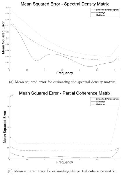
From Figure 2, we see that the shrinkage estimator has smaller mean squared error than the smoothed periodogram over all frequencies, just as we expected. The weight of the shrinkage estimator was picked to minimize mean squared error, and this is illustrated in the standard error of the IMSE in Table 1. Moreover, the standard error demonstrates that the shrinkage method gave less variable results for both the entries of the spectral density matrix and partial coherence. Though the shrinkage estimator is intended to be an estimator for the spectral density matrix, we see large improvements over the smoothed periodogram for estimating partial coherence. Moreover, we also see that the shrinkage estimator can be competitive with the multitaper.

Figure 2.

Mean squared error estimated via Monte Carlo.

Table 1.

Comparison of the three estimators. Reported values are the integrated empirical mean-squared error (IMSE) averaged over 1500 synthetic data sets. Values in parenthesis are the standard deviation of the empirical IMSE.

Estimator	Spectral Density Matrix	Partial Coherence
Smoothed Periodogram	2.1886 (0.2126)	19.856 ×10−4 (4.6415 ×10−4)
Shrinkage	1.0797 (0.0980)	1.6937 ×10−4 (0.5859 ×10−4)
Multitaper	1.5560 (0.1527)	9.3517 ×10−4 (2.3293 ×10−4)

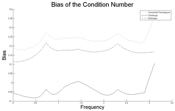
We have so far shown the performance of the shrinkage estimator with respect to mean-squared error. Recall that the goal of the shrinkage estimator is to provide a numerically stable estimate of the spectral density matrix. To illustrate that this is the case, we look at the condition numbers of each of the competing estimators as shown in Figure 3. We note that, as expected, the smoothed periodogram has condition numbers that are biased upwards over all frequencies. The condition numbers for the multitaper are also biased upwards. The shrinkage estimator does not yield unbiased estimates of the condition numbers. Rather, the shrinkage estimator corrects for the upward bias of the smoothed periodogram by shrinking the condition number down.

Figure 3.

Bias of each estimator estimated via Monte Carlo.

Analysis of the EEG Dataset

While the novel shrinkage method is applicable to general multivariate time series, here we applied it to an EEG sensor dataset recorded during rapid, discrete hand movements performed in response to visual cues (see Methods). To illustrate the new method, we compared connectivity occurring during the leftward and rightward experimental conditions.

First, for each condition, and for each pair of channels p, q, we tested the null hypothesis of zero partial coherence over a frequency band of interest. We used Equation (12) to estimate ${\rho }_{pq}^2\left(\omega \right)$ at each frequency, and then take the average over the frequencies in the frequency band of interest to obtain an estimate of partial coherence at that particular frequency band. To obtain a significance threshold for partial coherence, we followed the result given by Eichler (2007). To conservatively control for multiple tests between all possible pairs of regions and within a frequency band, we tested H₀ at level α = 10⁻⁶.

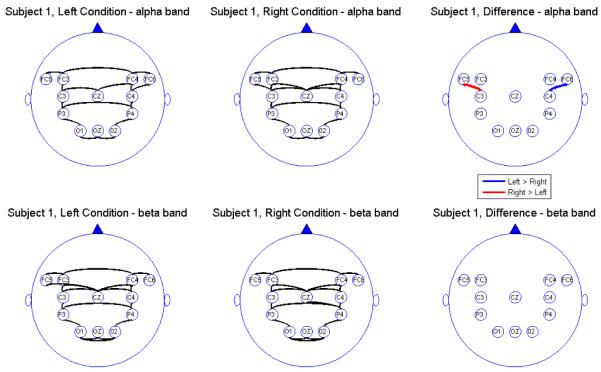
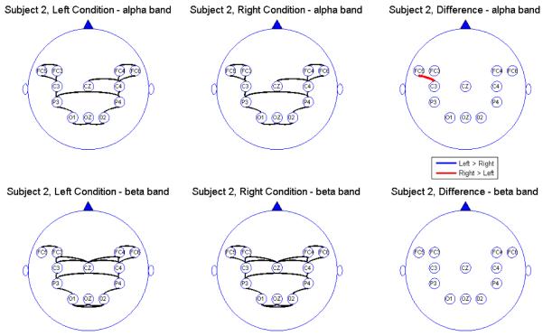
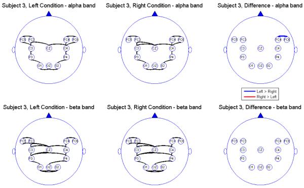
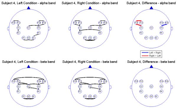
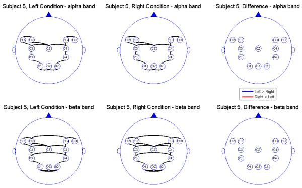
Next, after having obtained the point estimates for partial coherence for each condition, we tested the difference between the two conditions, i.e., we tested the hypothesis H₀ : Δ(ω) = 0 versus H₀ : Δ(ω) ≠ 0, where Δ(ω) is the difference across conditions in partial coherence at a frequency band of interest. We tested H₀ at level α = .05 using B = 5000 bootstrapped samples. In this analysis, we assumed that the EEGs were uncorrelated across trials. We believe that this assumption is reasonable given that there is approximately a 4 second time period between the last observation of a trial and the rst observation of the next trial. Moreover, we computed the cross-correlation values between trials (using the last few time points of one trial and the first few of the next) and noted that the between-trial squared correlation is on the lower quartile (lower tail) of the empirical distribution of the within-trial squared correlation. This suggests that between-trial correlation should not make a very strong impact when performing inference on within-trial connectivity. We then considered only the significant differences between regions p and q conditional on having rejected the hypothesis H₀ : ∣ρ_pq(ω)∣² = 0 for at least one of the conditions. The results across participants were varied but due to the small sample size it was not sensible to perform a group-level analysis. We present results of the single-subject analyses for each of the ve subjects. The connectivity maps and difference maps for each of the subjects are displayed in Figures 4, 5, 6, 7, and 8.

Figure 4.

Connectivity map for Subject 1

Figure 5.

Connectivity map for Subject 2

Figure 6.

Connectivity map for Subject 3

Figure 7.

Connectivity map for Subject 4

Figure 8.

Connectivity map for Subject 5

We report the results of our analysis. For both the alpha and beta frequency bands and for both the leftward and rightward experimental conditions, we observed significant connectivity from the occipital (O) to the parietal (P) leads for most subjects. However, there was no direct connectivity from the occipital to the central (C) nor the frontal (FC) leads. In addition, there were significant connectivity between the parietal and central leads but there was no direct connectivity between the parietal and the prefrontal leads, suggesting an indirect connectivity between the parietal region (associated with visual-motor transformations) and the prefrontal central region (associated with pre-motor processing) through the central region (involved in motor performance). All subjects showed connectivity between hemispheres through the mid-line leads (Oz and Cz). However, in the beta band, some subjects also showed significant connectivity between hemispheres directly via the frontal leads. The connectivity maps seem to confirm that the sub-selected electrodes are indeed relevant and involved in the brain network for this visual-motor activity. Comparing connectivity between the leftward and rightward conditions, there were signi cant differences in the connectivity only between frontal and central leads and only at the alpha band. There were no significant differences between connectivity at other pairs of leads. Moreover, there were no differences in connectivity in the beta band. This suggests that connectivity in the alpha band between the central and frontal leads might be a useful feature for classifying EEG signals. However, its utility for predicting motor intent using single-trial EEGs needs to be studied further.

Discussion

To overcome the potential problem of numerical instability when estimating partial coherence for general stationary multivariate time series data, we proposed a shrinkage method that uses the inverse of the spectral density matrix (as opposed to the recursive procedure). Any estimate derived from the inverse of a spectral density estimate can be potentially imprecise when the spectral estimate is obtained using non-regularized methods. Medkour et al. (2009) also recognized this problem and proposed a regularization strategy. The underlying principle behind their approach is similar to ours but their shrinkage parameters are selected in an ad-hoc manner. Our proposed method, on the other hand, uses an objective procedure so that the estimates of the shrinkage weights are minimizers of the mean-squared error criterion. The shrinkage estimator of the spectral density matrix is guaranteed to be more numerically stable than the existing methods based on smoothing. Both theory and numerical studies demonstrate that shrinkage methods have lower mean-squared error than classical smoothing-based procedures. To illustrate the method, we applied it to an EEG data set recorded in visual-motor task to identify signi cant connectivity between leads and to test for differences in connectivity between the leftward vs. rightward experimental conditions.

Here, we focused on partial coherence as a measure of connectivity. Spectral measures of connectivity are more specific than contemporaneous (zero-lag) cross-correlation or partial cross-correlation because they can identify the frequency band (or bands) that drive any linear association between a pair of time series. Coherence is a popular metric of choice for connectivity, so we point out its similarity and difference with partial coherence. Both are equivalent if the linear association between two signals is not being driven by another signal. In addition, both have the appealing interpretation of the cross-correlation or partial cross-correlation between band-pass ltered signals (Ombao and Van Bellegem, 2008). However, compared to coherence, partial coherence gives a more specific conclusion because, if statistically significant, it implies that the linear association between the two signals are not being driven by another signal included in the network of interest. However, we cautiously note that there could still be a “lurking signal” not included in the network that is driving the linear association. If partial coherence is not significant, the interpretation is more conclusive: it implies that there is no direct linear association between the pair of signals and that this conclusion will not change even if additional EEG channels are included in the analysis.

Another approach to studying direct connectivity uses graphical models. Graphical models provide a visual representation of the connectivity structure of the system and have already been used for the analysis of functional connectivity (e.g., Salvador et al., 2005; Marrelec et al., 2006; Medkour, et al., 2009). Graphical models have been well studied in multivariate time series literature (e.g., Dahlhaus, 2000), and the developments in the theory and applications of partial coherence for determining the connections between the components of the multivariate time series have led to partial coherence being a well-accepted metric for connectivity in the graphical sense between the components of the time series, or in this framework, between different regions of the brain.

Appendix. Formulas for the shrinkage weights

The theoretical shrinkage weight is proportional to the mean squared error of the smoothed periodogram matrix averaged over the trials. Here, we estimate the weight from the data as follows. Let

$$\delta \left(\omega \right)=P^{-1}\sum _{i=1}^P\sum _{j=1}^P{\mid {\tilde{f}}_{ij}\left(\omega \right)-\mu \left(\omega \right)1_{ij}\mid }^2,$$ (13)

recalling that 1 is the P × P identity matrix so that 1_ij = 0 if i ≠ j and 1_ij = 1 if i = j. The proportionality constant is 1/δ(ω). Now to give an estimate of the total mean squared error of the smoothed periodogram at frequency ω, which we denote as β(ω), we look at the local variance, that is, we use the frequencies around ω to estimate the variance. Call I(ω) the average over all of the trials of the raw periodograms. Then the local variance at frequency ω for the (i, j)-th entry of the spectral density matrix can be estimated with

$${\beta }_{ij}\left(\omega \right)=\frac{1}{M^2}\sum _{k=-(M-1)∕2}^{(M-1)∕2}{\mid I_{ij}(\omega +{\omega }_k)-{\tilde{f}}_{ij}\left(\omega \right)\mid }^2,$$ (14)

where M is the number of discrete frequencies in the neighborhood for smoothing. Then the total mean squared error is to sum the above equation over all entries of the spectral density matrix, that is,

$$\stackrel{‒}{\beta }\left(\omega \right)=P^{-1}\sum _{i=1}^P\sum _{j=1}^P{\beta }_{ij}\left(\omega \right).$$ (15)

To ensure that the weight is between 0 and 1, we set

$$\beta \left(\omega \right)=\min \left(\delta \right(\omega ),\stackrel{‒}{\beta }(\omega \left)\right).$$ (16)

So then nally, the shrinkage weight is

$$W\left(\omega \right)=\frac{\beta \left(\omega \right)}{\delta \left(\omega \right)}.$$ (17)

References

- Bédard P, Sanes JN. Gaze and hand position effects on finger-movement-related human brain activation. J Neurophysiology. 2009;101:834–842. doi: 10.1152/jn.90683.2008. [DOI] [PMC free article] [PubMed] [Google Scholar]
- Böhm H. Ph.D. Dissertation. Université catholique de Louvain, Institut de statistique; 2008. Shrinkage Methods for Multivariate Spectral Analysis. [Google Scholar]
- Böhm H, von Sachs R. Shrinkage Estimation in the Frequency Domain of Multivariate Time Series. Journal of Multivariate Analysis. 2009;100:913–935. [Google Scholar]
- Brillinger D. Time Series: Data Analysis and Theory. Classics Edition Society for Industrial and Applied Mathematics; Philadelphia, PA: 2001. [Google Scholar]
- Eichler M, Dahlhaus R, Sandkuhler J. Partial correlation analysis for the identification of synaptic connections. Biological Cybernetics. 2003;89:289–302. doi: 10.1007/s00422-003-0400-3. [DOI] [PubMed] [Google Scholar]
- Eichler M. A frequency-domain based test for non-correlation between stationary time series. Metrika. 2007;65:133157. [Google Scholar]
- Dahlhaus R. Graphical interaction models for multivariate time series. Metrika. 2000;51:157–172. [Google Scholar]
- Kus R, Kaminski M, Blinowska K. Determination of EEG Activity Propagation: Pair-Wise Versus Multichannel Estimate. IEEE Transactions on Biomedical Engineering. 2004;51:1501–1510. doi: 10.1109/TBME.2004.827929. [DOI] [PubMed] [Google Scholar]
- Marrelec G, Krainik A, Duffau H, Pelegrini-Issac M, Lehericy S, Doyon J, Benali H. Partial correlation for functional brain interactivity investigation in functional MRI. NeuroImage. 2006;32:228–237. doi: 10.1016/j.neuroimage.2005.12.057. [DOI] [PubMed] [Google Scholar]
- McIntosh A, Gonzalez-Lima F. Structural Equation Modeling and Its Application to Network Analysis in Functional Brain Imaging. Human Brain Mapping. 1994;2:2–22. [Google Scholar]
- Medkour T, Walden A, Burgess A. Graphical modelling for brain connectivity via partial coherence. Journal of Neuroscience Methods. 2009;180:374–383. doi: 10.1016/j.jneumeth.2009.04.003. [DOI] [PubMed] [Google Scholar]
- Mirski M, Tsai Y, Rosell L, Thakor N, Sherman D. Anterior Thalamic Mediation of Experimental Seizures: Selective EEG Spectral Coherence. Epilepsia. 2003;44:355–365. doi: 10.1046/j.1528-1157.2003.33502.x. [DOI] [PubMed] [Google Scholar]
- Nichols T, Holmes A. Nonparametric permutation tests for functional neuroimaging experiments: A primer with examples. Human Brain Mapping. 2001;15:1–25. doi: 10.1002/hbm.1058. [DOI] [PMC free article] [PubMed] [Google Scholar]
- Ombao H, Van Bellegem S. Coherence Analysis: A Linear Filtering Point Of View. IEEE Transactions on Signal Processing. 2008;56(6):2259–2266. [Google Scholar]
- Raz J, Zheng H, Ombao H, Turetsky B. Statistical tests for fMRI based on experimental randomization. NeuroImage. 2003;19:226–232. doi: 10.1016/s1053-8119(03)00115-0. [DOI] [PubMed] [Google Scholar]
- Salvador R, Suckling J, Schwarzbauer C, Bullmore E. Undirected graphs of frequency-dependent functional connectivity in whole brain networks. Philosophical Transactions of the Royal Society, B. 2005;360:937–946. doi: 10.1098/rstb.2005.1645. [DOI] [PMC free article] [PubMed] [Google Scholar]
- Sun F, Miller L, D’Esposito M. Measuring interregional functional connectivity using coherence and partial coherence analyses of fMRI data. NeuroImage. 2004;21:647–658. doi: 10.1016/j.neuroimage.2003.09.056. [DOI] [PubMed] [Google Scholar]
- Thomson D. Spectrum Estimation and Harmonic Analysis. Proc. of the IEEE. 1982;70:1055–1096. [Google Scholar]
- Timmer, et al. Cross-spectral analysis of tremor time series. International Journal of Bifurcation and Chaos. 2000;10:2595–2610. [Google Scholar]
- Walden T. A Unified View of Multitaper Multivariate Spectral Estimation. Biometrika. 2000;87:767–788. [Google Scholar]
- Zhou D, Thompson W, Siegle G. MATLAB toolbox for functional connectivity. NeuroImage. 2009;47:1590–1607. doi: 10.1016/j.neuroimage.2009.05.089. [DOI] [PMC free article] [PubMed] [Google Scholar]