Parallel Input Channels to Mouse Primary Visual Cortex

Abstract

It is generally accepted that in mammals visual information is sent to the brain along functionally specialized parallel pathways, but whether the mouse visual system uses similar processing strategies is not known. It is important to resolve this issue because the mouse brain provides a tractable system for developing a cellular and molecular understanding of disorders affecting spatiotemporal visual processing. We have used single-unit recordings in mouse primary visual cortex to study whether individual neurons are more sensitive to one set of sensory cues than another. Our quantitative analyses show that neurons with short response latencies have low spatial acuity and high sensitivity to contrast, temporal frequency, and speed, whereas neurons with long latencies have high spatial acuity, low sensitivities to contrast, temporal frequency, and speed. These correlations suggest that neurons in mouse V1 receive inputs from a weighted combination of parallel afferent pathways with distinct spatiotemporal sensitivities.

Introduction

In the visual cortex, neurons with selectivities for similar stimulus features often aggregate in specific layers, processing modules, and areas (Nassi and Callaway, 2009). It is well established that this functional architecture is created by selective routing and mixing of inputs from parallel channels (Nassi and Callaway, 2009), but the processing machinery by which these inputs generate selective visual receptive field properties is incompletely understood. Recent advances in labeling, recording and manipulating the activity of distinct types of neurons suggest that the mouse visual system provides a suitable model for unraveling the underlying network (Huberman et al., 2008, 2009; Kim et al., 2008; Sohal et al., 2009; Yonehara et al., 2009).

After pioneering work on the mouse visual system 30 years ago (Dräger, 1975; Mangini and Pearlman, 1980), interest has faded because little merit was seen in studying the visual system of animals that have 100 times lower spatial acuity, 10 times lower contrast sensitivity, and 5 times lower temporal resolution than humans (Kelly, 1972; De Valois et al., 1974; Prusky et al., 2000; Umino et al., 2008). Recently, attention has shifted and researchers began to emphasize shared properties between mice and primates, such as luminance-invariant contrast sensitivity and contrast-dependent temporal and spatial frequency sensitivity (Prusky et al., 2000; Umino et al., 2008). These functions are eliminated by lesioning primary visual cortex (V1) (Prusky and Douglas, 2003, 2004), and recordings suggest that V1 networks play a direct role in contrast-invariant orientation tuning (Niell and Stryker, 2008). In primates, contrast and spatial frequency information is carried by parallel pathways that are specialized for low contrast/low temporal/high spatial frequency sensitivity (P-channel) and high contrast/high temporal/low spatial frequency sensitivity (M-channel) (Merigan and Maunsell, 1993). Similar channels were proposed to exist in rat optic nerve and lateral geniculate nucleus (LGN) (Fukuda, 1973; Hale et al., 1979; Lennie and Perry, 1981; Gabriel et al., 1985). Although recordings in the mouse LGN revealed sustained and transient responses, the lack of differential correlations with latency, contrast, and spatial and temporal frequency tuning left the question of processing channels in mice unanswered (Grubb and Thompson, 2003).

In primates M- and P-pathways terminate in distinct layers of V1 (Sincich and Horton, 2005). Outside the input layers, both pathways intermix across different compartments and individual neurons (Nealey and Maunsell, 1994; Leventhal et al., 1995). Intermixing of M and P inputs was also observed in squirrel V1, whose neurons showed sustained short-latency responses with high temporal frequency cutoffs (Heimel et al., 2005). Studies in monkey V1, however, showed that intermixing is incomplete and that neurons in layer 4B, may receive either M input or a mix of M and P inputs (Yabuta and Callaway, 1998; Yabuta et al., 2001). Thus, the relative amounts of M and P inputs differ across V1 neurons. To examine whether similar differential mixing of specialized channels exists in the mouse visual system, we recorded single units in V1 and characterized their spatiotemporal response properties. Our results support the notion that mouse V1 neurons receive inputs from parallel pathways.

Materials and Methods

Experiments were performed on 10- to 14-week-old C57BL/6J mice. All experimental procedures were approved by the Institutional Animal Care and Use Committee at Washington University and conformed to National Institutes of Health guidelines.

Identification of V1.

To identify V1 for recording, we used transcranial imaging of callosal connections (Wang et al., 2007). Callosal connections were labeled by axonal transport with Fluororuby (FR, Invitrogen; 5% in H₂O). After anesthesia (ketamine 86 mg · kg⁻¹/xylazine 13 mg · kg⁻¹, i.p.) was achieved, mice were put in a headholder (Stoelting, catalog #51625M). The body temperature was maintained at 37°C with a feedback-controlled heating pad. The eyes were protected with a thin layer of ophthalmic ointment (Puralube Vet; Pharmaderm). A craniotomy was made to expose the right occipital cortex. Pressure injections of FR were made with glass pipettes (20 μm tip diameter), using a Picospritzer (Parker-Hannafin). Multiple injections (50 nl each) were made 350 μm below the pial surface distributed in a 0.5 × 0.5 mm grid across the occipital lobe. The bone flap was replaced and the scalp was sutured closed with wound clips.

At the day of recording (2–3 d after tracer injections), mice were reanesthetized with urethane (20% in PBS, 0.2 ml/20 g body weight, i.p.) and injected with atropine (1.7 mg/kg, s.c.) to suppress buildup of tracheal secretions. Animals were put in a customized headholder mounted on a vibration isolation table. The scalp was retracted and the left occipital cortex was imaged through the bone, using a fluorescence stereomicroscope (Leica MZ16F) equipped with a 1× plan apochromatic lens and variable zoom. Illumination at 560 nm (Leica TRX filter cube, barrier filter 610 nm) revealed a characteristic pattern of FR labeled callosally projecting cell bodies and axons (Wang et al., 2007). V1 was identified as a largely acallosal region (∼1.5 mm wide, 2 mm long) on the medial side of a callosally connected rostrocaudal band (Wang et al., 2007). Images were captured with a cooled CCD camera (CoolSnap EZ; Roper Scientific). The labeled band was marked on the skull and used as reference for drilling a small hole to gain access to V1. The exposed dura was protected with a thin layer of Vaseline. Hydration throughout the ∼8 h recording session was maintained by subcutaneous injections of 5% dextrose in lactated Ringer's solution.

Visual stimulation.

Visual stimulation for examining orientation, size, contrast, spatial frequency, and temporal frequency tuning was performed with drifting sinusoidal gratings. Drifting patterns of white random dots on a dark background were used to examine direction, speed, and motion coherence selectivity. For measuring direction and speed tuning, random-dot stimuli were fully coherent and dots wrapped around after reaching the edge of the aperture. For measuring sensitivity to motion coherence, a variable fraction of the dots moved coherently (percentage coherence), while the remaining dots were randomly replotted within the aperture. Dots had dwell times of 50 ms (three video frames), subtended 3 deg, and were displayed at a density of 0.5 dots · deg⁻² · s⁻¹. The peak luminance of the dots and light stripes of the gratings was 75 cd/m². The minimum luminance of the dark stripes of the gratings and the background illumination for random dots was 2 cd/m². Between trials with grating and dot stimuli, the screen was uniformly gray at 35 cd/m² to keep the average luminance across trials constant. All stimuli were generated by a Quadro FX1400 accelerator board supported by OpenGL 2.1 and displayed on a flat screen 20“ CRT color monitor (Philips 202P73) with a refresh rate of 60 Hz. The display was placed at a fixed 30 cm viewing distance (subtending 67 × 53 deg) and was mounted on an adjustable stand that allowed visual stimulation across large parts of the contralateral visual field. The stimuli were viewed from a position in which the incisor bar of the headholder was 2.5 mm below the interaural line and the roof of the mouth was horizontal. To minimally interfere with visual acuity and contrast sensitivity, we avoided dilating the pupil and therefore did not determine the position of the optic disk. In the absence of this landmark, the horizontal meridian was defined as the intersection of the horizontal plane with the center of the eye. Because the pupil size in mice is extremely small and the resulting depth of focus is large (Remtulla and Hallett, 1985) the eyes were not refracted. The eyes were left unrestrained, because previous studies have shown that in anesthetized mice, eye movements are small and negligible considering the large size of V1 receptive fields (Dräger, 1975; Wagor et al., 1980; Gordon and Stryker, 1996; Wang and Burkhalter, 2007).

Recording procedures and data acquisition.

Lacquer-coated tungsten microelectrodes with a tip diameter of 6–8 μm and 1–2 MΩ resistance were manufactured from 125-μm-diameter tungsten wire (Midwest Tungsten Service). Microelectrodes were inserted into V1 through a small hole (200 μm in diameter) in the skull. After penetrating dura, the depth of the electrode was zeroed at the pial surface. The recording depth was monitored with a Sutter MP-225 micromanipulator (Sutter Instruments). Single-unit responses were acquired by a commercially available software package (TEMPO, Reflective Computing). Raw neural signals were amplified and bandpass filtered from 300 to 5000 Hz using the Axoprobe-2A amplifier (Molecular Devices). Times of occurrence of spikes, along with event timing markers, were stored to disk with 1 ms resolution. At the end of a penetration, the microelectrode was withdrawn and the recording site was marked by reinserting the electrode, painted with fluoroemerald (Invitrogen; 5% in H₂O). Mice were overdosed with anesthetic and perfused through the heart with 0.1 m phosphate buffer, pH 7.4, followed by 4% paraformaldehyde. The brain was equilibrated in 30% sucrose and sectioned at 50 μm in the coronal plane. The sections were mounted on glass slides and coverslipped in 0.1 m phosphate buffer. The callosal labeling and the markings of recording sites were imaged under a fluorescence microscope, using appropriate excitation and barrier filters.

Experimental protocol.

Single units were isolated using a digital neural spike discriminator (FHC). To search for visual responses and explore qualitatively the tuning properties of a neuron, we used a mapping program which enabled us to move a slit or a grating on the screen with a computer mouse and to plot visually evoked spike rates, which served to outline receptive fields. The size of the receptive field was then mapped quantitatively by presenting for 2 s a circular patch (5 deg in diameter) of a drifting grating at various locations on the monitor screen. Next, each neuron was tested for tuning to orientation, spatial frequency, temporal frequency, contrast, size, direction, speed, and motion coherence. Each different tuning function was obtained in a separate block of randomly interleaved trials, with each unique stimulus presented 10 times. In all cases, a circular aperture of a drifting sinusoidal grating or drifting random dots was centered on the receptive field and matched to its size. When a neuron showed strong surround suppression, stimulus size was chosen to elicit a near-maximal response. Orientation tuning was measured by presenting gratings of maximal contrast and fixed 0.03 c/deg spatial frequency at 12 different orientations, 30° apart. Spatial frequency tuning was determined with optimally oriented maximum-contrast gratings that ranged from 0.01 to 0.8 c/deg. Temporal frequency tuning was measured with optimally oriented sinusoidal gratings (fixed maximum contrast, 0.03 c/deg spatial frequency) drifting at 0.5–16 Hz. Contrast tuning was measured with optimally oriented gratings (fixed at 0.03 c/deg spatial frequency) whose Michelson contrast varied between 0.01 and 1. Size tuning (i.e., area summation) was measured by presenting patches of drifting gratings at fixed maximum contrast and 0.03 c/deg spatial frequency with different diameters ranging from 1° to 64°. Direction, speed, and coherence tuning were examined with drifting random-dot stimuli. Direction tuning was measured by presenting eight directions of motion, in increments of 45 deg, at a fixed speed of 10 deg/s. Speed tuning was measured by varying speed from 1 to 64 deg/s while direction of motion was optimal. Speed was manipulated by changing the magnitude of the spatial offset of the dots from one video frame to the next. Motion coherence (i.e., strength of the motion signal) was varied by changing the proportion of dots moving in the same direction, as described above (Britten et al., 1992).

Data analyses.

The response of a neuron for each trial was computed as the mean firing rate over the 2 s stimulus duration. Receptive field size was determined from spatial response plots in which points representing similar mean response strengths were connected by contour lines. The contour corresponding to 2 SDs of the fitted Gaussian was used to determine the dimensions of the receptive field. Response latency was determined by pooling the responses from different runs to drifting sinusoidal gratings at the optimal orientation, spatial frequency, temporal frequency, contrast and size, and sliding a 20 ms window in 2 ms steps across the spike discharge. The latency was defined as the point at which the response in three consecutive time steps significantly (Wilcoxon test, p < 0.05) exceeded the prestimulus activity. To compare neurons with linear and nonlinear spatial summation properties, we determined the response modulation at the drift frequency of the grating, relative to the mean firing rate. This was done by performing a Fourier analysis of the peristimulus time histograms and computing the F₁/F₀ ratio at 2 Hz. Tuning curves for size, orientation, direction, contrast, spatial frequency, temporal frequency, speed, and coherence were constructed by plotting the mean response (across repetitions) to each stimulus along with the SE of the mean. ANOVA was used to assess significant (p < 0.05) tuning. Each tuning curve was fit with a function that was chosen because it describes the data well with a relatively small number of parameters (Table 1). The best fit of each function was achieved by minimizing the sum-squared error between the responses of the neuron and the values of the function. From these fits we extracted the peak, tuning widths [i.e., left half width at half-maximal response (L-HWHM) and right HWHM], and cutoff response (10% of maximal response). Similar to analyses in monkey area MT (DeAngelis and Uka, 2003), size tuning curves were fit with two functions: a single error function (erf, Gaussian integral) and a difference of error (DoE) function. To compare the goodness of fit of each function for each neuron, we used a sequential F test (Draper and Smith, 1966). Neurons with significant surround inhibition were significantly (p < 0.05) better fit with DoE than with erf. Optimal size for neurons with significant surround effects was taken as the peak of the fitted DoE function. By contrast, neurons that lacked surround inhibition were better fit with a single error function. For these neurons, the optimal size was defined as 1.163α (Table 1), which represents the size at which responses reach 90% of the maximum. The parameters obtained by these fits were also used to compute the percentage of surround inhibition as follows: %Surround inhibition = 100 × (R_opt − R_largest/R_opt − S), where R_opt is the response at the optimal size, R_largest is the response to the largest size, and S denotes the spontaneous activity level. Orientation tuning curves were fit with the sum of two modified von Mises functions, which were shown previously to provide the best fit to orientation-tuned responses (Swindale, 1998; Heimel et al., 2005). From these fits, we computed peak response and tuning width as the half width at half-maximal response. Spatial frequency and temporal frequency tuning curves were fit with a log Gaussian function. These fits were used to determine peak response and half width at half-maximum height. Contrast tuning curves were fit with a hyperbolic ratio function (Albrecht and Hamilton, 1982) (Table 1). Direction tuning curves were fit with a Gaussian, whereas speed tuning was fit with a gamma function, as used previously by Nover et al. (2005) (Table 1). Speed tuning width was computed as half width at half-maximal response. Coherence tuning curves were fit with a linear function (Table 1), which for all neurons provided a good fit that was not significantly improved by polynomials.

Table 1.

Equations for curve fits

	Fitting equation	Free parameters
Direction tuning	z = B + A × $e^{-0.5\times }{\left(\frac{\left(x-C\right)}{S}\right)}^2$	B = baseline response; A = amplitude; C = center; S = size parameter; e, Euler's constant
Contrast	z = B + $\frac{R_{\max }\times x^n}{{\sigma }^n+x^n}$	B = baseline firing rate; Rmax = maximum firing rate; n = exponent; σ = SEM saturation constant
Orientation	z = B + A1 × ek1[cos(x − ϕ1) − 1]+ A2 × ek2[cos(x − ϕ2) − 1]	B = baseline firing rate; A1, A2 = amplitudes of peaks; ϕ1, ϕ2 = centers of peaks; k1, k2 = width constants; e, Euler's constant
Spatial frequency	z = B + A × $e^{\frac{-1}{2s^2}\times \log }{\left(\frac{x+0}{p+0}\right)}^2$	B = baseline firing rate; A = amplitude; s = SD; o = log offset; p = peak; e, Euler's constant
Speed tuning	R(s) = R0 + A× $\frac{{\left(\alpha \left(s-\tau \right)\right)}^n\times e^{-\left(\alpha (s-\tau )\right)}}{n^n\times e^{-n}}$	R0 = baseline response; A = amplitude; α = scaling factor; τ = offset; n = exponent
Size tuning	R(w) = R0 + Ae× erf(w/α) or R(w) = R0 + Ae × erf(w/α)−Ai× erf(w/(α+β)) (erf denotes the error function)	R0 = baseline response; Ae = excitation amplitude; α = excitation size; Ai = inhibition amplitude; α + β = inhibition size
Temporal frequency	z = B + A × $e^{\frac{-1}{2s^2}\times \log }{\left(\frac{x+0}{p+0}\right)}^2$	B = baseline firing rate; A = amplitude; s = SD; o = log offset; p = peak; e, Euler's constant
Coherence	R(c)= mc + R0	m = slope; R0 = baseline

For each orientation, size, spatial frequency, contrast, direction, temporal frequency, speed, and coherence tuning curve, we extracted a discrimination index (DI) which measures the tuning strength. The DI characterizes the ability of a neuron to discriminate changes in the stimulus relative to its intrinsic level of variability (DeAngelis and Uka, 2003) as follows: DI = R_max − R_min/((R_max − R_min) + 2 √SSE/(N − M)), where R_max is the mean response to the most effective and R_min the response to the least effective stimulus, SSE denotes the sum squared error around the mean responses, N is the number of observations (trials), and M is the number of stimulus values tested.

In general, data were not normally distributed. To compare scalar properties between groups of neurons, we used a nonparametric Mann–Whitney U test. Normally distributed data were compared using a t test. Linear regression analyses were used to assess whether two variables were significantly correlated. The variability of mean responses is indicated by SEM.

Results

We recorded visual responses of 220 isolated single units in layers 2/3–6 of mouse primary visual cortex. Two thirds (67%) of receptive fields were located in the nasal visual field (<30° azimuth, −10° to +30° elevation), representing the binocular segment (Dräger and Olsen, 1980). The remaining 33% of receptive fields were found in the temporal, monocular visual field in a 30 deg wide sector of the upper visual quadrant. For a large number of neurons (N = 196) we obtained a complete set of recordings consisting of tuning curves for orientation, size, spatial frequency, contrast, direction, temporal frequency, speed, and motion coherence. Our quantitative determinations of tuning curves and correlations of responses to different visual features revealed that high spatial frequency selectivity often coincided with low temporal frequency selectivity, whereas low spatial frequency and high temporal frequency preferences tended to occur together. Two example neurons that express these combinations of attributes are shown in Figure 1. The tuning curves shown in gray derive from a layer 2/3 complex neuron (F₁/F₀ = 0.2) that was sharply tuned for orientation with a DI of 0.68 (Fig. 1A), was selective for patch size with modest surround inhibition (Fig. 1B), had a broad spatial frequency bandwidth of 2.8 octaves (corresponding to a linear range of 0.17 c/deg) with a high peak spatial frequency of 0.1 c/deg (Fig. 1C), had moderate contrast sensitivity with a C₅₀ (contrast at which response magnitude is 50% of peak) of 37% (Fig. 1D), showed no significant selectivity for the direction of moving random-dot patterns (DI = 0.29) (Fig. 1E), had low-pass temporal frequency tuning with a preference for frequencies of <1 Hz and a bandwidth at half-maximal amplitude of 3.1 Hz (Fig. 1F), was bandpass tuned for the speed of moving random-dot patterns with a preference for ∼5 deg/s and a full bandwidth at half-maximal amplitude of 27 deg/s (Fig. 1G), and was sensitive to the strength of the motion signal measured by the degree of coherence of randomly moving dots (Fig. 1H).

Figure 1.

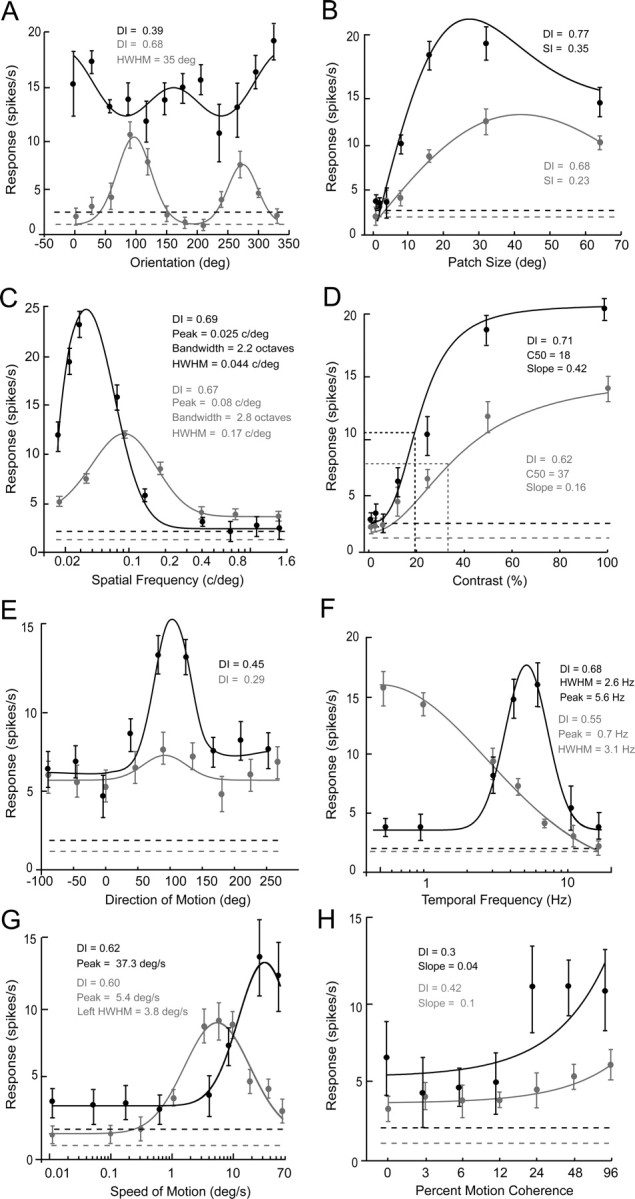
Distinct combinations of spatiotemporal response properties in two neurons recorded in layer 2/3 of mouse V1. A–H, Tuning curves of the spike discharge of the gray (60601c2) and the black (60302c2) neuron elicited by visually stimulating the receptive field. In each panel the mean response (±SE) is plotted as a function of the relevant stimulus variable. Each data point is the mean of 10 stimulus repetitions. The solid lines indicate the best fitting functions. The dashed lines indicate the average spontaneous activity when no stimulus was presented within the receptive field. SI denotes surround inhibition index. C₅₀ indicates the contrast at which the response magnitude is 50% of the peak. HWHM was measured on the left or the right side of the peak. Orientation (A), size (B), spatial frequency (C), contrast (D), and temporal frequency (F) tuning curves were obtained by stimulating with drifting sinusoidal gratings. Direction (E), speed (G), and coherence (H) tuning curves were obtained with moving random-dot stimuli. Notice that the gray neuron is optimally tuned to high spatial frequency, shows low contrast sensitivity, and prefers low temporal frequencies and slow speeds. In contrast, the black neuron is optimally tuned to low spatial frequency, is highly selective/sensitive to contrast, and prefers high temporal frequencies and fast speeds.

The tuning curves shown in black (Fig. 1) derive from a layer 2/3 neuron with a different set of response properties. Similar to the “gray neuron” the “black neuron” had a complex receptive field (F₁/F₀ = 0.23), but unlike in the gray cell the black cells' orientation tuning was nearly flat (DI = 0.39) (Fig. 1A), the size tuning showed robust surround inhibition (SI = 0.35) (Fig. 1B), the peak spatial frequency was low (0.025 c/deg) and the tuning bandwidth was narrow (2 octaves, corresponding to a linear range of 0.044 c/deg) (Fig. 1C), the contrast sensitivity was high (C₅₀ = 18%) (Fig. 1D), the direction selectivity was strong (DI = 0.59) (Fig. 1E), the temporal frequency tuning was bandpass (half-maximal bandwidth = 2.6 Hz) with a peak at 5.6 Hz (Fig. 1F), the speed tuning was broad (full bandwidth >55 deg/s) with a high peak velocity (37 deg/s) (Fig. 1G), and finally the neuron was relatively insensitive to motion coherence (Fig. 1H).

It is evident from these comparisons that the high spatial resolution neuron shown in gray (Fig. 1) responded to a four times broader range of spatial frequencies than the low spatial resolution neuron depicted in black (Fig. 1). In contrast, the low-spatial-frequency neuron shown in black was twice as sensitive to contrast, responded to a much broader range of speeds and peaked at an eightfold higher temporal frequency. Similar associations were found throughout the population of V1 neurons, whose response properties tended to follow one of two patterns: (1) high peak/broad bandwidth spatial frequency, low contrast selectivity (i.e., DI), low peak/narrow bandwidth temporal frequency, and low peak/narrow bandwidth speed tuning, or (2) low peak/narrow bandwidth spatial frequency, high contrast selectivity, high peak/broad bandwidth temporal frequency, and high peak/broad bandwidth speed tuning. Before discussing the conjunctive properties, we will first describe the responses to each stimulus parameter separately.

Spontaneous activity

The majority (75%) of neurons showed low spontaneous firing rates of <5 spikes/s (median: 2.7). Optimal stimulation of the receptive fields evoked maximal response rates of ∼40 spikes/s (median = 14.6). Neurons with high spontaneous firing rates generated significantly (ANOVA, p < 0.05) stronger responses. Unlike previous recordings in V1 of mouse and gray squirrel (Heimel et al., 2005; Niell and Stryker, 2008), we found no significant (R² = 0.025, p = 0.81) difference in spontaneous firing rates across cortical layers.

Latency

Latencies were extracted by pooling the responses to 10 repetitions of the optimal stimulus across five different tuning runs (i.e., orientation, spatial frequency, temporal frequency, contrast, size). Pooling a total of 50 responses across stimulus conditions and trials reduced the variance of the response and improved the accuracy with which we were able to determine the time point at which the firing rate increased significantly and consistently above background. Measured in this way, we found that the median onset latency of V1 responses was 110 ms (mean = 113 ± 2 ms) with 90% of neurons showing latencies in the range from 70 to 150 ms (Fig. 2A). The mean latency was ∼20 ms longer than those recorded in mouse LGN (Grubb and Thompson, 2003). Our latencies correspond well to latencies determined by VEP recordings in V1 (Porchiatti et al., 1999), and fall within the range found by current source density analyses in mouse V1 (Niell and Stryker, 2008). The mean latencies in layers 4, 5, and 6 were slightly shorter (108 ± 4 ms) than in layer 2/3 (116 ± 4 ms), but the difference narrowly escaped significance (p = 0.07). The similarities in onset latencies across different layers may not be surprising, given that all layers receive thalamocortical input (Antonini et al., 1999) and measurements in rat somatosensory cortex indicate that onset-latencies correlate more strongly with cell type than with laminar position (de Kock et al., 2007).

Figure 2.

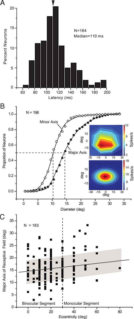
Response latencies and receptive field shape of V1 neurons. A, Distribution of response latency across all layers of V1. B, Cumulative histogram of major and minor axes of receptive fields in V1. Insets show heat maps of spike rate outlining a representative receptive field. Raw data (top), after smoothing with Gaussian function (bottom). C, Dependence of receptive field size (major axis) on eccentricity. Shading indicates SD.

Receptive field size

Receptive fields were mapped with small patches (5 deg) of drifting gratings flashed at different locations. The response fields were fit with a two-dimensional Gaussian and the contour corresponding to ±2 SD of the fitted Gaussian was taken as the receptive field. The receptive field size was determined by measuring the major and minor axes, computing the area of an ellipse, treating this area as circular and computing the diameter. These computations yielded a median receptive field size of 11.8 deg (mean 13.2 ± 0.3 deg) (see Fig. 4D), which closely corresponds to previous measurements (Métin et al., 1988; Niell and Stryker, 2008). Consistently, we found that the shapes of receptive fields were elliptical with significantly longer major (median = 14.7 deg) than minor axes (median = 10.8 deg) (Fig. 2B). In 90% of neurons the major axis of the receptive field was approximately aligned (± 20°) with the horizontal meridian. The length of the major axis significantly correlated (R² = 0.15, p = 0.03) with eccentricity, such that the mean length in the peripheral monocular segment (>30 deg eccentricity) was significantly (p = 0.007) greater (14.2 ± 0.5 deg) than in the central binocular segment (12.5 ± 0.3 deg) (Fig. 2C). The mean aspect ratio (1.4 ± 0.04), however, remained constant across different locations of the visuotopic map. The receptive fields in layers 5 and 6 were slightly larger (∼14 deg) than in layers 2/3 and 4 (∼12 deg), but the difference was not significant (p = 0.09).

Figure 4.

Size tuning of V1 neurons. A, Distribution of size DI across all V1 neurons (open bars), neurons with monotonically increasing or saturating tuning curves (gray bars), and surround-inhibited neurons (SI) are represented by black bars. Arrowheads with matching colors indicate median DI of the different groups of neurons. Solid arrow indicates DI of gray neuron shown in Figure 1B. Black arrow refers to neuron shown in Figure 1B. B, Distribution of optimal size. Inset shows representative examples of different size tuning curves: plateau (coarse dashes), monotonic (black), and surround inhibited (gray). The dashed line indicates the average spontaneous activity. C, Distribution of surround inhibition. D, Distribution of receptive field size. All conventions as in A.

Spatial summation

The responses of a small number of neurons were strongly modulated at the drift frequency of the grating stimulus (Fig. 3A), suggesting that receptive fields were composed of distinct subfields, which are characteristic features of simple cells (Hubel and Wiesel, 1962). Simple cells in cat V1 were shown to combine visual inputs across space and time in linear fashion (DeAngelis et al., 1993). To quantitatively determine the amount of relative modulation, we computed the ratio of the amplitude of the first harmonic of the response (F₁) and the mean spike rate (F₀). Previous studies in V1 of monkey, cat, gray squirrel and mouse have shown a bimodal distribution of F₁/F_0, in which ratios of >1 represent simple cells with linear spatial summation and values of <1 represent complex cells with nonlinear properties (Schiller et al., 1976; Skottun et al., 1991; Heimel et al., 2005; Niell and Stryker, 2008). However, because the F₁/F₀ ratio is a nonlinear metric, Mechler and Ringach (2002) have argued that it is inadequate for distinguishing simple and complex cells. Despite this complexity, we have used the F₁/F₀ ratio to compare our results with previous studies. Our analysis generally revealed that clear response modulation was lacking in cells with F₁/F₀ ratios of <1, but was present in spike raster plots and in normalized spike rate diagrams of responses with F₁/F₀ ratios of >1 (Fig. 3A,B). The distribution of the F₁/F₀ ratio was highly skewed with a median of 0.3 across the population, suggesting that the majority of V1 neurons had nonlinear summation properties, characteristic of complex receptive fields. Neurons with linear summation properties of simple cells were rare (6%, 14/211) and all of these cells were encountered in layers 2/3 and 4. This result is consistent with the previously reported paucity of neurons with linear response properties in deep layers of mouse V1 (Niell and Stryker, 2008).

Figure 3.

Spatial summation of V1 receptive fields. A, Raster plot showing the modulation of firing due to stimulation with a drifting sinusoidal grating (0.25 c/deg) at 2 Hz. B, Normalized spike frequency plot of the neuron shown in A. The cell shows linear summation properties with an F₁/F₀ ratio of 1.39. C, Distribution of F₁/F₀ across the population of V1 neurons. In the majority of neurons the F₁/F₀ ratio is <1, indicating nonlinear summation properties, a characteristic of complex cells. The median F₁/F₀ is indicated by an arrowhead. The gray arrow corresponds to the gray neuron shown in Figure 1. The black arrow refers to the black neuron shown in Figure 1.

Size tuning

We found that all neurons were significantly (ANOVA, p < 0.05) modulated by the size of a patch of drifting grating. To assess the size selectivity we computed a DI, which measures the ability of a neuron to distinguish changes in the stimulus relative to the intrinsic level of spiking variability. A DI of ≥0.425 typically corresponds to approximately a 2:1 or larger difference in maximal versus minimal firing rate and was reached by all neurons whose responses were significantly (ANOVA, p < 0.05) modulated by size. The median DI across the population was 0.67 (Fig. 4A). Size tuning curves showed 3 typical shapes over the range of stimulus sizes that we tested, which are illustrated by representative examples in the inset of Figure 4B. Cells for which responses reached a plateau (Fig. 4B, inset, cell 1) were most abundant (60.3%, 126/209) and had a median optimal size (defined as the size at which response reached 90% of maximum, corresponding to 1.163 α of the best-fit error function) of 33.3 deg (Fig. 4B). A smaller percentage (22.5%, 47/209) of cells showed responses that increased monotonically as a function of patch size (Fig. 4B, inset, cell 2), such that the largest size tested (64 deg) elicited the strongest response (Fig. 4B). The third group of cells showed nonmonotonic responses (Fig. 4B, inset, cell 3) that peaked at a median size of 27 deg and were significantly (p < 0.01) reduced by further increases in patch size. These surround inhibited neurons accounted for 17.2% (36/209) of size-tuned neurons. The median surround suppression for this group was 36%, which was significantly greater (p < 0.01) than that seen for plateau and monotonic neurons in which surround suppression was minimal or undetectable (Fig. 4C). Interestingly, the median size of the classical receptive field (as defined by the receptive field mapping approach described above) of plateau (13 deg), monotonic (11.5 deg) and surround inhibited neurons (10.9 deg) was significantly (p < 0.01) smaller than the patch size that elicited the optimal response (Fig. 4, D vs B). This suggests that plateau and monotonic neurons may have facilitatory surrounds or that substantial portions of their receptive fields produce subthreshold responses when probed with small stimuli as in our receptive field mapping test. By contrast, in surround inhibited neurons responses evoked from within the classical receptive field were suppressed by patches larger than 33 deg. No significant differences were found in the laminar (R² = 0.02, p = 0.57) and topographic (R² = 0.03, p = 0.68) distributions of the different types of size-tuned neurons.

Orientation tuning

The responses of approximately half (48.5%, 96/198) of neurons were significantly (ANOVA, p < 0.05) modulated by the orientation of drifting gratings. The degree of tuning varied from highly orientation selective (Fig. 1A, gray neuron) to nonselective (Fig. 1A, black neuron). This is expressed by a wide range of orientation DIs across the population (Fig. 5A). Most (92.7%, 89/96) orientation-selective neurons showed nonlinear spatial summation properties, whereas only 7.3% (7/96) were classified as linear based on the F₁/F₀ ratio. The median tuning width, measured as half width at half-maximal response, across the population of selectively tuned neurons was 43 degrees (Fig. 5B). Orientation-selective cells were found across layers 2/3–6 with no preferential laminar distribution of strength (R² = 0.05, p = 0.5) or width (R² = 0.07, p = 0.4) of tuning. There was no indication that specific orientations were preferentially distributed across the visual field (R² = −0.08, p = 0.28).

Figure 5.

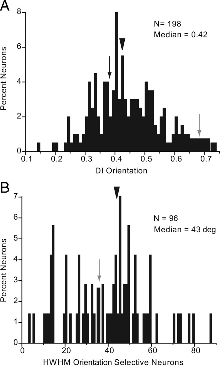
Orientation tuning of V1 neurons. A, Distribution of orientation DI. Median DI is indicated by arrowhead. Gray and black arrows indicate DIs of neurons shown in Figure 1A. B, Tuning bandwidth indicates the HWHM. Gray arrow refers to gray neuron in Figure 1A.

Spatial frequency tuning

All of the 207 neurons studied showed significant (ANOVA, p < 0.05) spatial frequency tuning to optimally oriented drifting gratings and had DIs of ≥0.425 (median = 0.63) (Fig. 6A). Representative examples shown in Fig. 1C demonstrate that different neurons had different peak sensitivities and tuning bandwidths. The optimal spatial frequency across the population ranged from 0.02 to 0.09 c/deg with a median of 0.03 c/deg (Fig. 6B). In 53% (110/207) of spatial-frequency-tuned neurons, the responses to the lowest frequency tested (0.015 c/deg) dropped significantly (p < 0.05) below half of the peak response, indicating that these neurons had bandpass properties and resembled the examples shown in Figure 1C. The remainder of tuning curves lacked a significant low-frequency rolloff and were therefore considered low pass. The median half bandwidth at half-maximal amplitude (on the high frequency side of the peak) was 0.044 c/deg (Fig. 6C). In 90% of neurons, responses decayed to 10% of maximum at or <0.43 c/deg, a point we defined as spatial frequency cutoff or neuronal spatial acuity. The median bandwidth for bandpass neurons was 2.23 octaves. Similar to monkey V1, in which responses to high spatial frequencies are more broadly tuned (on a linear scale) than responses to low spatial frequencies (De Valois et al., 1982), we found a significant positive correlation (R² = 0.39, p < 0.0001) between peak spatial frequency and spatial frequency cutoff (Fig. 6D). The tuning bandwidths of neurons in deep layers 5 and 6 were significantly (p < 0.05) broader than in more superficial layers, which is consistent with the findings of Niell and Stryker (2008). In contrast, we found no significant (R² = −0.08, p = 0.21) correlation between tuning bandwidth and visual field eccentricity.

Figure 6.

Spatial frequency tuning of V1 neurons. A, Distribution of spatial frequency DI across V1 neurons. Arrowhead indicates median DI. Gray and black arrows indicate DIs of neurons shown in Figure 1C. B, Distribution of peak spatial frequency. Conventions as in A. C, Distribution of spatial frequency bandwidth indicated by HWHM. Conventions as in A. D, Positive significant (R² = 0.39, p < 0.0001) correlation between tuning bandwidth and spatial frequency cutoff.

Contrast–response functions

Contrast selectivity and sensitivity was examined with drifting sinusoidal gratings at the cells' optimal orientation, spatial frequency, temporal frequency, and direction. The results show that the responses of all 198 neurons tested were significantly (ANOVA, p < 0.05) modulated by grating contrast and that the median DI across the population was 0.63 (Fig. 7A). Every contrast–response function resembled a hyperbolic curve that saturated at 100% contrast and was well fit with a Naka–Rushton (Naka and Rushton, 1966) function (Fig. 1D). To quantify contrast sensitivity we plotted the C₅₀, which is the contrast at which the response reached 50% of the peak. Figure 7B shows that the median C₅₀ across the population was 38.4%. The examples illustrated in Figure 1D show that the slope of the best-fitting function varied substantially in steepness (slope of gray neuron = 0.16; slope of black neuron = 0.42), suggesting that cells with high contrast sensitivity have a higher gain than cells with low contrast sensitivity, which are superior in detecting small increments in stimulus contrast. The distribution of C₅₀ across layers and eccentricities was not significantly (R² = −0.03, p = 0.64; R² = 0.03, p = 0.68; respectively) different from uniform.

Figure 7.

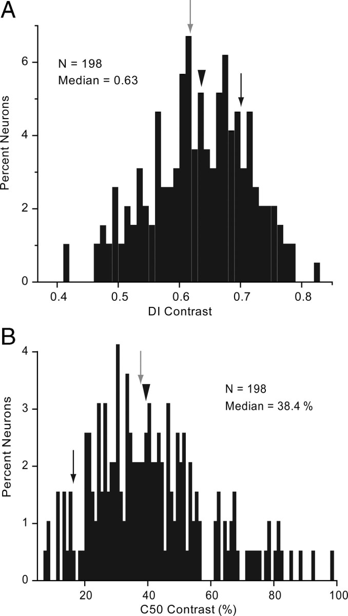
Contrast tuning of V1 neurons. A, Distribution of contrast DI. Arrowhead indicates median DI. Gray and black arrows points to DI of neurons shown in Figure 1D. B, Distribution of percentage contrast that elicits half-maximal response (C₅₀). Conventions as in A.

Direction tuning

Direction tuning was examined with moving random-dot patterns. We found that these stimuli effectively activated V1 neurons and revealed a small number of cells that were highly selective to the direction of stimulus motion (Fig. 1E, black neuron). Most cells, however, showed no significant tuning (Fig. 1E, gray neuron). In fact, across the population, significant (ANOVA, p < 0.05) direction tuning was rare and observed in only 7% (14/198) of neurons, just slightly more common than expected by chance. The scarcity of direction-selective neurons in V1 was reflected by a low median DI of 0.3 (Fig. 8A). Because the peak activation rate with moving dots was often relatively low we additionally assessed direction selectivity with drifting gratings. “Grating-direction-selective” neurons showed responses to movements opposite to the optimal direction that were significantly (t test, p < 0.05) lower and indistinguishable from background. Even under these stimulation conditions, only a small number (6%, 12/198) of neurons showed significant direction tuning. Two of these neurons were tuned for both the direction of moving gratings and random dots. The rest of the grating-direction-selective neurons were indifferent to the direction of moving dots. One of these neurons is shown in Figure 8B. Together both populations accounted for a total of 12% direction-selective neurons. Similar to the results of Niell and Stryker (2008), most (77%, 17/22) direction-selective neurons were found in layer 2/3 and had a median tuning full width at half-maximal amplitude of 80.6 deg. The distribution of direction-selective neurons across different eccentricities of the visual field was approximately flat.

Figure 8.

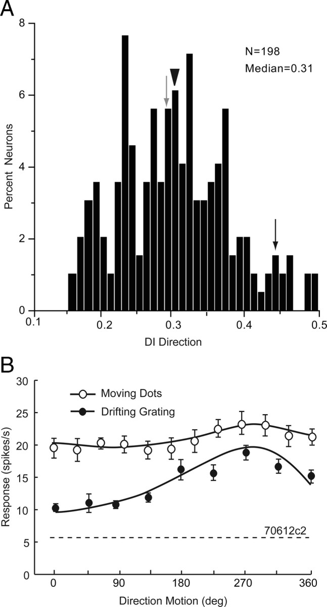
Direction tuning of V1 neurons. A, Distribution of direction tuning DI. Arrowhead indicates median DI. Gray and black arrows point to DIs of neurons shown in Figure 1E. B, Representative example of direction tuning to moving random-dot pattern (black dots). The same neuron shows a flat direction tuning curve to moving sinusoidal grating (white dots). Stippled line indicates spontaneous firing rate.

Temporal frequency tuning

More than 90% (192/212) of V1 neurons were significantly tuned to the temporal frequency of optimally oriented drifting gratings (Fig. 1F) and showed a high median DI of 0.6 (Fig. 9A). Approximately 44% (84/192) of neurons showed low-pass properties, in which the responses to the lowest frequencies did not drop significantly (p < 0.05) below half of the peak response. In this population, the median optimal response (1.2 Hz) coincided with the lowest temporal frequency tested or peaked near the minimum (Fig. 9B). The remaining 56% (108/192) of neurons had bandpass properties (i.e., the response to the lowest frequency was significantly (p < 0.05) less than half of the peak) similar to the black cell shown in Figure 1F. The median peak temporal frequency of these neurons was 1.9 Hz, which was significantly (p < 0.001) higher than the 1.2 Hz found in low-pass neurons. In addition, we found that bandpass neurons tended to be tuned to a broader range of temporal frequencies (median half-width at half-maximal amplitude = 3.6 Hz) than low-pass neurons (median half-width = 2.9 Hz), although the difference was not significant (p = 0.12) (Fig. 9C). Cells with low temporal frequency peaks had significantly (R² = 0.37, p < 0.0001) narrower bandwidths than cells that preferred higher temporal frequencies (Fig. 9D). Deep-layer neurons (layers 5, 6) had significantly (p < 0.003) broader temporal frequency bandwidths (median = 3.5 Hz) than cells in layers 2/3 and 4 (median = 2.7 Hz. The tuning bandwidth was significantly (R² = 0.15, p = 0.035) higher at more eccentric locations within the visual field.

Figure 9.

Temporal frequency tuning of V1 neurons. A, Distribution of temporal frequency DI. Arrowhead indicates median DI. Gray and black arrows indicate DIs of neurons shown in Figure 1F. B, Peak temporal frequency of low-pass (black bars, black arrowhead indicates median) and bandpass (gray bars, gray arrowhead indicates median) neurons. Conventions as in A. C, Distribution of temporal frequency bandwidth indicated by the HWHM. Low-pass neurons and median HWHM are shown in black. Bandpass neurons are represented in gray. Conventions as in A. D, Positive significant (R² = 0.37, p < 0.0001) correlation of temporal frequency HWHM and peak temporal frequency.

Speed tuning

Almost half of V1 neurons (45.3%, 92/203) were significantly (ANOVA, p < 0.05) tuned to the speed of moving random-dot patterns. The median DI (0.4), however, was relatively low (Fig. 10A). The speed tuning curves showed low-pass (i.e., response to lowest speed >50% of peak response), bandpass (Fig. 1G, gray neuron), and high-pass (Fig. 1G, black neuron) (i.e., response to highest speed >50% of peak) properties. Additional examples of these 3 types of tuning are illustrated in the inset of Fig. 10B. Low-pass neurons (Fig. 10B, cell 1) were rare (5.4%, 5/92) and most cells showed either bandpass (Fig. 10B, cell 2) (45.6%, 42/92) or high-pass (Fig. 10B, cell 3) (49%, 45/92) properties over the range of speeds we tested. The median optimal speed across the population of tuned neurons was 10.6 deg/s (Fig. 10B). Low-pass neurons peaked at a median speed of 0.5 deg/s, bandpass cells had significantly (p < 0.001) higher median peak speeds of 6.6 deg/s, whereas high-pass neurons registered an optimal median speed of 33.8 deg/s. To compare the speed tuning bandwidth of bandpass and high-pass neurons, we determined the half-maximal bandwidth on the left side of the peak (L-HWHM). We found that the median L-HWHM across the population of bandpass neurons was 5 deg/s. By contrast, high-pass neurons showed a significantly (p < 0.0001) broader median L-HWHM of 24.6 deg/s (Fig. 10C). Peak speed and tuning bandwidth tended to be higher in deep than superficial layers, but the differences were not significant. Similarly, we found no significant differences in speed tuning across different eccentricities of the visuotopic map.

Figure 10.

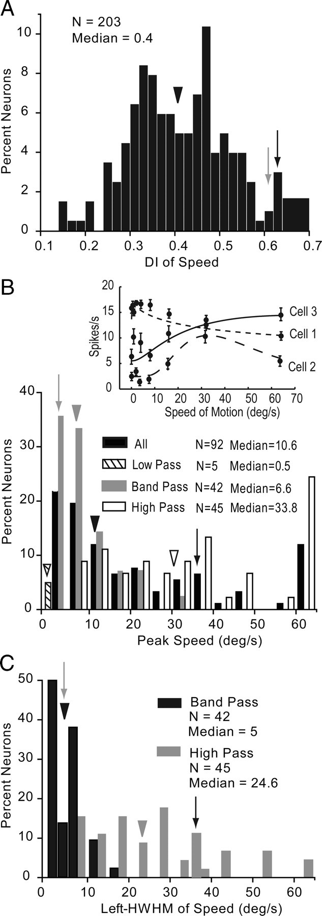
Speed tuning of V1 neurons. A, Distribution of speed DI. Arrowhead indicates median DI. Gray and black arrows indicate DIs of neurons shown in Fig. 1G. B, Peak speed of all (black bars), low-pass (hatched bars), bandpass (gray bars), and high-pass (white bars) neurons. Arrowhead with matching patterns indicates median across the respective population. Conventions as in A. C, Distribution of speed bandwidth indicated by the L-HWHM. Bandpass neurons (black bars) and high-pass neurons (gray bars) are shown. Conventions as in A.

Motion coherence tuning

To determine the strength of motion tuning, we used translating moving random-dot displays in which motion strength was varied independently of positional and form cues (Britten et al., 1992). This was achieved by varying the percentage of dots that are repositioned with a fixed spatial offset at a fixed rate, thereby changing the degree by which dots move coherently in a particular direction. We found that a substantial number of V1 neurons responded monotonically as a function of motion energy, by firing more strongly when the dots moved with 100% coherence than when they moved at random (Fig. 1H, black neuron). Across the population, 35.7% (70/196) of V1 neurons were significantly (ANOVA, p < 0.05) modulated by coherence and 27.5% (54/196) of neurons reached DIs of ≥0.425 (Fig. 11A). The median slope of tuning was shallow (median = 0.04) and in the vast majority of cases was positively inclined (Fig. 11B). Only two coherence-selective neurons showed negative slopes (Fig. 11B), indicating that responses were attenuated by higher degrees of coherence. Negatively sloped coherence tuning curves were previously observed in monkey, when direction-selective MT neurons were stimulated with random-dot displays moving in the nonpreferred direction (Britten et al., 1993). In mouse V1, however, both of the negatively sloped neurons were not significantly direction selective. In fact, direction selectivity was rare in coherence-tuned neurons (6/70, 8.5%). Of the few neurons that were both direction and coherence selective, the responses in the nonpreferred direction were smaller but constant across all coherences. Thus, the majority of coherence-tuned neurons appeared to be selective for the strength of motion but was indifferent to the direction of movement. Coherence-tuned neurons were found across all layers, but the sample is too small to comment on the laminar distribution.

Figure 11.

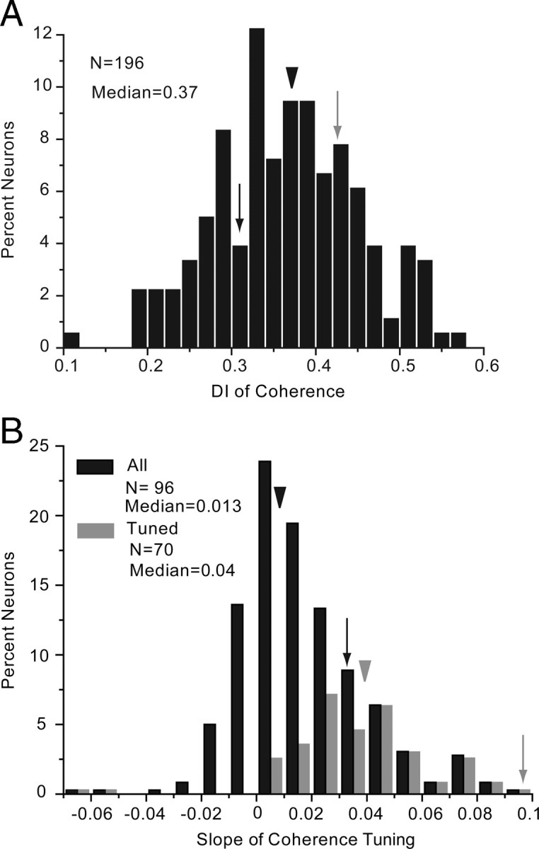
Motion coherence tuning in V1. A, Distribution of coherence DI. Arrowhead indicates median DI. Gray and black arrows indicate DIs of the neurons shown in Figure 1H. B, Distribution of slope of coherence tuning derived from linear fits of the tuning curves. Black bars represent all neurons. Gray bars represent coherence-tuned neurons. Black and gray arrowheads indicate median DI for the corresponding populations, all other conventions as in A.

Tuning to combinations of features

Niell and Stryker (2008) have shown that mouse V1 neurons are highly selective along multiple stimulus dimensions. If the visual inputs that give rise to these receptive field properties reach V1 through parallel channels with distinct spatiotemporal properties, one might expect to find that neurons with short latencies are highly sensitive to contrast, have large receptive fields, and prefer fast-changing, low-spatial-frequency stimuli (Kaplan, 2008). Thus, we were interested in whether single neurons are optimally tuned to specific combinations of features. To study such relationships, we performed regression analyses with latency, receptive field size, and sensitivities to contrast, temporal frequency, speed, and spatial frequency as variables.

Short-latency neurons encode transient stimuli

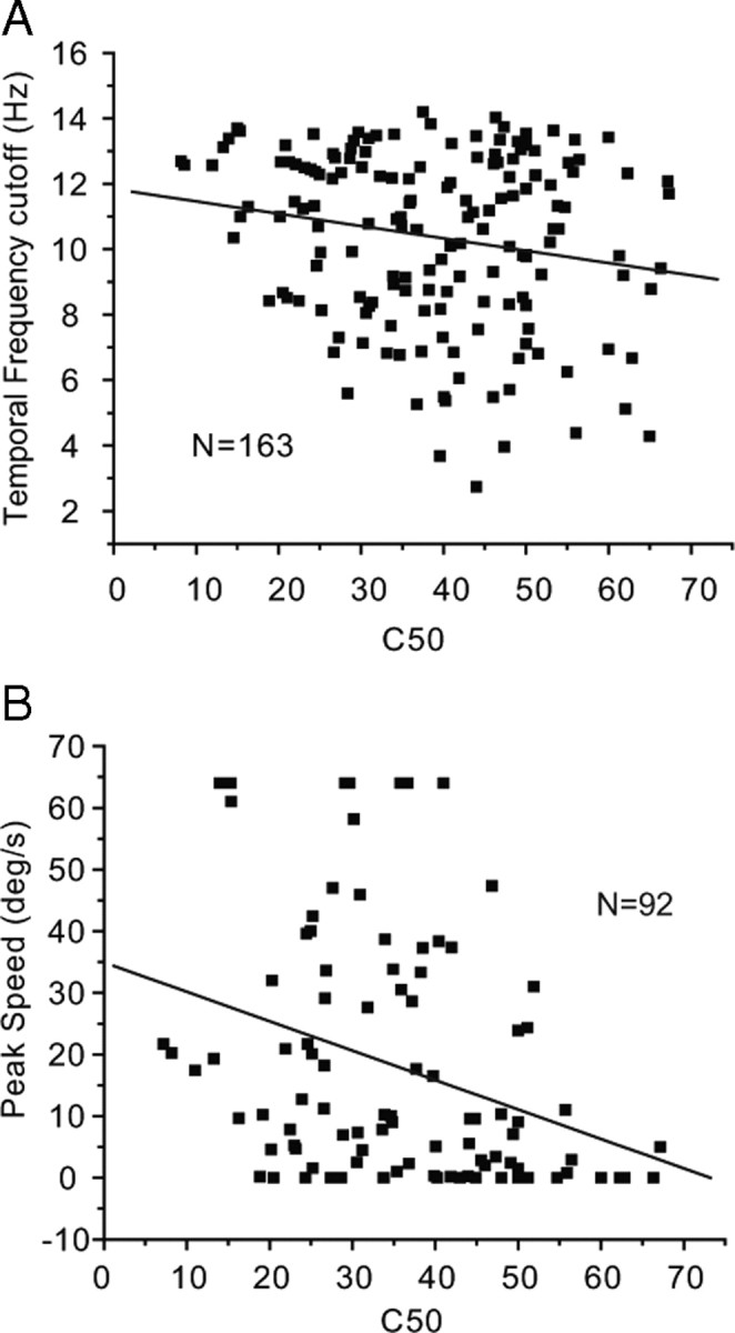
Our correlation analyses showed that neurons with short onset latency had significantly (R² = 0.31, p < 0.0001) higher contrast sensitivities (i.e., lower C₅₀) than neurons with longer latencies (Fig. 12A). In addition, we found that neurons with short latencies had significantly (R² = −0.28, p = 0.005) higher temporal frequency cutoffs (Fig. 12B) and responded to significantly (R² = −0.31, p = 0.005) higher peak speeds (Fig. 12C). Interestingly, short-latency neurons preferred significantly (R² = 0.34, p < 0.0001) lower spatial frequencies (Fig 12D), indicating that neurons with low spatial acuity have faster response times.

Figure 12.

Correlations of contrast, temporal frequency, speed, and spatial frequency tuning with onset latency in V1. A, Short-latency neurons have significantly (R² = 0.31, p < 0.001) higher contrast sensitivity (i.e., low C₅₀). B, Short-latency neurons have significantly (R² = −0.28, p = 0.005) higher temporal frequency cutoff. C, Short-latency neurons are optimally tuned to significantly (R² = −0.31, p = 0.005) higher speeds. D, Short-latency neurons have significantly (R² = 0.34, p < 0.0001) lower spatial frequency cutoff.

Studies in monkey, cat, and gray squirrel LGN have found that short-latency neurons have larger receptive fields (Shapley and Perry, 1986; Usrey and Reid, 2000; Van Hooser et al., 2003; Weng et al., 2005). In agreement with previous studies in rat LGN (Hale et al., 1979; Gabriel et al., 1996), we found no evidence for such a relationship (R² = −0.08, p = 0.3) in mouse V1 (supplemental Fig. 1A, available at www.jneurosci.org as supplemental material).

Transient stimuli are encoded by neurons with high contrast sensitivity

Our correlation analyses have shown that neurons with high contrast sensitivity (i.e., low C₅₀) have significantly (R² = −0.19, p = 0.015) higher temporal frequency cutoffs than neurons with low contrast sensitivity (Fig. 13A). A similar significant (R² = −0.32, p = 0.001) negative correlation was found between C₅₀ and peak speed (Fig. 13B), suggesting that highly contrast-sensitive neurons are optimally tuned to high speeds of visual motion.

Figure 13.

Correlations between contrast sensitivity, temporal frequency, and speed cutoff in V1. A, Neurons with higher contrast sensitivity (i.e., low C₅₀) have significantly (R² = 0.19, p = 0.015) higher temporal frequency cutoff. B, Neurons with higher contrast sensitivity are optimally tuned to significantly (R² = −0.32, p = 0.001) higher speeds.

Recordings in cat and monkey LGN have found that highly contrast-sensitive neurons have larger receptive fields (Shapley and Perry, 1986; Usrey and Reid, 2000; Weng et al., 2005). We have found no evidence for such a relationship (R² = −0.01, p = 0.88) in mouse V1 (supplemental Fig. 1B, available at www.jneurosci.org as supplemental material).

High spatial frequencies are encoded by neurons with low contrast sensitivity and a preference for sustained stimuli

Previous recordings in cat visual cortex have reported two classes of neurons: one that prefers high spatial frequencies and low temporal frequencies and another that is optimally tuned to low spatial frequencies and high temporal frequencies (Movshon et al., 1978). Recordings in cat area 18 have further shown that neurons with high spatial acuity prefer slower speeds (Bisti et al., 1985). Our correlation analyses in mouse V1 have shown that the spatial frequency cutoff was significantly (R² = 0.17, p = 0.03) positively correlated with C₅₀ (Fig. 14A), suggesting that low spatial acuity neurons have higher contrast sensitivity than neurons with high spatial acuity. In addition, we found that the spatial frequency cutoff was significantly negatively correlated with the temporal frequency cutoff (R² = −0.27, p = 0.0002) (Fig. 14B) and peak speed (R² = −0.25, p = 0.02) (Fig. 14C), suggesting that neurons with low spatial acuity prefer higher temporal frequencies and faster speeds whereas high-spatial-frequency neurons prefer slowly moving stimuli. Peak speed was positively correlated (R² = −0.49, p < 0.0001) with peak temporal frequency (Fig. 14D), which is consistent with the notion that speed preference is inversely proportional to spatial frequency (Priebe et al., 2006).

Figure 14.

Correlations between spatial frequency, contrast sensitivity, temporal frequency, and speed in V1. A, Neurons with higher spatial frequency cutoff have significantly (R² = 0.17, p = 0.03) lower contrast sensitivity (i.e., high C₅₀). B, Neurons with higher spatial frequency cutoff have significantly (R² = −0.27, p = 0.002) lower temporal frequency cutoff. C, Neurons with higher spatial frequency cutoff are optimally tuned to significantly (R² = −0.25, p = 0.02) lower peak speeds. D, Neurons that are tuned to higher peak temporal frequencies prefer significantly (R² = 0.49, p < 0.0001) higher speeds.

Because orientation and spatial acuity are important determinants of texture and contour discrimination (Burr and Wijesundra, 1991), we were interested whether the orientation selectivity index was correlated with the spatial frequency cutoff. Although we found some neurons in which both parameters were associated (Fig. 1A,C, gray cell), the correlation across the population of neurons was not significant (data not shown).

Discussion

In primates, visual input to the brain is carried in parallel channels specialized for processing spatial and temporal information (DeYoe and Van Essen, 1988; Nassi and Callaway, 2009). We found that in mouse V1, neurons with short response latencies have low spatial acuity and high sensitivity to contrast, temporal frequency, and speed, whereas neurons with long latencies have high spatial acuity, low sensitivities to contrast, temporal frequency, and speed. These correlations demonstrate that V1 neurons receive inputs from a weighted combination of parallel afferent pathways and suggest that the visual processing strategy of primates is conserved in the mouse visual system.

Elongated receptive fields with modulatory surrounds

We found that receptive fields are horizontally elongated and approximately match the shape and topography of geniculocortical axons (Antonini et al., 1999). This geometry is constant across the visuotopic map while receptive field size increases with eccentricity, supporting the notion of a parallel reduction in cortical magnification (Kalatsky and Stryker, 2003).

Many neurons show increasing responses with the size of grating patches well beyond the dimensions of the classical receptive field, as mapped with small stimuli. Similar observations were made in monkey V1 (Angelucci et al., 2002), suggesting that receptive fields are larger than geniculocortical axon arbors (Angelucci and Sainsbury, 2006) and involve additional inputs from intracortical networks (Angelucci and Bressloff, 2006). In neurons, with saturating and monotonically increasing size tuning curves, these converging inputs may arise from lateral connections within V1 that span 60 deg of the visuotopic map. Such connections are known to exist in many species including rat and squirrel (Burkhalter and Charles, 1990; Rumberger et al., 2001; Van Hooser et al., 2006) and may also be present in mouse V1.

Almost 20% of responses are suppressed by stimuli larger than the classical receptive field. The incidence of surround suppression is similar to that in squirrel V1 (Van Hooser et al., 2006), but is lower than in rat, cat, and macaque (DeAngelis et al., 1992; Girman et al., 1999; Sceniak et al., 2001). These center/surround interactions suggest that rodent V1 contains the machinery for identifying orientation contrasts and/or contour integration, which is necessary for object recognition (Zoccolan et al., 2009).

Orientation

We found that 48% of V1 neurons are orientation selective. The percentage is higher than the 32–41% observed earlier qualitative studies (Dräger, 1975; Mangini et al., 1980; Métin et al., 1988), but is lower than the 74% found in the quantitative analysis by Niell and Stryker (2008). Unlike all other studies, Niell and Stryker (2008) used multisite recordings and distinguished pyramidal from nonpyramidal cells, which enabled sampling of a broader spectrum of neurons with greater selectivity than traditional approaches. The advantages are evident in significant laminar differences of several properties including orientation selectivity (Niell and Stryker, 2008), which were less apparent in our study. Thus, recordings with tungsten electrodes may have biased against thin layers and small neurons, and favored complex cells, whose responses are more vigorous than those of simple cells (Martin and Whitteridge, 1984; Skottun et al., 1988; Hirsch et al., 2003). Indeed, our sample contained only 6% linear neurons (simple cells), which is much less than the 48% recorded by Niell and Stryker (2008). A similar bias for complex cells was observed in squirrel V1 (Heimel et al., 2005). Interestingly, Niell and Stryker (2008) found that only 31% of nonlinear neurons are orientation selective. This is less than the 45% orientation selectivity we have found among nonlinear neurons, suggesting that our lower percentage is not a detection issue, but is due preferential sampling of complex cells. Biased sampling of nonlinear responses with tungsten microelectrodes was observed previously in cat LGN (So and Shapley, 1979).

Direction

Previous recordings in mouse, rat, rabbit and macaque found that 24–38% of V1 neurons were direction selective for moving bars and gratings (Chow et al., 1971; Dräger, 1975; Schiller et al., 1976; Métin et al., 1988; Girman et al., 1999; Niell and Stryker, 2008). Using drifting grating and random-dot stimuli together, we found that only 12% of mouse V1 neurons are direction tuned, which is more than reported by Mangini and Pearlman (1980) but less than the 38% observed by Niell and Stryker (2008). A likely reason for the difference is that most of our recordings are from complex cells, which in squirrel V1 tend to be nondirectional (Heimel et al., 2005). This may be the result of preferential channeling of direction-selective signals from the retina (Huberman et al., 2008, 2009; Kim et al., 2008) to simple cells in V1 (Hoffman and Stone, 1971; Singer et al., 1975; Ferster and Lindström, 1983).

Motion coherence

Previous recordings in cat have shown that V1 neurons are modulated by the coherence of moving dots (Shumikhina et al., 2004). We found that 27.5% of mouse V1 neurons have similar properties. Unlike in monkey MT in which most coherence modulated neurons are direction selective (Britten et al., 1993), such neurons account for <3% in mouse V1. This suggests that mice that are able to discriminate the direction of moving random dots (Douglas et al., 2006), either rely on very few V1 neurons, or that coherence modulated direction-selective neurons are more abundant outside of V1.

Spatial frequency

Similar to Niell and Stryker (2008), we found that the median spatial frequency response peaks at 0.03 c/deg. Our data further show that in 90% of neurons the cutoff spatial frequency is ≤0.43 c/deg and approximately matches the behaviorally determined visual acuity (0.48–0.55 c/deg; Prusky and Douglas, 2004; Umino et al., 2008), supporting the role of V1 in high acuity vision (Prusky and Douglas, 2004).

Temporal frequency

Ninety percent of V1 responses are temporal frequency tuned and peak at 1–2 Hz, as shown previously by Niell and Stryker (2008). Similar to findings in monkey (Hawken et al., 1996), the peak temporal frequency in V1 is lower than in the LGN (4 Hz; Grubb and Thompson, 2003). In addition, mouse LGN neurons were shown to be bandpass for temporal frequency (Grubb and Thompson, 2003). In contrast, we found both low-pass and bandpass neurons in V1. These results suggest that in a subset of neurons bandpass temporal frequency tuning is transformed into low-pass tuning and as a result V1 neurons acquire properties that match the sensitivity of mouse photopic vision (Umino et al., 2008).

Speed

Similar to previous studies in cat and monkey V1 (Cao and Schiller, 2003; Price et al., 2006), we found that the optimal speed sensitivity in mouse V1 is ∼10 deg/s. However, due to technical limitations we have not examined speeds of >64 deg/s, suggesting that the average peak speed may be higher and may exceed the 50 deg/s recorded in rat V1 (Girman et al., 1999).

The speed of stimulus motion corresponds to the ratio of temporal and spatial frequency. In mice, speed discrimination was found to be independent of spatial frequency (Umino et al., 2008), suggesting that the mouse visual system contains truly speed-selective neurons. Because we have not measured responses of single neurons as a function of both temporal and spatial frequency, it remains unresolved whether such neurons exist in V1.

Parallel channels

We found that neurons with short response times and high contrast sensitivity are more sensitive to fast-changing, rapidly moving stimuli than long-latency neurons, which have low contrast sensitivity and high spatial resolution. Although these correlations are highly significant, they account for maximally 39% of the variance across the population, indicating that a substantial number of neurons have only weak preferences for particular combinations of spatiotemporal visual features. The extremes, however, suggest that high spatial and temporal sensitivity signals are carried to V1 in parallel channels similar to those of high-acuity visual systems (Stone et al., 1979; Van Hooser and Nelson, 2006; Nassi and Callaway, 2009). In contrast, recordings in mouse LGN showed little evidence for parallel processing, but revealed a trend in which short-latency ON-center neurons had higher contrast sensitivity and peak temporal frequencies (Grubb and Thompson, 2003). Although Grubb and Thompson (2003) identified separate groups of mouse LGN neurons with sustained and transient responses, the tuning was similar in all other respects. Comparisons of single response parameters further revealed distinct groups of rat LGN neurons, with inputs from optic tract fibers with different conduction velocities and different spatial summation properties (Hale et al., 1979; Lennie and Perry, 1981). The most complete evidence for physiologically distinct X (homologous to P), Y (homologous to M), and W channels in the rodent geniculocortical system, however, derives from recordings in squirrel LGN, in which short-latency neurons with transient responses have lower spatial resolution and greater contrast sensitivity than neurons with sustained responses and long latencies (Van Hooser et al., 2003). Our results are consistent with this organization and suggest that sensory cues carried by parallel channels are integrated in various balances and encode diverse temporal, contrast and spatial sensitivities in neurons across V1. Thus, the basic plan of the mouse visual system is remarkably similar to that of primates.

References

- Albrecht DG, Hamilton DB. Striate cortex of monkey and cat: contrast response function. J Neurophysiol. 1982;48:217–237. doi: 10.1152/jn.1982.48.1.217. [DOI] [PubMed] [Google Scholar]
- Angelucci A, Bressloff PC. Contribution of feedforward, lateral ad feedback connections to the classical receptive field center and extra-classical receptive field surround of primate V1 neurons. Prog Brain Res. 2006;154:93–120. doi: 10.1016/S0079-6123(06)54005-1. [DOI] [PubMed] [Google Scholar]
- Angelucci A, Sainsbury K. Contribution of feedforward thalamic afferents and corticogeniculate feedback to the spatial summation area of macaque V1 and LGN. J Comp Neurol. 2006;498:330–351. doi: 10.1002/cne.21060. [DOI] [PubMed] [Google Scholar]
- Angelucci A, Levitt JB, Walton EJ, Hupe JM, Bullier J, Lund JS. Circuits for local and global signal integration in primary visual cortex. J Neurosci. 2002;22:8633–8646. doi: 10.1523/JNEUROSCI.22-19-08633.2002. [DOI] [PMC free article] [PubMed] [Google Scholar]
- Antonini A, Fagiolini M, Stryker MP. Anatomical correlates of functional plasticity in mouse visual cortex. J Neurosci. 1999;19:4388–4406. doi: 10.1523/JNEUROSCI.19-11-04388.1999. [DOI] [PMC free article] [PubMed] [Google Scholar]
- Bisti S, Carmignoto G, Galli L, Maffei L. Spatial-frequency characteristics of neurons of area 18 in the cat: dependence on the velocity of the visual stimulus. J Physiol. 1985;359:259–268. doi: 10.1113/jphysiol.1985.sp015584. [DOI] [PMC free article] [PubMed] [Google Scholar]
- Britten KH, Shadlen MN, Newsome WT, Movshon JA. The analysis of visual motion: a comparison of neurons and psychophysical performance. J Neurosci. 1992;12:4745–4765. doi: 10.1523/JNEUROSCI.12-12-04745.1992. [DOI] [PMC free article] [PubMed] [Google Scholar]
- Britten KH, Shadlen MN, Newsome WT, Movshon JA. Responses of neurons in macaque MT to stochastic motion signals. Vis Neurosci. 1993;10:1157–1169. doi: 10.1017/s0952523800010269. [DOI] [PubMed] [Google Scholar]
- Burkhalter A, Charles V. Organization of local axon collateral of efferent projection neurons in rat visual cortex. J Comp Neurol. 1990;302:920–934. doi: 10.1002/cne.903020417. [DOI] [PubMed] [Google Scholar]
- Burr DC, Wijesundra SA. Orientation discrimination depends on spatial frequency. Vision Res. 1991;31:1449–1452. doi: 10.1016/0042-6989(91)90064-c. [DOI] [PubMed] [Google Scholar]
- Cao A, Schiller PH. Neuronal responses to relative speed in primary visual cortex of rhesus monkey. Vis Neurosci. 2003;20:77–84. doi: 10.1017/s0952523803201085. [DOI] [PubMed] [Google Scholar]
- Chow KL, Masland RH, Stewart DL. Receptive field characteristics of striate cortical neurons in the rabbit. Brain Res. 1971;33:337–352. doi: 10.1016/0006-8993(71)90107-7. [DOI] [PubMed] [Google Scholar]
- DeAngelis GC, Uka T. Coding of horizontal disparity and velocity by MT neurons in the alert macaque. J Neurophysiol. 2003;89:1094–1111. doi: 10.1152/jn.00717.2002. [DOI] [PubMed] [Google Scholar]
- DeAngelis GC, Robson JG, Ohzawa I, Freeman RD. Organization of suppression in receptive field of neurons in cat visual cortex. J Neurophysiol. 1992;68:144–163. doi: 10.1152/jn.1992.68.1.144. [DOI] [PubMed] [Google Scholar]
- DeAngelis GC, Ohzawa I, Freeman RD. Spatiotemporal organization of simple-cell receptive fields in the cat's striate cortex. II. Linearity of temporal and spatial summation. J Neurophysiol. 1993;69:1118–1135. doi: 10.1152/jn.1993.69.4.1118. [DOI] [PubMed] [Google Scholar]
- de Kock CP, Bruno RM, Spors H, Sakmann B. Layer- and cell-type-specific suprathreshold stimulus representation in rat primary somatosensory cortex. J Physiol. 2007;581:139–154. doi: 10.1113/jphysiol.2006.124321. [DOI] [PMC free article] [PubMed] [Google Scholar]
- De Valois RL, Morgan H, Snodderly DM. Psychophysical studies of monkey vision. 3. Spatial luminance contrast sensitivity tests of macaque and human observers. Vision Res. 1974;14:75–81. doi: 10.1016/0042-6989(74)90118-7. [DOI] [PubMed] [Google Scholar]
- De Valois RL, Albrecht DG, Thorell LG. Spatial frequency selectivity of cells in macaque visual cortex. Vision Res. 1982;22:545–559. doi: 10.1016/0042-6989(82)90113-4. [DOI] [PubMed] [Google Scholar]
- DeYoe EA, Van Essen DC. Concurrent processing streams in monkey visual cortex. Trends Neurosci. 1988;11:219–226. doi: 10.1016/0166-2236(88)90130-0. [DOI] [PubMed] [Google Scholar]
- Douglas RM, Neve A, Quittenbaum JP, Alam NM, Prusky GT. Perception of visual motion coherence by rats and mice. Vision Res. 2006;46:2842–2847. doi: 10.1016/j.visres.2006.02.025. [DOI] [PubMed] [Google Scholar]
- Dräger UC. Receptive fields of single cells and topography in mouse visual cortex. J Comp Neurol. 1975;160:269–290. doi: 10.1002/cne.901600302. [DOI] [PubMed] [Google Scholar]
- Dräger UC, Olsen JF. Origins of crossed and uncrossed retinal projections in pigmented and albino mice. J Comp Neurol. 1980;191:383–412. doi: 10.1002/cne.901910306. [DOI] [PubMed] [Google Scholar]
- Draper NR, Smith H. Advanced regression analysis. New York: Wiley; 1966. [Google Scholar]
- Ferster D, Lindström S. An intracellular analysis of geniculo-cortical connectivity in area 17 of the cat. J Physiol. 1983;342:181–215. doi: 10.1113/jphysiol.1983.sp014846. [DOI] [PMC free article] [PubMed] [Google Scholar]
- Fukuda Y. Differentiation of principal cells of the rat lateral geniculate body into two groups: fast and slow cells. Exp Brain Res. 1973;119:327–344. doi: 10.1007/BF00234664. [DOI] [PubMed] [Google Scholar]
- Gabriel S, Gabriel HJ, Zippel U, Brandl H. Regional distribution of fast and slow geniculo-cortical relay cells (GCR-cells) within the rat's dorsal lateral geniculate nucleus (LGNd) Exp Brain Res. 1985;61:210–213. doi: 10.1007/BF00235637. [DOI] [PubMed] [Google Scholar]
- Gabriel S, Gabriel HJ, Grützmann R, Berlin K, Davidowa H. Effects of cholecystokinin on Y, X, and W cells in the dorsal lateral geniculate nucleus of rats. Exp Brain Res. 1996;109:43–55. doi: 10.1007/BF00228625. [DOI] [PubMed] [Google Scholar]
- Girman SV, Sauvé Y, Lund RD. Receptive field properties of single neurons in rat primary visual cortex. J Neurophysiol. 1999;82:301–311. doi: 10.1152/jn.1999.82.1.301. [DOI] [PubMed] [Google Scholar]
- Gordon JA, Stryker MP. Experience-dependent plasticity of binocular responses in the primary visual cortex of the mouse. J Neurosci. 1996;16:3274–3286. doi: 10.1523/JNEUROSCI.16-10-03274.1996. [DOI] [PMC free article] [PubMed] [Google Scholar]
- Grubb MS, Thompson ID. Quantitative characterization of visual response properties in the mouse dorsal lateral geniculate nucleus. J Neurophysiol. 2003;90:3594–3607. doi: 10.1152/jn.00699.2003. [DOI] [PubMed] [Google Scholar]
- Hale PT, Sefton AJ, Dreher B. A correlation of receptive field properties with conduction velocity of cells in the rats retino-geniculo-cortical pathway. Exp Brain Res. 1979;35:425–442. doi: 10.1007/BF00236762. [DOI] [PubMed] [Google Scholar]
- Hawken MJ, Shapley RM, Grosof DH. Temporal-frequency selectivity in monkey visual cortex. Vis Neurosci. 1996;13:477–492. doi: 10.1017/s0952523800008154. [DOI] [PubMed] [Google Scholar]
- Heimel JA, Van Hooser SD, Nelson SB. Laminar organization of response properties in primary visual cortex of the gray squirrel (Sciurus carolensis) J Neurophysiol. 2005;94:3538–3554. doi: 10.1152/jn.00106.2005. [DOI] [PubMed] [Google Scholar]
- Hirsch JA, Martinez LM, Pillai C, Alonso JM, Wang Q, Sommer FT. Functionally distinct inhibitory neurons at the first stage of visual cortical processing. Nat Neurosci. 2003;6:1300–1308. doi: 10.1038/nn1152. [DOI] [PubMed] [Google Scholar]
- Hoffman KP, Stone J. Conduction velocity of afferents of cat visual cortex: a correlation with cortical receptive field properties. Brain Res. 1971;32:460–466. doi: 10.1016/0006-8993(71)90340-4. [DOI] [PubMed] [Google Scholar]
- Hubel DH, Wiesel TN. Receptive fields, binocular interaction and functional architecture of the cat striate cortex. J Physiol. 1962;160:106–154. doi: 10.1113/jphysiol.1962.sp006837. [DOI] [PMC free article] [PubMed] [Google Scholar]
- Huberman AD, Manu M, Koch SM, Susman MW, Lutz AB, Ullian EM, Baccus SA, Barres BA. Architecture and activity-mediated refinement of axonal projections from a mosaic of genetically identified retinal ganglion cells. Neuron. 2008;59:425–438. doi: 10.1016/j.neuron.2008.07.018. [DOI] [PMC free article] [PubMed] [Google Scholar]
- Huberman AD, Wei W, Elstrott J, Stafford BK, Feller MB, Barres BA. Genetic identification of an On- and Off direction-selective retinal ganglion cell subtype reveals a layer-specific subcortical map of posterior motion. Neuron. 2009;62:327–334. doi: 10.1016/j.neuron.2009.04.014. [DOI] [PMC free article] [PubMed] [Google Scholar]
- Kalatsky VA, Stryker MP. New paradigm for optical imaging: temporally encoded maps of intrinsic signal. Neuron. 2003;38:529–545. doi: 10.1016/s0896-6273(03)00286-1. [DOI] [PubMed] [Google Scholar]
- Kaplan E. The P, M and K streams of the primate visual system: what do they do for vision. In: Masland R, Albright TD, editors. The senses: a comprehensive reference. Vol 1. San Diego: Academic; 2008. pp. 369–381. [Google Scholar]
- Kelly DH. Adaptation effects of spatio-temporal sine-wave thresholds. Vision Res. 1972;12:89–101. doi: 10.1016/0042-6989(72)90139-3. [DOI] [PubMed] [Google Scholar]
- Kim IJ, Zhang Y, Yamagata M, Meister M, Sanes JR. Molecular identification of a retinal cell type that responds to upward motion. Nature. 2008;452:478–482. doi: 10.1038/nature06739. [DOI] [PubMed] [Google Scholar]
- Lennie P, Perry VH. Spatial contrast sensitivity of cells in the lateral geniculate nucleus of the rat. J Physiol. 1981;315:69–79. doi: 10.1113/jphysiol.1981.sp013733. [DOI] [PMC free article] [PubMed] [Google Scholar]
- Leventhal AG, Thompson KG, Liu D, Zhou Y, Ault SJ. Concomitant sensitivity to orientation, direction, and color of cells in layers 2, 3, and 4 of monkey striate cortex. J Neurosci. 1995;15:1808–1818. doi: 10.1523/JNEUROSCI.15-03-01808.1995. [DOI] [PMC free article] [PubMed] [Google Scholar]
- Mangini NJ, Pearlman AL. Laminar distribution of receptive field properties in the primary visual cortex of the mouse. J Comp Neurol. 1980;193:203–222. doi: 10.1002/cne.901930114. [DOI] [PubMed] [Google Scholar]
- Martin KA, Whitteridge D. From, function and intracortical projections of spiny neurons in the striate visual cortex of the cat. J Physiol. 1984;353:463–504. doi: 10.1113/jphysiol.1984.sp015347. [DOI] [PMC free article] [PubMed] [Google Scholar]
- Mechler F, Ringach DL. On the classification of simple and complex cells. Vision Res. 2002;42:1017–1033. doi: 10.1016/s0042-6989(02)00025-1. [DOI] [PubMed] [Google Scholar]
- Merigan WH, Maunsell JH. How parallel are the primate visual pathways? Annu Rev Neurosci. 1993;16:369–402. doi: 10.1146/annurev.ne.16.030193.002101. [DOI] [PubMed] [Google Scholar]
- Métin C, Godement P, Imbert M. The primary visual cortex in the mouse: receptive field properties and functional organization. Exp Brain Res. 1988;69:594–612. doi: 10.1007/BF00247312. [DOI] [PubMed] [Google Scholar]
- Movshon JA, Thompson ID, Tolhurst DJ. Spatial and temporal contrast sensitivity of neurons in areas 17 and 18 of the cat's visual cortex. J Physiol. 1978;283:101–120. doi: 10.1113/jphysiol.1978.sp012490. [DOI] [PMC free article] [PubMed] [Google Scholar]
- Naka KI, Rushton WA. S-potentials from color units in the retina of fish (Cyprinidae) J Physiol. 1966;185:536–555. doi: 10.1113/jphysiol.1966.sp008001. [DOI] [PMC free article] [PubMed] [Google Scholar]
- Nassi JJ, Callaway EM. Parallel processing strategies of the primate visual system. Nat Rev Neurosci. 2009;10:360–372. doi: 10.1038/nrn2619. [DOI] [PMC free article] [PubMed] [Google Scholar]
- Nealey TA, Maunsell JH. Magnocellular and parvocellular contributions to the responses of neurons in macaque striate cortex. J Neurosci. 1994;14:2069–2079. doi: 10.1523/JNEUROSCI.14-04-02069.1994. [DOI] [PMC free article] [PubMed] [Google Scholar]
- Niell CM, Stryker MP. Highly selective receptive fields in mouse visual cortex. J Neurosci. 2008;28:7520–7536. doi: 10.1523/JNEUROSCI.0623-08.2008. [DOI] [PMC free article] [PubMed] [Google Scholar]
- Nover H, Anderson CH, DeAngelis GC. A logarithmic, scale-invariant representation of speed in macaque middle temporal area accounts for speed discrimination performance. J Neurosci. 2005;25:10049–10060. doi: 10.1523/JNEUROSCI.1661-05.2005. [DOI] [PMC free article] [PubMed] [Google Scholar]
- Porciatti V, Pizzorusso T, Maffei L. The visual physiology of the wild type mouse determined with pattern VEPs. Vision Res. 1999;39:3071–3081. doi: 10.1016/s0042-6989(99)00022-x. [DOI] [PubMed] [Google Scholar]
- Price NS, Crowder NA, Hietanen MA, Ibbotson MR. Neurons in V1, V2, and PMLS of cat cortex are speed tuned but not acceleration tuned: the influence of motion adaptation. J Neurophysiol. 2006;95:660–673. doi: 10.1152/jn.00890.2005. [DOI] [PubMed] [Google Scholar]
- Priebe NJ, Lisberger SG, Movshon JA. Tuning for spatiotemporal frequency and speed in directionally selective neurons of macaque striate cortex. J Neurosci. 2006;26:2941–2950. doi: 10.1523/JNEUROSCI.3936-05.2006. [DOI] [PMC free article] [PubMed] [Google Scholar]
- Prusky GT, Douglas RM. Developmental plasticity of mouse visual acuity. Eur J Neurosci. 2003;17:167–173. doi: 10.1046/j.1460-9568.2003.02420.x. [DOI] [PubMed] [Google Scholar]
- Prusky GT, Douglas RM. Characterization of mouse cortical spatial vision. Vision Res. 2004;44:3411–3418. doi: 10.1016/j.visres.2004.09.001. [DOI] [PubMed] [Google Scholar]
- Prusky GT, West PW, Douglas RM. Behavioral assessment of visual acuity in mice and rats. Vision Res. 2000;40:2201–2209. doi: 10.1016/s0042-6989(00)00081-x. [DOI] [PubMed] [Google Scholar]
- Remtulla S, Hallett PE. A schematic eye for the mouse, an comparison with the rat. Vision Res. 1985;25:21–31. doi: 10.1016/0042-6989(85)90076-8. [DOI] [PubMed] [Google Scholar]
- Rumberger A, Tyler CJ, Lund JS. Intra- and inter-areal connection between the primary visual cortex V1 and the area immediately surrounding V1 in the rat. Neuroscience. 2001;102:35–52. doi: 10.1016/s0306-4522(00)00475-9. [DOI] [PubMed] [Google Scholar]
- Sceniak MP, Hawken MJ, Shapley R. Visual spatial characterization of macaque V1 neurons. J Neurophysiol. 2001;85:1873–1887. doi: 10.1152/jn.2001.85.5.1873. [DOI] [PubMed] [Google Scholar]
- Schiller PH, Finlay BL, Volman SF. Quantitative studies of single-cell properties in monkey striate cortex. III. Spatial frequency. J Neurophysiol. 1976;39:1334–1351. doi: 10.1152/jn.1976.39.6.1334. [DOI] [PubMed] [Google Scholar]
- Shapley RM, Perry VH. Cat and monkey retinal ganglion cells and their functional roles. Trends Neurosci. 1986;9:229–235. [Google Scholar]
- Shumikhina S, Guay J, Duret F, Molotchnikoff S. Contextual modulation of synchronization to random dots in the cat visual cortex. Exp Brain Res. 2004;158:223–232. doi: 10.1007/s00221-004-1894-1. [DOI] [PubMed] [Google Scholar]
- Sincich LC, Horton JC. The circuitry of V1 and V2: integration of color, form, and motion. Annu Rev Neurosci. 2005;28:303–326. doi: 10.1146/annurev.neuro.28.061604.135731. [DOI] [PubMed] [Google Scholar]
- Singer W, Tretter F, Cynader M. Organization of cat striate cortex: a correlation of receptive field properties with afferent and efferent connections. J Neurophysiol. 1975;38:1080–1098. doi: 10.1152/jn.1975.38.5.1080. [DOI] [PubMed] [Google Scholar]
- Skottun BC, Grosof DH, De Valois RL. Responses of simple and complex cells to random dot patterns: a quantitative comparison. Neurophysiology. 1988;59:1719–1735. doi: 10.1152/jn.1988.59.6.1719. [DOI] [PubMed] [Google Scholar]
- Skottun BC, De Valois RL, Grosof DH, Movshon JA, Albrecht DG, Bonds AB. Classifying simple and complex cells on the basis of response modulation. Vision Res. 1991;31:1079–1086. doi: 10.1016/0042-6989(91)90033-2. [DOI] [PubMed] [Google Scholar]
- So YT, Shapley R. Spatial properties of X and Y cells in the lateral geniculate nucleus of he cat and conduction velocities of their inputs. Exp Brain Res. 1979;36:533–550. doi: 10.1007/BF00238521. [DOI] [PubMed] [Google Scholar]
- Sohal VS, Zhang F, Yizhar O, Deisseroth K. Parvalbumin neurons and gamma rhythms enhance cortical circuit performance. Nature. 2009;459:698–702. doi: 10.1038/nature07991. [DOI] [PMC free article] [PubMed] [Google Scholar]
- Stone J, Dreher B, Leventhal A. Hierarchical and parallel mechanisms in the organization of visual cortex. Brain Res. 1979;180:345–394. doi: 10.1016/0165-0173(79)90010-9. [DOI] [PubMed] [Google Scholar]
- Swindale NV. Orientation tuning curves: empirical description and estimation of parameters. Biol Cybern. 1998;78:45–56. doi: 10.1007/s004220050411. [DOI] [PubMed] [Google Scholar]
- Umino Y, Solessio E, Barlow RB. Speed, spatial, and temporal tuning of rod and cone vision in mouse. J Neurosci. 2008;28:189–198. doi: 10.1523/JNEUROSCI.3551-07.2008. [DOI] [PMC free article] [PubMed] [Google Scholar]
- Usrey WM, Reid RC. Visual physiology of the lateral geniculate nucleus in two species of New World monkey: Saimiri sciureus and Aotus trivirgatus. J Physiol. 2000;523:755–769. doi: 10.1111/j.1469-7793.2000.00755.x. [DOI] [PMC free article] [PubMed] [Google Scholar]
- Van Hooser SD, Nelson SB. The squirrel as a rodent model of the human visual system. Vis Neurosci. 2006;23:765–778. doi: 10.1017/S0952523806230098. [DOI] [PubMed] [Google Scholar]
- Van Hooser SD, Heimel JA, Nelson SB. Receptive field properties and laminar organization of lateral geniculate nucleus in the gray squirrel (Sciurus carolensis) J Neurophysiol. 2003;90:3398–3418. doi: 10.1152/jn.00474.2003. [DOI] [PubMed] [Google Scholar]
- Van Hooser SD, Heimel JA, Chung S, Nelson SB. Lack of patchy horizontal connectivity in primary visual cortex of a mammal without orientation map. J Neurosci. 2006;26:7680–7692. doi: 10.1523/JNEUROSCI.0108-06.2006. [DOI] [PMC free article] [PubMed] [Google Scholar]
- Wagor E, Mangini NJ, Pearlman AL. Retinotopic organization of striate and extrastriate visual cortex in the mouse. J Comp Neurol. 1980;193:187–202. doi: 10.1002/cne.901930113. [DOI] [PubMed] [Google Scholar]
- Wang Q, Burkhalter A. Area map of mouse visual cortex. J Comp Neurol. 2007;502:339–357. doi: 10.1002/cne.21286. [DOI] [PubMed] [Google Scholar]
- Wang Q, Gao E, Burkhalter A. In vivo transcranial imaging of connections in mouse visual cortex. J Neurosci Methods. 2007;159:268–276. doi: 10.1016/j.jneumeth.2006.07.024. [DOI] [PubMed] [Google Scholar]
- Weng C, Yeh CI, Stoelzel CR, Alonso JM. Receptive field size and response latency are correlated within the cat visual thalamus. J Neurophysiol. 2005;93:3537–3547. doi: 10.1152/jn.00847.2004. [DOI] [PubMed] [Google Scholar]
- Yabuta NH, Callaway EM. Functional streams and local connections of layer 4C neurons in primary visual cortex of the macaque monkey. J Neurosci. 1998;18:9489–9499. doi: 10.1523/JNEUROSCI.18-22-09489.1998. [DOI] [PMC free article] [PubMed] [Google Scholar]
- Yabuta NH, Sawatari A, Callaway EM. Two functional channels from primary visual cortex to dorsal visual cortical areas. Science. 2001;292:297–300. doi: 10.1126/science.1057916. [DOI] [PubMed] [Google Scholar]
- Yonehara K, Ishikane H, Sakuta H, Shintani T, Nakamura-Yonehara K, Kamiji NL, Usui S, Noda M. Identification of retinal ganglion cells and their projections involved in central transmission of information about upward and downward image motion. PLoS One. 2009;4:1–14. doi: 10.1371/journal.pone.0004320. [DOI] [PMC free article] [PubMed] [Google Scholar]
- Zoccolan D, Oertelt N, DiCarlo JJ, Cox DD. A rodent model for the study of invariant visual object recognition. Proc Natl Acad Sci U S A. 2009;106:8748–8753. doi: 10.1073/pnas.0811583106. [DOI] [PMC free article] [PubMed] [Google Scholar]