

Abstract
All individuals in a finite population are related if traced back long enough and will, therefore, share regions of their genomes identical by descent (IBD). Detection of such regions has several important applications—from answering questions about human evolution to locating regions in the human genome containing disease-causing variants. However, IBD regions can be difficult to detect, especially in the common case where no pedigree information is available. In particular, all existing non-pedigree based methods can only infer IBD sharing between two individuals. Here, we present a new Markov Chain Monte Carlo method for detection of IBD regions, which does not rely on any pedigree information. It is based on a probabilistic model applicable to unphased SNP data. It can take inbreeding, allele frequencies, genotyping errors, and genomic distances into account. And most importantly, it can simultaneously infer IBD sharing among multiple individuals. Through simulations, we show that the simultaneous modeling of multiple individuals makes the method more powerful and accurate than several other non-pedigree based methods. We illustrate the potential of the method by applying it to data from individuals with breast and/or ovarian cancer, and show that a known disease-causing mutation can be mapped to a 2.2-Mb region using SNP data from only five seemingly unrelated affected individuals. This would not be possible using classical linkage mapping or association mapping.
Identity by descent (IBD) is a fundamental concept in genetics. Two or more individuals share a region of their genomes IBD if they have identical nucleotide sequences in this region due to common ancestry. The concept of IBD has existed for a long time. It was introduced in the 1940s (Malecot 1946, 1948) and has since then received attention within a number of fields of genetic research, ranging from forensic genetics (Evett and Weir 1998) to molecular ecology (Thompson 1975; Queller and Goodnight 1989; Ritland 1996; Lynch and Ritland 1999). But, most importantly, during the last several decades it has played an essential role within the field of human disease mapping. Until the beginning of this century, the main focus within this field was the development of methods for analyzing data from families with known pedigrees (Elston and Stewart 1971; Ott 1974; Cannings et al. 1978; Lander and Green 1987; Kruglyak et al. 1996; Abecasis et al. 2002). However, the concept of IBD has recently received renewed attention in the context of genomic data without any external pedigree information (Purcell et al. 2007; Browning 2008; Thompson 2008; Albrechtsen et al. 2009, 2010; Gusev et al. 2009; Browning and Browning 2010).
There are a number of different definitions of IBD in different contexts. In most human single nucleotide polymorphism (SNP) data, each SNP is caused by a single mutation. Therefore, all individuals who share the same allele in a site are ultimately identical by descent in that site. However, it is often practically important to identify regions with increased allele sharing between individuals compared with that expected for a large population under random mating. The concept of IBD then becomes a statistical construct in which the objective is to identify regions of the genome with increased allele sharing. This is the concept of IBD, which is referred to in this article.
Several methods for computational detection of IBD regions using nothing but dense SNP data have been proposed (Purcell et al. 2007; Browning 2008; Thompson 2008; Albrechtsen et al. 2009; Gusev et al. 2009; Browning and Browning 2010), and these methods have been shown to provide very powerful tools for a wide range of purposes: for detecting unknown familial relationships (see above references), for detecting phasing errors (Gusev et al. 2009), for detecting natural selection in the human genome (Albrechtsen et al. 2010), and for disease mapping (Purcell et al. 2007; Albrechtsen et al. 2009). Thus, they constitute an important advance within several fields.
Yet, the current IBD inference methods still have some limitations. First, they could potentially be more powerful. All of the above mentioned methods are pairwise, i.e., they infer IBD sharing between pairs of individuals only, and in doing so they do not take results from other pairs into account. However, if an individual shares the same region of the same inherited chromosome IBD with two other individuals, then these individuals must also share this region IBD. Hence, taking more than two individuals into account at a time could potentially increase the power to detect smaller IBD regions. Furthermore, the potentially limited power of the pairwise methods can give rise to inconsistent results when the pairwise methods are used for inferring IBD sharing between multiple individuals. We will provide examples illustrating these effects in the Results section.
Secondly, the fact that all current methods are pairwise also makes them difficult to use for answering questions about IBD sharing between more than two individuals in a probabilistically sound manner, because it is not straightforward to combine probabilities of pairwise IBD sharing to a single overall probability, as the pairs are highly correlated.
Thirdly, several current methods are based on an assumption that the individuals are not inbred, i.e., that there is no IBD sharing within any of the individuals (Purcell et al. 2007; Albrechtsen et al. 2009). This is not always true. Small populations, for example, are particularly likely to be useful for IBD-based inferences, but in such populations the level of inbreeding may be high, leading to a high degree of IBD sharing within individuals.
Motivated by these observations, we here propose a new IBD detection method that models IBD simultaneously in multiple individuals and between chromosomes within each individual, while still explicitly modeling IBD in a stringent probabilistic manner.
It should be mentioned, that several methods for simultaneous inference of IBD/IBS regions among multiple individuals have already been proposed, both by us (Hansen et al. 2009) and others (Leibon et al. 2008; Thomas et al. 2008; Thomas 2010) for cases in which some pedigree information or information about IBD sharing is available. However, here we consider the general case where no pedigree information nor other prior information about IBD sharing patterns is available. It should also be mentioned that the presented method has the limitation that it cannot take linkage disequilibrium (LD) into account yet; however, see the Discussion for comments on future directions.
Several of the previous methods are based on inferring if a pair of individuals share 0, 1, or 2 chromosomes IBD. Each part of the genome may be in either of these three “states,” and a hidden Markov model (HMM) is used to model how the genome pairs transition between these states due to recombination (Purcell et al. 2007; Albrechtsen et al. 2009). The “state-space” of the model is the set of possible IBD relationships, and in this case the size of the state space is 3 (sharing of 0, 1, or 2 chromosomes between a pair of individuals). When the HMM framework has first been established, there are standard algorithms, such as the forward algorithm (Rabiner 1989), that allow calculation of the likelihood function by summing over each of the three possible states along the length of the chromosomes. Various standard Bayesian approaches can also be used to infer which segments of the genome is in which of the three possible states.
However, for our purpose, the state space (i.e., the set of possible IBD relationships) is significantly larger. We consider N > 2 individuals at a time, and we allow for inbreeding and, generally, all possible IBD relationships between the chromosomes. Therefore, in principle, for each locus we need a state for each partition of 2N chromosomes into subsets of chromosomes that are IBD. The number of partitions of 2N objects is a well-known combinatorial quantity called B(2N), the Bell number of 2N. Even when N is small, B(2N) is extremely large; for example, B(50) = 1.86 · 1027. Clearly, we cannot use standard HMM algorithms for inference as they are not computationally tractable for HMMs with state spaces of that size. Hence, the IBD inference problem for more than two individuals cannot simply be solved by a trivial extension of any of the current pairwise methods. On the contrary, it constitutes a substantial combinatorial challenge.
In order to solve the problem, we use an HMM to model the distribution of the IBD set partitioning of a given genomic region in multiple individuals. However, because the large state space makes standard HMM methods intractable for direct calculations, we have developed a Markov Chain Monte Carlo (MCMC) approach to infer relevant information about the distribution. MCMC methods are simulation-based methods that allow analyses of high-dimensional models, such as the one considered here, when calculations are difficult or impossible to do directly. In this way we have achieved a computationally tractable solution, which is the main contribution of this study.
As already mentioned, IBD inference can be used for many different purposes, but in this study we will mainly focus on its potential use in medicine and mostly in disease mapping. The overall idea in using IBD sharing for disease mapping is that if a disease is heritable, then all affected individuals in the same family are likely to have inherited the same disease-causing factor(s). On average, affected individuals will, therefore, be genetically more closely related to each other in the region(s) carrying the disease variants, and therefore have a higher degree of IBD sharing in these regions than unaffected individuals. Hence, searching for regions with an increase in IBD sharing among affected individuals can help us identify regions that contain disease-causing mutations. This idea has already been used for decades in linkage mapping, where genotyping data from entire families have been used to detect IBD regions. Linkage mapping using multiple families has been a highly successful method for identifying rare and highly penetrant genetic variants. However, most linkage studies require a large number of families with affected individuals to map the disease-causing variant, and even so, the causative variant may only be mapped to a very large genomic region (Hirschhorn and Daly 2005). The reason for this is that within each family only very few recombination events have occurred. And since the main cause of shortening of IBD regions is recombination, the regions shared IBD within each family are often very long. Therefore, it was recently proposed to use seemingly unrelated individuals in combination with IBD region inference instead, performing so-called population-based linkage analysis or relatedness mapping (Purcell et al. 2007; Albrechtsen et al. 2009). Here, we will build on this idea to illustrate the potential of the new MCMC-based IBD inference method. For completeness it should be noted that several other approaches to using IBD sharing information for disease mapping (IBD mapping) have been proposed; for instance, searching for unusually long IBD regions shared between pairs of affected individuals (Houwen et al. 1994; Te Meerman et al. 1995). Also, it should be noted that IBD mapping has already been shown to have great potential, both through simulations and in practice, especially for founder populations (Houwen et al. 1994; Te Meerman et al. 1995; Te Meerman and Van der Meulen 1997; Van der Meulen and Te Meerman 1997; Albrechtsen et al. 2009).
In the following we will first present the new IBD inference method. Then, using simulated data we will show that the new method has more power to detect short IBD regions than several existing methods on data without LD. Subsequently, using real data, we will illustrate how the new method makes it possible to answer medically relevant evolutionary questions much more directly and probabilistically sound than other current methods. Finally, we will give an example of the method's potential in disease mapping. We use a set of five seemingly unrelated individuals with breast and/or ovarian cancer caused by a specific, very recently discovered mutation in the BRCA1 gene as a test case. Using the new method we correctly map the disease-causing mutation down to ∼2.2 Mb accuracy using only five cases and 10 controls.
Methods
In this section we will first provide an overview of the new MCMC method and the underlying model. All mathematical details are provided in the Supplemental Material, sections S1, S2, and S3. Afterward, we will describe the methods used for simulations and introduce the data to be analyzed.
The underlying model and the MCMC method
We want to model the situation where we have genotype data for L diallelic SNP loci from N individuals from the same homogeneous population, so for each locus we can infer which of the N individuals' 2N chromosomes are IBD. To do that we use an HMM with the genotypes as the observed data and the partitioning of chromosomes into IBD sets in all loci (the IBD configuration) as the hidden (unknown) variable that we wish to infer. The concept of IBD sets and IBD configurations can be understood by considering Figure 1A, which depicts the IBD sharing pattern of 10 individuals in 501 positions in an 8-Mb region. In this figure, sequences that are colored green in a position are IBD with all other sequences of the same green color in the given position. Sequences that are not IBD with any other sequence are colored gray. Hence, in all positions within the first 3 Mb, one chromosome from each of individuals 1 and 3 are shared IBD, one chromosome from individual 5 and both chromosomes from individual 6 are shared IBD, and the rest of the chromosomes are not IBD to any other of the chromosomes in the data set. Each of the two groups of chromosomes that are shared IBD in these positions constitute an IBD set. As can be seen, different IBD sets can exist in the same position in different individuals, and two sequences from the same individual can be IBD, thereby allowing for inbreeding. The entire coloring of sequences in a position is the IBD configuration in that position. The ultimate objective of the MCMC approach is to estimate the IBD configuration in all positions of the genome.
Figure 1.

The example run. (A) The overall IBD configuration from which a data set with 10 individuals was simulated. There is one colored line for each of the 20 chromosome sequences and each column represents a locus in the data set. If a chromosome sequence in a given locus is light green or dark green, it means that it is shared IBD with all of the other chromosome sequences of the same color in that locus. If it is gray, it means that it is not IBD with any of the other chromosomes. (B) The inferred IBD configuration when the MCMC method is applied to the simulated data set. For each locus, the figure depicts the IBD set partitioning with the highest posterior probability, i.e., the estimated MAP IBD set partition. The specificity is 0.999 and the sensitivity is 0.998.
To simplify, we assume that at most k, IBD sets can be present in any given position/locus and that there is no linkage disequilibrium between any of the loci. We then represent the IBD configuration by a matrix, X, with a row for each chromosome c and a column for each locus l with Xcl ∈ Δ = {0, 1, 2,.., k}. In this matrix the lth column, X.l,, represents the partitioning of the 2N chromosomes into IBD sets at locus l as follows: all chromosomes with the same positive value of Xcl share this locus IBD, and all chromosomes with value 0 are not IBD to any of the other chromosomes. A fully outbred population with no IBD would have Xcl = 0 for all values of c and l.
We will initially assume that the haplotype phase is known, i.e., that for each genotype we know which of its constituent alleles originates from which chromosome, and thus that we know the haplotypes of all 2N chromosomes. Let us also initially assume that the data contains no genotyping errors. In that case, we can let the observed data H be a matrix with a row for each of the 2N chromosomes and a column for each of the L loci, where Hcl ∈{0,1} is the allelic type of chromosome c at locus l. Here, we have coded the nucleotide data as binary data, because we assume that only diallelic SNPs are included in the data. If the IBD configuration is known, then it is quite simple to calculate the probability of the data. If there are no IBD sets (all chromosomes are in state 0), the likelihood would simply be the product of the nucleotide frequencies over all L loci and all 2N chromosomes, i.e.,  , where fl,hcl is the nucleotide frequency of nucleotide hcl at position l estimated from an appropriate reference population. In the presence of IBD sets, it becomes
where P(Hcl = hcl | Xcl = xcl) equals fl,hcl if Xcl = 0, i.e., if chromosome c in locus l is not in an IBD set, or if Xcl > 0 and c is the first chromosome of the IBD set when calculating the product in equation 1. For the subsequent chromosomes in the IBD set, P(Hcl = hcl | Xcl = xcl) equals 1 if the nucleotide in chromosome c matches the nucleotide in the first chromosome of the IBD set, and 0 otherwise. If the first chromosome in an IBD set has a particular nucleotide in position l, then, ignoring genotyping errors, the other chromosomes in the IBD set must also have the same nucleotide.
The probabilities described above are the so-called “emission probabilities” of the HMM. To fully define the model, we also need a set of “transition probabilities.” Transition probabilities are the probabilities of seeing a change in IBD state when moving from one locus to the next along a chromosome, and they serve the purpose of capturing information about the lengths of IBD sharing regions. These probabilities are defined by the rates at which chromosomes jump in and out of IBD states. We assume that a chromosome jumps from a state different from 0 into state 0 at constant rate, ρ > 0, and from state 0 into a state different from 0 at a constant rate, λ > 0. Additionally, to keep the number of parameters at a minimum, we assume that the instantaneous rate of transition made directly between different non-zero IBD sets is 0. Under these assumptions, it follows from standard continuous time HMM theory that the transition probabilities for each of the 2N chromosomes are:
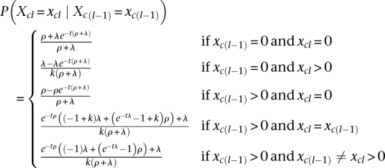 |
where t is the genetic distance between SNP locus l−1 and SNP locus l. The full transition probability, P(X.l = x.l | X.l−1 = x.l−1) for a given locus l, is simply calculated as the product of the transition probabilities for the individual chromosomes. The parameters λ and ρ will be inferred from the data. Because inferences will be done in a Bayesian framework, we must define a prior distribution for λ and ρ, P(λ,ρ). Uniform priors have been chosen in all applications in this study, but other priors could have been chosen.
Given the described emission and transition probabilities, the new model is quite standard for HMMs. It is described in detail in the Supplemental Material, section S1. Supplemental Material, section S1 also provides the mathematical derivation of an algorithm that allows us to calculate P(H,X | λ,ρ), the joint probability of the data and the IBD configuration.
It is important to note that the simplifying assumption that the instantaneous rate of transition between different non-zero IBD states is zero only means that such transitions are not allowed to happen over infinitesimal distances along the chromosome. Since the distance between any two loci is bigger than infinitesimal, the model does indeed, despite the assumption, allow such transitions to happen between any two loci, as is evident from the fact that the transition probabilities indicated above for such transitions is non-zero when t > 0.
It is it also worth noting that the described model reduces to the inbreeding model by Leutenegger et al. (2003) with a set to λ + ρ and f set to 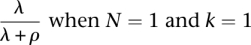 . This is noteworthy both because it illustrates that the new model can be viewed as an extension of the model by Leutenegger et al. (2003) and because the reparameterization to a and f contributes some additional intuition about the parameters λ and ρ. As in the model by Leutenegger et al. (2003), a (= λ + ρ) determines the overall instantaneous rate of change between IBD and non-IBD states and
  is the stationary probability of a non-zero IBD state.
Using this new model, we wish to estimate P(X, λ, ρ|H), the joint posterior distribution of the parameters of the model and the IBD configuration for each site. To do so we construct an MCMC method. MCMC methods are simulation methods that now are commonly used in genetics and genomics for estimating posterior distributions using simulations. These algorithms work by first initializing the parameters to some values and then repeatedly proposing changes to the parameter values using some stochastic algorithm. The parameter changes are accepted with a certain probability that depends on the likelihood calculated under the current and the proposed parameter values. The values of the parameters in the simulations then form a Markov chain, and standard Markov chain theory guarantees that if the simulation algorithm is repeated for a sufficiently long time, parameter values sampled from the simulations follow the desired posterior distribution and can be used to represent this distribution. The algorithm used in our case is described in the Supplemental Material, sections S2 and S3. This algorithm proposes changes from (λcur, ρcur, Xcur) to (λprop, ρprop, Xprop) with probability q(λcur, ρcur, Xcur → λprop, ρprop, Xprop). These proposed changes are then accepted with probability
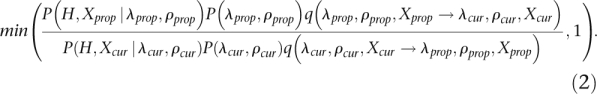 |
The values of X sampled from these Markov chain simulations then provide an estimate of the posterior distribution of X, and directly provide various forms of IBD probabilities between pairs of sequences and between larger sets of sequences. For example, for the BRCA1 data set consisting of SNP data from five cancer patients, later analyzed, the posterior probability that all five patients share the BRCA1 gene IBD can simply be approximated by the fraction of MCMC samples in which these five patients all share the BRCA1 gene IBD. Similarly, the posterior expectation of the number of these patients that share at least one chromosome IBD in the BRCA1 gene can be approximated by the mean number of the patients that share this gene IBD in the MCMC samples.
The Supplemental Material, sections S1, S2, and S3, provides all details of both the HMM and the MCMC algorithm. It also describes the method we use for incorporating genotyping errors and unknown phasing of the genotype data.
Simulated test data
To test the performance of the MCMC method and to compare it with existing methods we simulated data sets for a number of different conditions by
Specifying an IBD scenario (number of individuals N, number of SNP loci L, distances between loci and the IBD set partitioning of the 2N chromosomes for each locus).
Sampling a minor allele frequency (MAF) uniformly between 0.05 and 0.5 for each locus to mimic the high frequencies observed in data from most genotyping platforms.
Making a haplotype data set for each locus, by independently sampling an allele (A or a) for each IBD set in the locus based on the MAF of the locus, and then assigning an allele to each of the 2N chromosomes according to the IBD sets they belong to.
Adding errors at rate r.
Collapsing the two haplotypes for each individual into genotypes to achieve unphased data.
Estimating population allele frequencies based on sampling a number of extra individuals (subsequently used as input for the MCMC method instead of the “real” allele frequencies).
For the first IBD scenario we used 10 individuals, 501 equidistant SNPs covering a region of 8 Mb, an error rate of 0, and 10,000 extra individuals for estimating population allele frequencies. For the rest of the scenarios we used four individuals, 201 equidistant SNPs also covering a region of 8 Mb, an error rate of 0.003 to mimic realistic SNP chip error rates, and 100 extra individuals for estimating population allele frequencies corresponding by and large to a HapMap population sample size. The latter scenarios are thus both more realistic and more challenging than the first one.
All of the IBD scenarios used are described thoroughly in the Results section. Note that for the MCMC analyses, the extra individuals were not included in the IBD analysis; they were only used to get better estimates of population allele frequencies. Likewise, they were not included in the actual IBD analyses for any of the other methods we tested. However, for fairness we, of course, made the extra individuals available for all the methods to improve estimation of allele frequencies and other similar population-specific information. Hence, for instance, the method BEAGLE (Browning and Browning 2010) was allowed to use them for estimating haplotype clusters prior to IBD estimation.
We used a recombination rate of 1.3 cM per 1 Mb as estimated by Kong et al. (2002).
Power analysis
To evaluate the power and accuracy of the MCMC method, we used simulated data to compare it with four other methods; the method by Albrechtsen et al. (2009) implemented in the program Relate (version 0.994), the method by Purcell et al. (2007) implemented in the program PLINK (version 1.07), the method by Browning and Browning (2010) implemented in the program BEAGLE (version 3.3.0), and the method by Gusev et al. (2009) implemented in the program GERMLINE (version 1.3). When comparing to GERMLINE we used the option that allows for inference from unphased data.
We note that the four methods are all pairwise methods that cannot directly evaluate IBD relationships among more than two individuals. As such, the goal of our method is much more ambitious than any previous method for seemingly unrelated individuals, in that it allows analyses of IBD relationships among multiple individuals. However, our simulation study only allows comparison among the methods in the efficacy to determine pairwise IBD relationships.
We performed the comparison by first simulating data for six different IBD scenarios, each consisting of an IBD sharing pattern for four individuals in an 8-Mb region (see section “Simulated Test Data and Results” for details about the simulation method and the scenarios, respectively). For each scenario, we simulated 500 positive data sets with the scenario-specific IBD sharing pattern and 500 corresponding null data sets, with the exact same IBD sharing patterns, except that for scenario 1 the IBD sharing between the two chromosomes of individual 1 is removed and for the rest of the scenarios the IBD sharing between individuals 1 and 2 is removed. We then applied the MCMC method, Relate, PLINK, BEAGLE, and GERMLINE to all 6000 data sets. And finally, based on the results, we compared the methods. For scenario 1 the methods were compared on their ability to find the region of IBD sharing within individual 1, and for the rest of the scenarios the methods were compared on their ability to find the region of IBD sharing between individuals 1 and 2. The comparison was performed by producing ROC curves and by calculating the power of the different methods at significance levels 0 and 0.05. For all of the methods, except for GERMLINE, the ROC curves were produced as follows: We defined a region to be inferred as IBD when at least frac = 95% of the SNPs in it have a posterior probability higher than a given threshold t. For each scenario, any given threshold value t thereby determines a true-positive (TP) rate, namely, the fraction of positive sets for which the IBD sharing region of interest is (truly) inferred, and a false-positive (FP) rate, namely, the fraction of null sets in which the same region is (falsely) inferred to be IBD. The ROC plots were produced by plotting (FP rate, TP rate) for a number of thresholds. For GERMLINE, the ROC curves were produced in a similar manner. However, since GERMLINE, as opposed to all the other methods, does not output probabilities of IBD sharing, but instead outputs a list of inferred IBD regions, the thresholds used were instead the lower limits on the length of a potential IBD that were used when running GERMLINE.
For all five methods, the power values at significance level 0 and 0.05 were found by taking the TP rate corresponding to a FP rate of 0 and 0.05, respectively. In some cases, a FP rate of 0.05 was not observed. For theses cases, we instead indicate power as an interval with the TP rate that corresponds to the FP rate closest to 0.05 on each side as end points.
The process of producing ROC curves and power values was repeated with frac = 50 and frac = 100 to ensure that the choice of frac was not a determining factor for the conclusions we make based on the power study. For details on how the different programs were applied, see Supplemental Material, section S5.
Real test data
To test the applicability of the method to real data, we applied it to two human data sets. The first data set consists of five patients with breast and/or ovarian cancer, four Danes and one Greenlandic Inuit. These individuals are all heterozygous for a recently identified mutation in their BRCA1 gene on chromosome 17 (Hansen et al. 2010). Except for two of the individuals that have a coancestry coefficient of 0.107, the individuals are seemingly unrelated (the remaining coancestry coefficients are all lower than 0.014).
The second data set was the Center d'Etude du Polymorphisme Humain (CEPH) population from HapMap phase II (Frazer et al. 2007). It consists of 30 trios of European ancestry. However, we excluded the offspring, leaving us with 60 seemingly unrelated individuals. This second data set was included for two purposes. The main purpose was to improve all estimates of population genetic parameters, such as allele frequencies and LD that is needed prior to the IBD analysis of the first data set. Hence, the main purpose was to play the same role as the “extra individuals” did in the simulated data. The second purpose was to serve as controls in the disease mapping. For the latter, 10 randomly sampled individuals were included in the IBD analysis together with the five individuals from the first data set.
We emphasize that in real disease mapping studies it is advisable to have better matched controls or otherwise to control for population structure.
Both data sets were genotyped using the Affymetrix Sty chip which contains ∼225,000 SNPs. The base calling was performed using the BRLMM algorithm (Affymetrix 2006). The first data set was genotyped and called by Hansen et al. (2010), the second by Affymetrix.
Before applying the MCMC method, we pruned away a number of SNPs. First, we removed all SNPs that were not from chromosome 17. Then, we removed all SNPs with missing data and all SNPs with a minor allele frequency below 0.05. Finally, we removed LD by removing SNPs with an r2 value above 0.2 and a LOD score above 2 in a sliding window of 100 SNPs using a step size of 1. This left us with 1278 SNPs.
For genetic distance we used the positions supplied by HapMap (Frazer et al. 2007).
Calculation of Bayes Factors
As a part of the analysis of disease-related mutations, we calculated Bayes Factors in order to test different hypotheses (see the Results section for details about the specific hypotheses). A Bayes factor summarizes how much our relative belief in the hypothesis has increased by the information in the data compared with our belief in the hypothesis before observing the data.
To calculate a Bayes Factor (BF) for hypothesis (or model) M1 over hypothesis (or model) M2, we used the following formula:
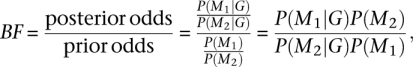 |
where G is the observed unphased genotype data. Both the posterior and the prior probabilities were estimated using the MCMC method. The prior probabilities were estimated by running the MCMC method with the likelihood of the data set to a constant value. We estimated the priors, because it is difficult to find analytical expressions for them. MCMC estimation of the priors on the other hand is straightforward to perform for any hypothesis.
Relatedness mapping
For relatedness (IBD) mapping we used two different statistics. The first statistic, stat1, is the posterior expected number of cases that share at least one chromosome IBD with another case. The second statistic, stat2, is the posterior probability of all cases sharing at least one allele IBD. The mapping was performed by running the MCMC method on five cases plus 10 additional individuals from the HapMap CEPH population as controls. We then calculated the test statistics for each locus for the five real cases. Finally, we obtained critical values for the test statistics by permuting the case-control labels. More precisely, for each of the two statistics we obtained experiment-wide critical values from the distribution among permutation replicates of the maximum of the test statistic over all loci, thereby controlling for multiple testing.
Results
An example run
We first made an initial test to ensure that the method is mathematically correct and correctly implemented. A description of this test and the test results can be seen in the Supplemental Material, section S5. The test was successful.
We then turned our attention to evaluating the efficacy of the method for solving IBD inference problems. To do so, we first applied the method to an example data set consisting of simulated unphased genotype data set for 10 individuals in a 8-Mb region containing 501 equidistant SNPs without LD between them (see Methods for details about the simulation approach). No errors were added when simulating the data, and allele frequencies were estimated from a very large population sample. The genotype data was simulated based on the IBD configuration in Figure 1A. This configuration contains several long and several short regions of IBD sharing between non-inbred individuals, an inbred individual, and IBD sharing between an inbred individual and a non-inbred individual. This simulated data set contains a broad range of the IBD sharing patterns that can be encountered in real data, thus applying the MCMC method to it should give a good overall idea of how well the method works for IBD inference. We ran the MCMC method with two different starting values in order to be able to properly assess if convergence had been reached. If the MCMC has been run for a too short amount of time, the samples obtained from the simulations will not reflect the correct distribution. To address this problem it is common practice to run multiple replicate simulations of the Markov chain and compare the results. Various statistics can then be used to assess if the simulations were run for a sufficiently long amount of time, i.e., if the chains have converged. The statistic we use is the Gelman-Rubin statistic (Gelman and Rubin 1992; Brooks and Gelman 1997), called the “potential scale reduction factor.” When the value of this statistic is close to 1, it is assumed that the simulations have converged. As can be seen in the Gelman-Rubin plot in Figure 2 the potential scale-reduction factor stabilizes at a value close to 1 after a few thousand iterations. This suggests that the chains did indeed reach convergence. For more information about convergence assessment of all other runs of the MCMC method presented in this study, see the Supplemental Material, section S6.
Figure 2.

Gelman-Rubin plot based on the number of zeros in the sampled IBD configurations. The MAP estimates that the inference it was based on is only a summary statistic in the sense that it summarizes all samples in one overall statistic per locus and not a statistic for each sample. Hence, it cannot be used for convergence monitoring. Instead, we used the number of zeros in the IBD configuration since this, at least to some extent, captures the state of the entire IBD configuration. The solid line is the Gelman-Rubin “potential scale reduction factor” and the dashed line is the upper 95% confidence limit of the “potential scale reduction factor.”
The inferred IBD configuration can be seen in Figure 1B. This inferred configuration is simply the IBD set partitioning with the highest posterior probability, i.e., maximum a posteriori (MAP) estimate, for each locus. As intended, the method can, at least in this example, very accurately infer both inbreeding and IBD among multiple individuals in the presence and absence of inbreeding. Also, and most importantly, the method is able to detect very short IBD regions of length <1 Mb.
The MCMC method is constructed such that transitions directly between different IBD sets are not allowed. Therefore, it is perhaps surprising that the inferences on data such as the data in Figure 1, where direct transitions between different IBD sets do occur, are so accurate. The simplifying assumption of no direct transitions between different IBD sets seems not to affect the accuracy of the method much, even when such transitions exist.
For comparison we ran four of the main competing methods, Relate, PLINK, BEAGLE and GERMLINE, with default settings on all the pairs of individuals. Except for GERMLINE, they all found all the long IBD regions that are shared between individuals. BEAGLE also found the long region of IBD sharing within individual 6 (BEAGLE is the only one of the four software packages that offers inbreeding inference). However, none of the four methods found any of the short (<1Mb) regions that are shared between the individuals.
Power analyses
Of course, nothing can be concluded from the above example run alone. Therefore, to quantify to what extent the above observations are true in general, we simulated 1000 data sets for each of six simple IBD scenarios. The simulated data sets all consist of genotype data for four individuals from an 8-Mb region containing 201 equidistant SNPs loci without LD between them. The IBD configurations underlying the six scenarios are illustrated in Figure 3.
Figure 3.

The IBD scenarios used in the power analysis. For each of the scenarios there is one colored line for each of the eight chromosome sequences. In addition, each column represents a locus in the data set. If a chromosome sequence in a given locus is green it means that it is shared IBD with all the other chromosome sequences of this color in that locus. If it is gray, it means that it is not IBD with any of the other chromosomes.
The scenarios are meant to represent the most important IBD patterns in the previous IBD configuration: (1) IBD within an individual, i.e., inbreeding, (2) long regions of IBD sharing between two non-inbred individuals, (3) long regions of IBD sharing between two individuals in the presence of inbreeding, and (4) very short regions of IBD sharing between non-inbred individuals. The latter is represented by three scenarios: (4a) short regions of IBD sharing supported by longer IBD sharing regions in other individuals, (4b) short IBD sharing regions, supported by a lot of IBD sharing in the area, and (4c) a short IBD sharing region with no support from IBD sharing between other individuals. Scenarios 4a and 4b are examples of situations where simultaneous analysis of all individuals, in theory, should increase power. Scenario 4c is an example of the opposite, and is included to test if the MCMC method in practice gains power from simultaneous analysis of multiple individuals.
We applied the MCMC method, Relate, PLINK, BEAGLE, and GERMLINE to the simulated data sets, and based on the results we assessed the power and accuracy of the methods for each of the six scenarios. More specifically, for scenario 1 we assessed the power and accuracy with which the methods were able to detect the region of IBD sharing within individual 1 and for the remaining five scenarios we assessed the power and accuracy with which the methods were able to detect the region of IBD sharing between individual 1 and individual 2. For instance, for scenario 3 the methods are assessed on their power and accuracy to detect that individual 1 and individual 2 share at least one chromosome IBD from locus 1 to locus 100. The reason why we only focus on the IBD sharing between individual 1 and 2 (and within individual 1) and not the entire IBD configuration is that Relate, PLINK, BEAGLE, and GERMLINE are all pairwise methods. Hence, in order to make a comparison possible we had to limit the test to pairwise IBD inference.
For details about the simulation approach and about how power calculations were performed, see Methods, and for details about how the programs were applied see the Supplemental Material, section S5. What should be noted here is that for this test, PLINK and GERMLINE were not run with default parameter values, as this resulted in extremely poor results. For instance, PLINK only managed to infer 0.3% of the IBD regions in scenarios 4a, 4b, and 4c.
The power at false-positive rates (FP rates) 0 and 0.05 of each of the five methods in the six scenarios is shown in Table 1, A and B, respectively. A subset of the ROC curves that these power calculations are based on are shown in Figure 4. The remaining ROC curves are shown in the Supplemental Material, section S7.
Table 1.
Power values

Figure 4.

ROC curves for the six scenarios. The definition used for calling an IBD region inferred for these curves is when at least 95% of the SNPs in the region are inferred to be IBD. The green points are from the MCMC method, the purple points are from Relate, the blue points are from PLINK, the red points are from BEAGLE, and the black points are from GERMLINE. The green and blue points are almost not visible in the plots for scenarios 2 and 3 because the purple points cover them. The red points are difficult to see in several of the plots, because in these plots the amount of unique points is very low. It should be noted that BEAGLE is based on a model that is highly dependent on the presence of LD, and therefore has the potential to perform much better than it does in this test if applied to data with LD.
Inspection of Table 1, A and B, shows that both the MCMC method and BEAGLE have full (100%) power to detect inbreeding, a feature the three other methods do not offer. The results also show that all five methods have full or at least high power to detect long IBD regions in the absence of inbreeding, even at a very low FP rate. However, and perhaps somewhat surprisingly, all methods also have full power to detect IBD between individual 1 and individual 2 in the presence of inbreeding in individual 1, even though Relate, PLINK, and BEAGLE are based on an explicit assumption that there is no inbreeding present. Thus, the results suggest that for long IBD regions, all five methods seem to perform well, and that specifically, the MCMC method seems to perform at least as well as the other methods.
For the scenarios with very short IBD regions the power analysis reveals that the MCMC method has considerably more power to detect short IBD regions than Relate, PLINK, BEAGLE, and GERMLINE. This is especially true in scenarios where simultaneous inference from multiple individuals provides a distinct advantage. As seen from the ROC curves for the MCMC method in scenarios 4a, 4b, and 4c in Figure 5, it is clear that the method indeed does achieve higher power when there is additional information to obtain from simultaneous analyses (scenarios 4a and 4b). However, the MCMC method actually also has higher power than the other methods in scenario 4c, where there is no extra information to achieve by analyzing the individuals simultaneously. We believe that this, at least in part, is due to the fact that the MCMC method takes the uncertainty of λ and ρ into account by allowing these to be parameters estimated from the data during the MCMC procedure. For comparison, the results from PLINK and Relate are achieved by first finding point estimates for the equivalent parameters and then using these as the ”true” parameter values in the subsequent analyses. The results from BEAGLE are achieved using user supplied values as ”true” values of the equivalent parameters.
Figure 5.

ROC curves for scenarios 4a, 4b, and 4c using the MCMC method. The curves for scenario 4a (dark green), 4b (light green), and 4c (yellow) were all calculated with an inference criterion of 95% SNPs detected.
Overall, the new MCMC method seems to have considerably more power to detect IBD sharing in data without LD than the four other methods. In fairness, it should be noted that Relate, BEAGLE, and GERMLINE are all able to handle data with LD, which the MCMC method is not. In fact, BEAGLE is based on a model that is highly dependent on the presence of LD, and therefore has potential to perform much better than it does in this test if applied to data with LD. Also, it should be noted that the gain in power comes at a price: the runtime of the MCMC method is significantly longer. Whereas the mean runtime for each of the above scenarios is a little less than 18 min for the MCMC method, the runtime of the other methods is on the order of seconds. A complete list of runtimes for all of the runs of the MCMC method presented in this study can be seen in Table 2.
Table 2.
Summary information for all MCMC analyses in this study

Applications to analyses of disease-related mutations
To illustrate the potential of the MCMC method for analyses of disease-related questions, we applied it to SNP chip data from a recent study by Hansen et al. (2010). In this study a disease-causing point mutation in the BRCA1 gene was identified in a Greenlandic Inuit with ovarian cancer (Hansen et al. 2010). It was the first report of this specific point mutation in the Greenlandic Inuit population, but the same point mutation had previously been observed among four Danes with breast and/or ovarian cancer. By use of pairwise IBD analysis with Relate, Hansen et al. (2010) investigated whether or not all five cancer patients share the allele IBD and found it very likely that they do, and thus, that their mutations are all caused by a single founder mutation. As a consequence, the authors recommended that the current approach to genetic screening of Greenlandic Inuit families with breast and/or ovarian cancer should be changed.
This study is a recent example of how questions regarding IBD sharing in a specific region can have important medical implications. It also illustrates the utility of the MCMC method as a tool for answering such questions in a probabilistic manner.
We applied the MCMC method to SNP data from a 12-Mb region surrounding the BRCA1 gene, and to compare with the pairwise methods, we also applied Relate, PLINK, BEAGLE, and GERMLINE to the same data. The first three of these methods were applied with essentially the same settings as in the power study, and GERMLINE was run with default values (see the Supplemental Material, section S4, for details about the program settings used). All five methods were applied to the data with the purpose of answering the question posed in the original study: do all five individuals share the disease-causing mutation IBD?
The pairwise results for all of the five methods can be seen in Figure 6. Here, the probability that each of the 10 pairs of individuals share at least one chromosome IBD in the BRCA1 gene is plotted (since GERMLINE does not provide probabilities, we simply set the probability to 1 if the individuals were inferred to be IBD and 0 if they were not).
Figure 6.

Probabilities of sharing at least one chromosome IBD between all 10 pairs of affected individuals in the BRCA1 gene. The probabilities are depicted for the MCMC method, Relate, PLINK, BEAGLE, and GERMLINE, respectively.
As can be seen, the five methods give very different pairwise results. The MCMC method infers that there is a high probability that all of the pairs are IBD in the BRCA1 region. Relate infers that there is a high probability of IBD sharing between almost all pairs of individuals, with the exception that “Dane1” only seems to be IBD with the Greenlandic Inuit (exactly as reported by Hansen et al. 2010). PLINK gives the same overall picture as Relate, except that PLINK only infers “Dane1” to have an intermediate probability of sharing the BRCA1 region IBD with the Greenlandic Inuit. BEAGLE also gives the same overall picture as Relate, except that BEAGLE infers very low IBD sharing probabilities between “Dane1” and “Inuit” and between “Dane2 and “Dane4” and it only infers an intermediate probability of IBD sharing between “Dane2” and “Dane3”. Finally, GERMLINE only infers IBD sharing between two of the individuals.
There are three important differences between the answers that the five methods provide. First, and most importantly, due to their pairwise nature, the pairwise methods only provide pairwise probabilities like the ones shown in Figure 6. The pairs are correlated, and it is unclear how the pairwise probabilities should be combined into one overall probability. Therefore, questions about more than two individuals like the one posed here cannot be addressed directly in a strict probabilistic manner. Having only pairwise methods available Hansen et al. (2010) were only able to answer the question indirectly. Using pairwise probabilities and a plot of the average IBD sharing probabilities, Hansen et al. (2010) argued that it is very likely that they all share the region IBD. The MCMC method on the other hand, answers this question directly. By calculating the fraction of the samples in which all five individuals are IBD in the BRCA1 region, we can estimate the posterior probability that all five individuals share this region IBD to be 0.67. Using the MCMC method we can also easily provide a Bayes Factor for the hypothesis that all of the individuals share their BRCA1 region IBD versus the hypothesis that they do not all share the region IBD. In this case it is ≃97, which means that there is very strong support for the hypothesis that they all share their BRCA1 region IBD, and thus, that the disease-causing mutation is a founder mutation.
Second, the results from the pairwise methods are not always consistent. For instance, the Relate results are somewhat odd. They can only be correct if the Greenlandic Inuit shares one allele IBD with “Dane1” and the other allele IBD with the rest of the Danes, which is very unlikely. Hence, it seems that Relate is either incorrectly inferring IBD sharing between the Greenlandic Inuit and “Dane1” or that it does not have enough power to detect IBD sharing between “Dane1” and the other individuals. If the former is true, it would lead us to conclude that only four of the individuals share the disease-causing mutation IBD. If the latter is the case, all five individuals share the mutation IBD. Such ambiguous results make it difficult to answer questions about IBD relationships among multiple individuals indirectly using pairwise methods, because these methods do not provide any obvious approach for testing different hypotheses statistically. The MCMC method, on the other hand, always provides consistent results. Moreover, if two hypotheses both seem probable, the MCMC method facilitates statistical discrimination between hypotheses. For instance, it allows us to calculate a Bayes Factor for the hypothesis that all of the individuals share their BRCA1 gene IBD versus the hypothesis that only Danes 2, 3, and 4 and the Greenlandic Inuit share the region IBD. Based on the previously published Relate output, this would be an important question to address. This Bayes Factor is ≃9; thus, there is substantial support for the hypothesis that they all share the region IBD.
Third, and last, the pairwise methods clearly give very different results. In general, the pairwise methods infer less IBD pairwise sharing than the MCMC method. To be as fair as possible to Relate, BEAGLE, and GERMLINE, we only removed SNPs in LD from the data used by PLINK and the MCMC method, since Relate, BEAGLE, and GERMLINE can analyze SNPs in LD and can thus potentially benefit from the extra genotype information. This difference in input data is, of course, one possible explanation that these methods infer less IBD than the MCMC method. However, including SNPs in LD did not cause either Relate, BEAGLE, or GERMLINE to infer less IBD. On the contrary, running Relate, BEAGLE, and GERMLINE on the LD reduced data set results in the same or lower IBD sharing probabilities for almost all pairs (up to 0.4 lower). In addition, in the few cases where this is not the case, the IBD probability only becomes slightly higher (<0.1). This is most likely because the LD free data set have fewer SNPs and, therefore, contain less information. Another possible explanation for the different results is that all five individuals actually do share the mutation IBD, but that some of the shared regions are too short for Relate, PLINK, BEAGLE, and GERMLINE to accurately infer them. We find this explanation very plausible. It appears very likely that the reason that GERMLINE finds much fewer IBD regions than the other methods is that it (per default) has very strict requirements for detecting IBD regions at this scale. If we relax the default settings as we did in the power simulations, we find that the more we reduce the lower bound on IBD regions length, the more putative IBD regions are inferred. Indeed, if we set it low enough, all pairs are inferred to be IBD in the BRCA1 region. However, as it is unclear which settings to use (in order to avoid a vast amount of false positives), we used the default settings.
As already reported in Hansen et al. (2010) some of the IBD regions that are inferred by Relate are rather short (down to 1–2 Mb). MAP estimates based on output from the MCMC method also suggest that some of the IBD regions containing the BRCA1 gene are relatively short (see Supplemental Material: Supplemental Fig. S13). This, combined with the fact that the results from Relate, and to some extent PLINK and BEAGLE, seem internally inconsistent, makes it seem likely that Relate, PLINK, and BEAGLE infer fewer IBD regions than the MCMC method, due to lack of statistical power, since Relate, PLINK, and BEAGLE do not take information about more than two individuals into account at a time. In fact, this explanation was proposed by Hansen et al. (2010). Hence, it appears that the increased power of the MCMC method is not only of theoretical interest, but also results in tangible improvements when it is applied to real data.
Overall, these observations suggest that the MCMC method constitutes a very good alternative to the pairwise methods for inferring IBD relationships in a probabilistically sound manner in cases where the computational demands of the method are not prohibitive.
Applications to disease mapping
We further illustrate the potential of the method for IBD-based disease gene mapping by applying it to the data set discussed above: a set of five cancer-affected individuals with the same disease-causing mutation in the BRCA1 gene on chromosome 17. We applied the MCMC method to all of chromosome 17 of the five cases and 10 additional controls (HapMap individuals) and performed a test for increased IBD sharing among the cases by permutation of the case/control labels of the individuals. In real disease mapping studies, we would encourage the use of better-matched controls and/or the use of a statistical correction for population structure. We used two different mapping statistics for the test: stat1, which is the posterior expected number of cases that share at least one chromosome IBD with another case, and stat2, which is a simple indicator of whether or not all cases share at least one allele IBD. Other statistics might be more appropriate in other cases depending on the underlying inheritance model and on the number of founder mutations/defective alleles that cause the disease. The P-values corresponding to each of the two chosen statistics along chromosome 17 can be seen in Figure 7. The depicted P-values have been corrected for multiple testing in the permutation procedure. As can be seen, stat1 allows us to identify a 9.2-Mb region (using a significance level of 0.01), and stat2 allows us to identify a 7.6-Mb region (again using a P-value cut-off of 0.01), both containing the BRCA1 mutation. It is worth noting that if we use an even stricter significance level (0.0005) stat2 actually allows us to narrow the region down to a size of only 2.2 Mb still containing the BRCA1 gene. Hence, based on very simple statistics and data from only five affected individuals we are actually able to map the region with the disease-causing mutation down to a very small region. In contrast to family-based IBD mapping, relatedness mapping (IBD mapping based on population data) allows the identification of a very small genomic region containing the causal variant, i.e., it has increased mapping accuracy. The reason is that relatedness mapping gains information from all the meiosis in the pedigree relating the individuals carrying the founder mutation.
Figure 7.

P-values based on two different statistics, stat1 and stat2. (A) P-values based on stat1, which is the posterior expected number of cases that share at least one chromosome IBD in each locus. (B) P-values based on stat2, which is a simple indicator of whether or not all cases share at least one allele IBD. All P-values are corrected for multiple testing.
In the example shown here, the five individuals were chosen because they share a single mutation. For relatively common diseases, such as breast and ovarian cancer affected by the BRCA1 locus discussed here, analyses of five individuals are unlikely to be very helpful in practice because of genetic heterogeneity. It is unlikely that all individuals will share the same mutation and larger samples will typically be needed. A full exploration of the relationship between statistical power, degree of allelic heterogeneity, and penetrance is not the objective of this study, but see Albrechtsen et al. (2009) for more discussion regarding power in studies based on relatedness mapping.
Discussion
We have presented a new method for identifying regions that two or more chromosomes share IBD using nothing but unphased SNP data. In contrast to the current competing methods, which all are pairwise methods, our method models IBD sharing among multiple individuals simultaneously while taking parameter uncertainty into account. We have shown that this leads to higher power for finding short IBD regions, even in pairwise comparisons. We have also shown that our approach can answer a broad range of medically relevant questions in a probabilistic manner, which cannot be answered directly by other methods. Finally, we have provided an example of an application to real data; we have shown that the method can be used for quite accurate disease mapping using only unphased SNP data from five affected individuals. Neither association mapping nor linkage mapping could have detected associations from these data. Linkage mapping could not be applied because the pedigree relating the five individuals is not known. Genome-wide association mapping would essentially have zero statistical power, because the data set is too small (five cases). Of course, this does not mean that the new method should entirely replace linkage mapping or association mapping. The method will only have significant power if the mutation(s) is so rare/recent that IBD regions around the mutation can be inferred. In addition, the size of the region inferred to contain the causal mutation(s) might be large if the number of meiosis in the (unobserved) pedigree relating the individuals is small. However, when a disease is caused by one or a few rare founder mutations, the MCMC method provides a good alternative to the standard approaches, in the sense that mapping can be done with reasonable resolution using only unphased SNP chip data from very few seemingly unrelated individuals.
An important drawback of the method presented is, however, that it is significantly slower than all other current methods for detecting IBD as shown in Table 2. The method cannot be applied directly to whole genomes for hundreds or thousands of individuals. For this purpose, programs like Relate, PLINK, BEAGLE, and GERMLINE are much better suited, as least for the initial analysis. Subsequent analyses of candidate regions can then be carried out using the MCMC method. The MCMC method can also be used on a whole chromosome—and thus genome-wide—for a limited number of individuals. A second important drawback of the MCMC method in comparison to Relate and BEAGLE is that it does not take LD into account. Unfortunately, it is not trivial to correct for LD in the multi-individual case on unphased data. For data sets where it is important to take LD into account, one could, however, implement the method for phased data. In this case, it is fairly straightforward to use the same principle for LD correction as used in Relate. This would potentially also make the method significantly faster. Hence, it might be a good future approach for dealing with larger data sets, especially as algorithms for phasing improves.
However, even taking these drawbacks into account, the new method provides a substantially novel approach for analyzing genetic data, and a new accurate method for identifying rare disease-causing mutations. It should find applications, in particular for the mapping of rare diseases, for which only few cases can be obtained, but in which one or a few mutations are causing the disease. It might provide a strong alternative to genome-wide association mapping for populations with small effective population sizes, such as the Greenlandic Inuit population.
Acknowledgments
This research was supported by The Danish Council for Independent Research | Medical Sciences (FSS), the NEYE Foundation, NIH grants NIGMS R01-HG003229–05 and R01-HG003229–0551, and the American Recovery and Reinvestment Act of 2009.
Footnotes
[Supplemental material is available for this article. The MCMC software is freely available at http://people.binf.ku.dk/ida/Software/MCMC_IBDfinder/.]
Article published online before print. Article, supplemental material, and publication date are at http://www.genome.org/cgi/doi/10.1101/gr.115360.110.
References
- Abecasis GR, Cherny SS, Cookson WO, Cardon LR 2002. Merlin–rapid analysis of dense genetic maps using sparse gene flow trees. Nat Genet 30: 97–101 [DOI] [PubMed] [Google Scholar]
- Affymetrix Inc. 2006. Brlmm: an improved genotype calling method for the genechip human mapping 500k array set. http://www.affymetrix.com/support/technical/whitepapers/brlmm_whitepaper.pdf.
- Albrechtsen A, Korneliussen TS, Moltke I, Hansen TvO, Nielsen FC, Nielsen R 2009. Relatedness mapping and tracts of relatedness for genome-wide data in the presence of linkage disequilibrium. Genet Epidemiol 33: 266–274 [DOI] [PubMed] [Google Scholar]
- Albrechtsen A, Moltke I, Nielsen R 2010. Natural selection and the distribution of Identity By Descent in the human genome. Genetics 186: 295–308 [DOI] [PMC free article] [PubMed] [Google Scholar]
- Brooks SP, Gelman A 1997. General methods for monitoring convergence of iterative simulations. J Comput Graph Statist 7: 434–455 [Google Scholar]
- Browning SR 2008. Estimation of pairwise identity by descent from dense genetic marker data in a population sample of haplotypes. Genetics 178: 2123–2132 [DOI] [PMC free article] [PubMed] [Google Scholar]
- Browning SR, Browning BL 2010. High-resolution detection of identity by descent in unrelated individuals. Am J Hum Genet 86: 526–539 [DOI] [PMC free article] [PubMed] [Google Scholar]
- Cannings C, Thompson EA, Skolnick MH 1978. Probability functions on complex pedigrees. Adv Appl Probab 10: 26–61 [Google Scholar]
- Elston RC, Stewart J 1971. A general model for the genetic analysis of pedigree data. Hum Hered 21: 523–542 [DOI] [PubMed] [Google Scholar]
- Evett IW, Weir BS 1998. Interpreting DNA evidence: Statistical genetics for forensics scientists. Sinauer Associates Inc, Sunderland, MA [Google Scholar]
- Frazer KA, Ballinger DG, Cox DR, Hinds DA, Stuve LL, Gibbs RA, Belmont JW, Boudreau A, Hardenbol P, Leal SM, et al. 2007. A second generation human haplotype map of over 3.1 million SNPs. Nature 449: 851–861 [DOI] [PMC free article] [PubMed] [Google Scholar]
- Gelman A, Rubin DB 1992. Inference from iterative simulation using multiple sequences. Stat Sci 7: 457–511 [Google Scholar]
- Gusev A, Lowe JK, Stoffel M, Daly MJ, Altshuler D, Breslow JL, Friedman JM, Pe'er I 2009. Whole population, genome-wide mapping of hidden relatedness. Genome Res 19: 318–326 [DOI] [PMC free article] [PubMed] [Google Scholar]
- Hansen TV, Ejlertsen B, Albrechtsen A, Bergsten E, Bjerregaard P, Hansen T, Myrhj T, Nielsen PB, Timmermans-Wielenga V, Andersen MK, et al. 2009. A common Greenlandic Inuit BRCA1 RING domain founder mutation. Breast Cancer Res Treat 115: 69–76 [DOI] [PubMed] [Google Scholar]
- Hansen TV, Jønson L, Albrechtsen A, Steffensen AY, Bergsten E, Myrhøj T, Ejlertsen B, Nielsen FC 2010. Identification of a novel BRCA1 nucleotide 4803delCC/c.4684delCC mutation and a nucleotide 249T>A/c.130T>A (p.Cys44Ser) mutation in two Greenlandic Inuit families: implications for genetic screening of Greenlandic Inuit families with high risk for breast and/or ovarian cancer. Breast Cancer Res Treat 124: 259–264 [DOI] [PubMed] [Google Scholar]
- Hilden J 1970. GENEX An algebraic approach to pedigree probability calculus. Clin Genet 1: 319–348 [Google Scholar]
- Hirschhorn JN, Daly MJ 2005. Genome-wide association studies for common diseases and complex traits. Nat Rev Genet 6: 95–108 [DOI] [PubMed] [Google Scholar]
- Houwen RH, Baharloo S, Blankenship K, Raeymaekers P, Juyn J, Sandkuijl LA, Freimer NB 1994. Genome screening by searching for shared segments: mapping a gene for benign recurrent intrahepatic cholestasis. Nat Genet 8: 380–386 [DOI] [PubMed] [Google Scholar]
- Kong A, Gudbjartsson DF, Sainz J, Jonsdottir GM, Gudjonsson SA, Richardsson B, Sigurdardottir S, Barnard J, Hallbeck B, Masson G, et al. 2002. A high-resolution recombination map of the human genome. Nat Genet 31: 241–247 [DOI] [PubMed] [Google Scholar]
- Kruglyak L, Daly MJ, Reeve-Daly MP, Lander ES 1996. Parametric and nonparametric linkage analysis: a unified multipoint approach. Am J Hum Genet 58: 1347–1363 [PMC free article] [PubMed] [Google Scholar]
- Lander ES, Green P 1987. Construction of multilocus genetic linkage maps in humans. Proc Natl Acad Sci 84: 2363–2367 [DOI] [PMC free article] [PubMed] [Google Scholar]
- Leibon G, Rockmore DN, Pollak MR 2008. A SNP streak model for the identification of genetic regions identical-by-descent. Stat Appl Genet Mol Biol 7: Article16. doi: 10.2202/1544-6115.1340 [DOI] [PMC free article] [PubMed] [Google Scholar]
- Leutenegger AL, Prum B, Génin E, Verny C, Lemainque A, Clerget-Darpoux F, Thompson EA 2003. Estimation of the inbreeding coefficient through use of genomic data. Am J Hum Genet 73: 516–523 [DOI] [PMC free article] [PubMed] [Google Scholar]
- Lynch M, Ritland K 1999. Estimation of pairwise relatedness with molecular markers. Genetics 152: 1753–1766 [DOI] [PMC free article] [PubMed] [Google Scholar]
- Malecot G 1946. La consaguinite dans une population limitee. C R Acad Sci Paris 222: 841–843 [Google Scholar]
- Malecot G 1948. Les mathematiques de l'heredite. Masson, Paris, France [Google Scholar]
- Ott J 1974. Estimation of the recombination fraction in human pedigrees: efficient computation of the likelihood for human linkage studies. Am J Hum Genet 26: 588–597 [PMC free article] [PubMed] [Google Scholar]
- Purcell S, Neale B, Todd-Brown K, Thomas L, Ferreira MA, Bender D, Maller J, Sklar P, de Bakker PI, Daly MJ, et al. 2007. PLINK: a tool set for whole-genome association and population-based linkage analyses. Am J Hum Genet 81: 559–575 [DOI] [PMC free article] [PubMed] [Google Scholar]
- Queller DC, Goodnight KF 1989. Estimating relatedness using molecular markers. Evolution 43: 258–275 [DOI] [PubMed] [Google Scholar]
- Rabiner LR 1989. A tutorial on hidden markov models and selected applications in speech recognition. Proc IEEE 77: 257–286 [Google Scholar]
- Ritland K 1996. Estimators for pairwise relatedness and individual inbreeding coefficients. Genet Res 67: 175–185 [Google Scholar]
- Te Meerman GJ, Van der Meulen MA 1997. Genomic sharing surrounding alleles identical by descent: effects of genetic drift and population growth. Genet Epidemiol 14: 1125–1130 [DOI] [PubMed] [Google Scholar]
- Te Meerman GJ, Van der Meulen MA, Sandkuijl LA 1995. Perspectives of identity by descent (IBD) mapping in founder populations. Clin Exp Allergy Suppl 225: 97–102 [DOI] [PubMed] [Google Scholar]
- Thomas A 2010. Assessment of SNP streak statistics using gene drop simulation with linkage disequilibrium. Genet Epidemiol 34: 119–124 [DOI] [PMC free article] [PubMed] [Google Scholar]
- Thomas A, Camp NJ, Farnham JM, Allen-Brady K, Cannon-Albright LA 2008. Shared genomic segment analysis. Mapping disease predisposition genes in extended pedigrees using SNP genotype assays. Ann Hum Genet 72: 279–287 [DOI] [PMC free article] [PubMed] [Google Scholar]
- Thompson EA 1975. The estimation of pairwise relationships. Ann Hum Genet 39: 173–188 [DOI] [PubMed] [Google Scholar]
- Thompson EA 2008. The IBD process along four chromosomes. Theor Popul Biol 73: 369–373 [DOI] [PMC free article] [PubMed] [Google Scholar]
- Van der Meulen MA, Te Meerman GJ 1997. Haplotype sharing analysis in affected individuals from nuclear families with at least one affected offspring. Genet Epidemiol 14: 915–919 [DOI] [PubMed] [Google Scholar]