

Abstract
Developing accurate, scalable algorithms to improve data quality is an important computational challenge associated with recent advances in high-throughput sequencing technology. In this study, a novel error-correction algorithm, called ECHO, is introduced for correcting base-call errors in short-reads, without the need of a reference genome. Unlike most previous methods, ECHO does not require the user to specify parameters of which optimal values are typically unknown a priori. ECHO automatically sets the parameters in the assumed model and estimates error characteristics specific to each sequencing run, while maintaining a running time that is within the range of practical use. ECHO is based on a probabilistic model and is able to assign a quality score to each corrected base. Furthermore, it explicitly models heterozygosity in diploid genomes and provides a reference-free method for detecting bases that originated from heterozygous sites. On both real and simulated data, ECHO is able to improve the accuracy of previous error-correction methods by several folds to an order of magnitude, depending on the sequence coverage depth and the position in the read. The improvement is most pronounced toward the end of the read, where previous methods become noticeably less effective. Using a whole-genome yeast data set, it is demonstrated here that ECHO is capable of coping with nonuniform coverage. Also, it is shown that using ECHO to perform error correction as a preprocessing step considerably facilitates de novo assembly, particularly in the case of low-to-moderate sequence coverage depth.
Over the past few years, next-generation sequencing (NGS) technologies have introduced a rapidly growing wave of information in biological sciences; see Metzker (2010) for a recent review of NGS platforms and their applications. Exploiting massive parallelization, NGS platforms generate high-throughput data at very low cost per base. An important computational challenge associated with this rapid technological advancement is to develop efficient algorithms to extract accurate sequence information. In comparison with traditional Sanger sequencing (Sanger et al. 1977), NGS data have shorter read lengths and higher error rates, and these characteristics create many challenges for computation, especially when a reference genome is not available. Reducing the error rate of base-calls and improving the accuracy of base-specific quality scores have important practical implications for assembly (Sundquist et al. 2007; Butler et al. 2008; Li et al. 2008; Medvedev and Brudno 2008; Zerbino and Birney 2008; Chaisson et al. 2009; Langmead et al. 2009; Simpson et al. 2009; Peng et al. 2010); polymorphism detection, especially rare ones (Brockman et al. 2008; Li et al. 2008); and downstream population genomics analysis of NGS data (Hellmann et al. 2008; Jiang et al. 2009).
To improve data quality, it is well recognized that development of accurate, scalable computational tools must parallel the rapid advancement in sequencing technology. There are two main approaches to addressing this challenge: (1) One approach is to develop improved image analysis and base-calling algorithms. This line of work has been pursued by several researchers in the past, including ourselves (for review, see Erlich et al. 2008; Rougemont et al. 2008; Kao et al. 2009; Kircher et al. 2009; Whiteford et al. 2009; Kao and Song 2011). Indeed, by using more sophisticated statistical methods, it has been demonstrated that it is possible to deliver significant improvements over the tools developed by the manufacturers of the sequencing platforms. (2) An alternative approach is to correct for potential errors after base-calling has been performed by leveraging on the fact that each position in the genome on average is sequenced multiple times. Several methods have been developed for this approach (e.g., see Gajer et al. 2004; Chaisson et al. 2009; Chin et al. 2009; Qu et al. 2009; Schröder et al. 2009; Shi et al. 2009; Wijaya et al. 2009; Salmela 2010; Yang et al. 2010).
The goal of the present study is to introduce a novel, efficient computational method for the latter approach. Our error-correction algorithm is called ECHO, and it has the following notable features, most of which are unique to our method:
Whereas previous reference-free error-correction algorithms (Chaisson et al. 2009; Schröder et al. 2009; Shi et al. 2009; Salmela 2010) typically rely on the user to specify some of the key parameters, of which optimal values are typically unknown a priori, ECHO automatically finds the optimal parameters and estimates error characteristics specific to each sequencing run.
ECHO is based on a probabilistic framework and can assign a quality score to each corrected base. Quality scores are useful and sometimes necessary in downstream analysis.
Previous reference-free error-correction algorithms (Chaisson et al. 2009; Schröder et al. 2009; Shi et al. 2009; Salmela 2010) for short-reads are based on k-mer or substring frequencies. ECHO instead relies on finding overlaps between reads. Despite being more computationally intensive, this approach retains more of the information contained in the reads without aggregating away potentially useful relationships. Although error correction based on read overlap has been tried previously with Sanger reads (Batzoglou et al. 2002), ECHO differs from previous works in that it is specialized for high-throughput short-reads.
ECHO explicitly models heterozygosity in diploid genomes and allows one to process diploid data in a novel way. Specifically, for each length-l haplotype (or short read) in the input data, ECHO can infer a likely length-l genotype sequence from which the haplotype may have originated, and position-specific quality scores can be assigned to each genotype. For each input short read, this approach provides a way, in the absence of a reference genome, to detect the bases that originated from heterozygous sites in the sequenced diploid genome and to infer the corresponding genotypes.
ECHO performs error correction by first finding overlaps between reads. This procedure requires not only computational considerations to handle the enormous number of reads typically generated by NGS platforms, but also requires an effective method to filter out false overlaps. ECHO achieves this by imposing a maximum error tolerance in the overlaps and a minimum overlap length. These stringent requirements typically filter out many of the potential false overlaps, provided that the genome is not repeat rich. However, the optimal error tolerance and overlap requirement are usually unknown a priori. Whereas previous error-correction algorithms require the user to specify the key parameters, which may greatly affect the performance of the algorithm, ECHO automatically determines the optimal values for the error tolerance and minimum overlap length by utilizing assumptions on the coverage distribution of the reads.
Once ECHO determines the relevant parameters and finds the overlaps between reads, it estimates the error characteristics of the data using an expectation-maximization (EM) procedure. Our statistical approach attempts to accurately model the error behavior of the sequencing platform. This is in contrast to other error-correction algorithms that typically use an error threshold or coverage cutoff, which may not be statistically motivated. Furthermore, in ECHO, error modeling is performed for each input data set to characterize more effectively the unique properties of different sequencing runs. Utilizing the read overlaps and the error characterization, ECHO performs error correction on the reads using a maximum a posteriori procedure. Because the sequencing behavior is modeled statistically, meaningful quality scores can be assigned to the bases of the corrected reads.
Repeats in the genome are challenging to handle since they may lead to false overlaps. In general, ECHO is less sensitive to repeats than are previous error-correction methods that rely on k-mer or substring frequencies. By retaining the relationships among reads more explicitly, rather than computing aggregate statistics on substring frequencies, ECHO is better able to handle repeat patterns in the genome. However, the obstacles imposed by repeat regions are still significant, and more sophisticated methods that incorporate additional information will be necessary to overcome these challenges adequately.
To test the performance of our algorithm, we consider real short-read data generated by Illumina's Genome Analyzer (GA) I and II, as well as synthetic short-read data simulated to mimic GA's error characteristics. For GA, most of the sequencing errors are miscall errors (as opposed to indels), with the property that the error rate generally increases toward the end of the read. We show that ECHO is able to improve the accuracy of previous error-correction methods by several folds to an order of magnitude, depending on the sequence coverage depth and the position in the read. In particular, provided that the sequence coverage depth is moderate to high (roughly, 15 or higher), ECHO remains effective throughout the entire read length, typically reducing the error rate at the end of the read from over 5% to under 1%.
ECHO can process relatively small genomes such as that of yeasts or fungi on a desktop computer. To demonstrate this point and to show that ECHO is capable of coping with nonuniform coverage that may arise in real data, we apply our method on a real whole-genome yeast data set.
In addition to the improvement in data quality, we also examine here the effects of error correction on de novo assembly. Assembly is particularly challenging when the sequence coverage depth is low to moderate, and it may benefit considerably from the improved data quality delivered by error correction. In this study, we show that performing error correction as a preprocessing step facilitates de novo assembly significantly.
A software implementation of the algorithm described in this work is publicly available at http://uc-echo.sourceforge.net under the Berkeley Software Distribution License.
Methods
In this section, we describe our error-correction algorithm ECHO, which is divided into two stages: (1) neighbor finding, and (2) maximum a posteriori error correction. Since we assume that the reference genome is not available, we first devise a clustering algorithm to find “neighboring” reads that presumably cover the same region of the genome. Upon finding the putative neighbors of each read, we then correct for sequencing errors by using a maximum a posteriori estimation procedure for each base of the read.
Neighbor finding
In a sequencing run with a moderate-to-high coverage depth, each position in the genome on average is sequenced multiple times. The basic idea behind error correction is to leverage on this redundant information. When there is a reference genome, identifying the reads that cover the same region can be done via “read mapping” (Li et al. 2008; Langmead et al. 2009; Li and Durbin 2010). However, in the absence of a reference genome, the task of identifying neighbors becomes more challenging. Below, we devise a neighbor-finding algorithm based on hashing, rather than an explicit search of all pairs of reads, which would be computationally prohibitive. The approach is similar to the one in Batzoglou et al. (2002) to find overlaps between reads. However, their method is geared toward Sanger reads, whereas ECHO is specialized for short-read data, which requires different computational considerations.
In a preprocessing step, we first augment the set of reads with their reverse complements. For a given keyword length k, we iterate through the reads and their complements, and create a hash table mapping each k-mer to the reads that contain it, along with the position in the read where the k-mer occurs. If a k-mer occurs multiple times in a read, for computational efficiency we record only the position that is closest to the beginning of the read; this choice is motivated by the fact that, for the Illumina platform, early cycles of a sequencing run generally have higher quality than do later cycles. (If the read is instead a reverse complement that was added in the preprocessing step, we keep the position that is closest to the end of the read, which would have higher quality than the beginning.) Assuming k to be a constant, this hashing stage requires expected O(Nl) time, where N is the number of input reads and l is the read length.
Once the hash table mapping k-mers to the reads is constructed, we consider more thorough alignments to construct an adjacency list connecting neighboring reads together. We run through the k-mers, and for each one, consider its associated set of reads. For every pair of reads, we do a simple alignment to assess the quality of the overlap between the two reads. Figure 1 illustrates how the two reads are aligned given a common k-mer. We use ε to denote the fraction of errors in the overlap, i.e.,
where m is the number of mismatches in the overlap and ω is the length of the overlap. The “score” of an overlap is defined as 1/ε, and it is used to select the best alignment from among several possible alignments between two reads. Further, we require that the overlap length be greater than the minimum overlap parameter ω* and that the fraction of errors in the overlap ε be less than ε*, the error tolerance:
ω ≥ ω*, the overlap length must be at least the minimum required overlap length ω*.
ε ≤ ε*, the fraction of mismatched bases is less than the error tolerance ε*.
Figure 1.

Illustration of the alignment of two reads by identifying a common k-mer in the overlap. The boxes labeled by K denote a common k-mer between the two reads. The symbol × denotes a sequencing error that would preclude a common k-mer from occurring in the immediate area. However, as long as the error rate is low enough and the overlap is sufficiently long, a common k-mer will exist with high probability.
The two threshold parameters ω* and ε* are selected automatically in ECHO, as described below in Parameter selection.
In practice, the best alignment for the overlap between two reads involves aligning together their common k-mer, since it already provides k matching bases. In this case the alignment is given immediately by the position of the k-mer itself. Using this method, an alignment between a pair of reads is found in O(1) time. When two reads share multiple common k-mers, the scoring method described above is used to select the best alignment, and only the best alignment is kept in the adjacency list. In the case of ties, the alignment with the greatest overlap length is chosen.
Looking only at common k-mers between reads is typically sufficient to find overlaps, because for a small enough k, the chance that two truly overlapping reads do not have any common k-mer in the overlap is small, provided that the sequencing error rate is low. Both reads only need an error-free stretch long enough to cover the k-mer in the overlapping region for the reads to have a common k-mer. Given a relatively low error rate, this occurs with high probability. A similar idea is also utilized in Rasmussen et al. (2005) and Jokinen and Ukkonen (1991). Although the current implementation does not allow for indels in the overlaps, it would be straightforward to generalize this alignment step to accommodate for indels at the expense of greater computational cost.
With Bmax denoting the maximum number of reads associated with a single k-mer (i.e., the size of the largest bin in the hash table) and  denoting the total number of k-mers, the neighbor finding stage requires
  time. Here, O(Nl) is the time required for the hashing stage, and
  is the time needed to process the reads associated with every k-mer, where counting the number of mismatches in an overlap takes O(l) time and there are at most
  pairs of reads to consider for each k-mer. There are times when the number of reads that contain a given k-mer is abnormally large, e.g., when the k-mer is a substring of a repetitive region or the coverage of the genome is highly nonuniform. In our algorithm, we put a cap on the k-mer bin size in the hash table, such that the reads associated with a k-mer with an extreme number of overlaps are not corrected. This approach allows us to avoid correcting reads that belong to highly repetitive regions, for which the assumptions on overlaps become more tenuous.
Parameter selection
In ECHO, three parameters are required for finding the overlaps between reads: k, the keyword length; ω*, the minimum overlap length; and ε*, the threshold on the fraction of allowed errors in an overlap. The keyword length k must be chosen to balance two effects:
If k is too small, the number of reads associated with each k-mer will be very large. This exacerbates the running time during the neighbor-finding stage because it is quadratic in the number of reads associated with each k-mer.
If k is too large, we might miss a significant portion of the true overlaps between reads, since it is only when two reads share a common k-mer that we even consider computing an overlap between them.
The selection of k depends on the expected error rate of the reads; e.g., k needs to be small enough to ensure that two overlapping reads have a good chance of possessing a common error-free stretch of length k. We find that choosing k = ⌊l/6⌋, where l is the read length, retains a high probability of two overlapping reads sharing a common k-mer, while not being too small as to significantly increase the running time.
Note that k is used only in a heuristic to find overlaps quickly. We do not consider k-mer distributions as in other error-correction techniques and, hence, an accurate choice of k is not essential as long as it errs on the side of caution. We show in the Results that the performance of the algorithm is robust with respect to the choice of k.
In contrast, selecting the thresholds ω* and ε* appropriately has a more significant impact on the performance of the algorithm. If ω* and ε* are too strict, then neighboring reads that should be linked together are missed. If they are too lenient, then reads that do not truly overlap will be mistakenly linked together. Because the performance of the error-correction algorithm depends greatly on the accuracy and correctness of the read overlaps, it is important to select ω* and ε* carefully.
The idea behind finding appropriate ω* and ε* relies on the assumption that the coverage at a given position of the genome approximately follows a Poisson distribution, given that the reads are sampled uniformly at random from the genome. Given the set of overlaps between reads, which we infer without the use of a reference genome, we can compute the empirical coverage distribution for every position, assuming that reads overlap because they come from the same region of the genome. Note that this assumption on the overlaps and the coverage distribution becomes less accurate as the genome structure becomes more repetitive, which may cause false overlaps to be inferred more frequently.
We adopt the following approach to find ω* and ε* that produce an empirical coverage distribution most closely resembling a Poisson distribution: Given a fixed overlap requirement  and error tolerance
  we find the Poisson distribution that minimizes the total variation distance between the empirical distribution and the Poisson distribution. Figure 2 illustrates the total variation distance between the Poisson distribution and the empirical distribution. By running the neighbor finding algorithm on a grid search, we select the parameters ω* and ε* that have the minimum total variation distance. As a grid search is typically computationally intensive, for efficiency we perform the neighbor finding algorithm only on a subset of the data. Although the empirical coverage distribution may not exactly resemble a Poisson distribution, we find that using it as a guide selects ω* and ε* coherent with the assumptions on the read coverage distribution.
Figure 2.

Illustration of the empirical coverage distribution compared with the Poisson distribution. The empirical distribution is drawn with a dashed line and the Poisson distribution is drawn with a solid line. The total variation distance is the shaded area between the two distributions divided by two. ECHO finds the Poisson distribution minimizing the total variation distance to the empirical distribution to find the optimal set of parameters ω* and ε*.
Maximum a posteriori error correction for haploid genomes
The neighbor-finding stage produces the putative overlap relationships between reads. Here, we formulate a maximum a posteriori estimation procedure for error correction. In the Illumina platform, most of the sequencing errors are miscall errors (as opposed to indels), with the property that the error rate generally increases toward the end of the read. For ease of exposition, we consider only the case for the original reads; the procedure for the reverse complements is analogous. We assume that miscall errors are made independently within each read and also across different reads. To be more precise, we assume that each base in a given read is distributed as a multinomial distribution with parameters that depend on the position of the base within the read and the true corresponding base in the original genome. If the true base at position m of a given read is b, the probability that it is called as b′ is denoted by  Following Kao et al. (2009) and Kao and Song (2010), we refer to
 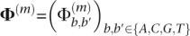 as the confusion matrix for position 1 ≤ m ≤ l, where l is the read length. It gives the probability that the true base is miscalled as another base given its position in the read. We later provide an EM procedure for estimating Φ(m) for 1 ≤ m ≤ l.
Let r denote a read, and suppose that the base at position m of r, which we denote rm, originated from position i of the genome S. In the absence of any sequencing error, read r will be identical to the substring H ≡ Si−m+1:i+l−m, where l is the length of the read, and Sa:b denotes the substring of S from position a to position b, inclusive. In other words, H is the “perfect” read that r would be if there were no sequencing errors. The entry  in the confusion matrix Φ(m) is defined as
the probability that the mth position of read r is called as b′ given that the true base is b. Note that Φ(m) is indexed by m, the called-base's position in the read. This is critical because the Illumina platform suffers from progressively worse accuracy toward the ends of its reads and, hence, it is essential to model this behavior statistically.
We use the following model for the distribution on observed reads:
Bases are distributed uniformly at random in the genome:
Every base is called independently, and the distribution on the called base depends on its position in the read and the true base:
Based on this model, we obtain the posterior distribution
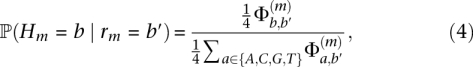 |
which gives the probability that, given we observe base b′ in a read, the true base is in fact b (which may or may not be the same as b′).
Now we use the assumption that overlaps of neighboring reads cover the same positions in the genome. For every position belonging to a particular overlap, we consider every read that contributes to the overlap. Each read provides its own base-call for that position, which is used to “sharpen” the posterior distribution described in Equation 4.
Let Ω = {(b1, p1), … } be the multiset of base-calls and their corresponding positions in reads that overlap with position m in read r. The posterior of Hm to be base b is then given by
 |
The maximum a posteriori (MAP) estimate of Hm is then
This MAP estimate of Hm is taken as the base at position m in read r. We perform this maximum a posteriori correction for all the reads in the data set. The procedure for handling a reverse complement read is analogous to the aforementioned steps.
Coverage checks
An abnormally large set of overlapping reads usually indicates nonuniform coverage or that the reads are sampled from a repetitive region, and suggests that our assumptions on overlapping reads most likely do not hold. From the overlaps found in the neighbor finding stage, we have an estimate of the expected coverage μ, as described in the Parameter selection. If the coverage at a position is greater than  (α standard deviations greater than the average coverage), we do not perform a correction. Our empirical study suggests that the precise value of α does not generally affect the accuracy of the algorithm; 4 ≤ α ≤ 6 is typically effective. This “filtering” allows ECHO to be robust against parts of the genome that have repetitive structure or have highly nonuniform coverage. We refer to this filtering as a “coverage check,” because it ensures that the estimated coverage for a read looks reasonable before correction is attempted.
Quality scores
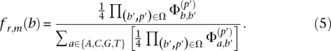
Providing an accurate measure of per-base quality has practical importance. For instance, MAQ (Li et al. 2008), a widely used read-mapping algorithm, utilizes base-specific quality scores to produce mapping quality scores and to call variants. A widely adopted definition of quality score is that used in phred (Ewing and Green 1998); it is a transformed error probability of a base, defined more precisely as follows: Let er,m denote the probability that rm, the mth base of read r, is erroneously called. Then, the phred quality score qr,m for rm is given by
Since ECHO provides an estimate of the posterior probability of each base, the error probability er,m of base  where rECHO denotes the ECHO-corrected read, can be estimated by
where fr,m (·) is defined as in Equation 5. The phred quality score for  is then obtained by using Equation 8 in Equation 7.
Generalization to diploid genomes
In this section, we show how our approach can be generalized to handle short reads from diploid genomes, in which case the main challenge lies in distinguishing heterozygotes from sequencing errors. We use the same neighbor-finding algorithm as in the haploid case, but modify the maximum a posteriori error-correction step as described below. Again, our exposition refers to the original reads; the case for reverse complements is analogous.
The unordered genotype at a given position of a diploid genome is either a homozygote or a heterozygote. We use Hom = {{A, A}, {C, C}, {G, G}, {T, T}} to denote the set of homozygous genotypes and Het = {{A, C}, {A, G}, {A, T}, {C, G}, {C, T}, {G, T}} to denote the set of heterozygous genotypes. The set of all possible genotypes is denoted by  .
.
Given a length-l haplotype sequence r = (r1,…,rl) ∈ {A, C, G, T}l, let 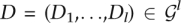 l denote the true unphased genotype sequence in the diploid genome from which r originated. Our goal is to assign a length-l unphased genotype sequence
  to each read r, such that
  is as close to D as possible. For each position m in r, we assume that the two alleles in D are equally likely to be the source of the mth nucleotide rm. Hence, sequencing errors at that position are characterized by the following generalized confusion matrix
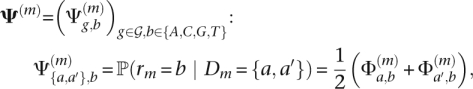 |
where {a, a′} is the true genotype, b is the base at position m in read r, and  is defined as in Equation 1.
We use h to denote the prior probability that a given site in the diploid genome is heterozygous. Then, for a particular genotype g ∈  , the prior is
 |
That is, given the zygosity, we assume the uniform distribution over all possible genotypes. Analogous to the haploid case, the posterior distribution is given by
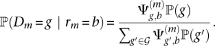 |
Let Ω = {(b1, p1), … } be the multiset of base-calls and their corresponding positions in reads that overlap with position m in read r. Then, the posterior of Dm being genotype g is
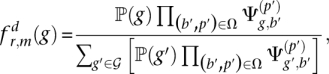 |
and the maximum a posteriori estimate of Dm is
In ECHO, this MAP estimate is taken to be the inferred genotype corresponding to position m of read r. As in the haploid case, if the estimated coverage at a particular position is much greater than the expected coverage, the maximum a posteriori estimate is not used and instead the algorithm outputs the genotype {rm, rm}, analogous to not correcting the base in the haploid case.
Let  be the sequence of genotypes estimated by ECHO for read r. The error probability for
  , the genotype at position m of
  , is
, is
and Equation 7 can be used to compute the quality score for  . Incidentally, note that the above algorithm for the diploid case with h = 0 reduces to the algorithm described earlier for the haploid case.
Estimating confusion matrices
If a reference genome is available, the confusion matrices Φ(m), for 1 ≤ m ≤ l, may be estimated by first aligning reads to the reference genome, treating mismatches as errors. However, this estimation can be biased, since mismatches may also originate from single nucleotide polymorphism or structural variations. Another method of estimating the confusion matrices is to use a control lane that sequences a known genome. This method avoids the potential biases caused by variations between the sampled genome and the reference genome, but this solution is costly and error characteristics can still differ between different lanes or runs.
Based on our probabilistic model, in which the true bases in the genome are unobserved latent variables, we adopt the EM algorithm to estimate confusion matrices. The advantage of the EM algorithm is that estimation can be performed without a reference genome. To start the estimation of Φ(m), for 1 ≤ m ≤ l, we first obtain the overlapping relationships between reads with the parameters k, ω*, and ε* as described in Neighbor finding and Parameter selection. Then, we fix the neighbor relationships and apply the EM algorithm, with the initial confusion matrix having 0.99 in the diagonal and 0.01/3 for all off-diagonal entries. The EM algorithm typically terminates after a few iterations.
Results
In this section, we evaluate the performance of our algorithm ECHO and compare it with previous error-correction methods. In particular, we consider the Spectral Alignment (SA) algorithm used in the preprocessing step of the de novo assembler EULER-USR (Chaisson et al. 2009). This error-correction algorithm is based on examining the k-mer spectrum of the input reads (Pevzner et al. 2001; Chaisson et al. 2004). Because SA is sensitive to the choice of k, for each experiment we ran SA over a range of k and selected the k that generated the optimal results (this was typically around k = 15).
SHREC (Schröder et al. 2009) is a recent error-correction algorithm based on a generalized suffix trie data structure; it essentially considers the substring spectrum of the input reads, i.e., a range of k-mers where k is over a given interval. It requires the user to specify the size of the genome, and we provided it with the true genome size for each data set we considered. Further, SHREC has a parameter called “strictness,” with the default value being 7. For coverage depths c <40, SHREC failed to run with the default parameter value, so we used the largest value less than seven that the program accepted. As discussed in the Methods, ECHO automatically chooses its parameters k, ω*, and ε*.
In addition to the improvement in data quality, we also examine the effects of error correction on de novo assembly.
Data and experiment setup
We tested the performance of our method on both real and simulated data over a range of coverage depths. Specifically, the following data sets were considered:
D1 (PhiX174)
We used standard resequencing data of the PhiX174 virus. The 76-bp reads were obtained from the Illumina GA-II platform, with the viral sample in a single lane of the flow cell. The length of the PhiX174 genome is 5386 bp, and the short-read data had a coverage depth of around 210,000. In our experiments, various coverage depths were obtained by sampling without replacement from the actual data set. We used Illumina's standard base-calling software, Bustard, to produce base-calls. To create labeled test data, we aligned the reads against the reference genome and regarded every mismatch as a sequencing error.
D2 (D. mel.)
Another real data set we used is that of D. melanogaster inbred line RAL-399, sequenced and assembled by the Drosophila Population Genomics Project (DPGP, http://www.dpgp.org/). The short-reads were downloaded from the NCBI Sequence Read Archive (http://www.ncbi.nlm.nih.gov/Traces/sra/sra.cgi). The data consisted of 36-bp reads sequenced on the Illumina GA I platform and base called by Bustard. The overall coverage depth of the data set was roughly 13. To create a labeled test set, we aligned the reads against the genome assembly (release 1.0) produced by DPGP. Then, we selected the reads that mapped to chromosome 2L and regarded mismatches as sequencing errors.
D3 (Simulated D. mel.)
In the test described above in D2, errors in the assembled genome (i.e., differences between the assembled genome and the true genome) may confound the assessment of the accuracy of error-correction algorithms. To avoid this potential problem, we generated 76-bp simulated reads from a 100-kbp or a 5-Mbp region of chromosome 2L of the RAL-399 inbred line mentioned above. To simulate each 76-bp read, we chose a starting position uniformly at random from the chosen region or its reverse complement, and introduced errors by selecting a random “error template” as follows: First, we selected a read randomly from the PhiX174 data set D1 and aligned it to the PhiX174 reference genome to determine the positions of errors. Then, we took that error template and added errors to the simulated Drosophila read at the corresponding locations. The miscalled base was determined according to the position-specific empirical confusion matrices estimated from the PhiX174 data, because the “error template” from the sampled PhiX174 read only provides the positions of errors. This approach allowed us to simulate more realistic error patterns; e.g., the correlation of errors in a read and the clustering of errors on a subset of the reads. Our simulation method permitted miscall errors, but no indels.
D4 (Simulated human data with repeats and duplicated regions)
To evaluate the performance of ECHO on sequences with repeats and duplicated regions, we generated 76-bp reads from a 250-kbp region of human chromosome 16 known to have a duplicated gene (Martin et al. 2004). More specifically, the region spans chromosomal coordinates 20,240,000–20,490,000 of the GRCh37 reference assembly of chromosome 16, downloaded from the NCBI Genome database. We followed the same procedure as in D3 setup to introduce errors into reads randomly selected from the 250-kbp region.
D5 (Simulated diploid data)
To generate a known diploid genome, we took the 100-kbp region mentioned in D3 and mutated each base with probability 0.001, with the new base drawn uniformly at random from the alternative bases. To simulate each 76-bp read, we followed the same procedure as in D3 to add errors to a randomly sampled read from the diploid strands and their reverse complements. For this diploid data set, the sequence coverage depth is given by  where N denotes the number of reads, l = 76, and L = 100,000.
D6 (Saccharomyces cerevisiae)
This real data set consisted of 7.1 million reads from the whole-genome sequencing of a laboratory-evolved yeast strain derived from DBY11331 (Gresham et al. 2008), Accession Number SRR031259 in the NCBI Sequence Read Archive. Because the yeast strain differed slightly from the S. cerevisiae reference genome, we created a new assembly using MAQ (Li et al. 2008) and the standard reference sequence. We used this newly assembled genome to evaluate error-correction performance in our experiments. The data set contained single-end 36-bp reads from the Illumina GA II platform, covering all 16 chromosomes and the mitochondrial DNA of S. cerevisiae. The overall coverage depth of the data set was roughly 21.
Error-correction accuracy for haploid genomes
We compared the error-correction accuracy of SA, SHREC, and ECHO on the data sets described in the previous section. Because the output of SHREC is partitioned into “corrected” and “discarded” reads, we measured the performance of SHREC by considering only the corrected reads.
Following, we use the term by-base error rate to refer to the ratio of the total number of incorrect bases in the reads to the total combined length of the reads. We also consider the by-read error rate, which corresponds to the ratio of the number of reads with at least one miscalled base to the total number of reads. Table 1 shows the by-base and by-read error rates for haploid data sets D1–D4 before and after running the three error-correction algorithms. On all data sets, ECHO was more effective than SA and SHREC at reducing the error rates. In general, SA did not seem effective at reducing the by-base error rate. SHREC was more effective than SA, whereas our algorithm improved on SHREC by several folds on both real and simulated data. Table 2 shows the numbers of corrected errors and introduced errors, as well as the gain, for the same data sets after error correction. The gain is defined as the number of corrected errors minus the number of introduced errors, divided by the number of actual errors, in the same manner as in Yang et al. (2010). As the table shows, the gain for ECHO was substantially higher than that for SA or SHREC.
Table 1.
Error rates for haploid data before and after running error correction

Table 2.
Numbers of corrected errors and introduced errors after running error correction

Observe that all three algorithms generally improved the by-read error rates noticeably, with ECHO being more effective than both SA and SHREC. It is interesting that while SA only moderately improved the by-base error rate, it was effective at improving the by-read error rate.
To compare the performance of the three error-correction algorithms in more detail, we examined the position-specific by-base error rates; i.e., the by-base error rate at position i is the ratio of the number of reads with an incorrect base at position i to the total number of reads. For PhiX174 data D1 with experiment setup with sequence coverage depth 30, see Figure 3A, which illustrates the position-specific by-base error rates before and after applying the error-correction algorithms. It is well-known that the error rate of the Illumina platform generally increases toward the end of the read, reaching as high as 5% in the example shown. Although SA and SHREC were able to reduce this effect to a certain degree, they both became less effective for later positions. In contrast, ECHO remained quite effective throughout the entire read length. In particular, the error rate at the end of the read was reduced from about 5% to <1%.
Figure 3.

Position-specific by-base error rates for 76-bp PhiX174 data D1. (A) Error rates before and after applying the three error-correction algorithms for sequence coverage depth 30. Spectral alignment (or SA) (see Chaisson et al. 2009) and SHREC (Schröder et al. 2009) are able to improve the error rate in intermediate positions, but they both become less effective for later positions. In contrast, ECHO remains effective throughout the entire read length, reducing the error rate at the end of the read from about 5% to under 1%. (B) Error rates before and after running ECHO with varying coverage depths. ECHO's ability to correct sequencing errors improves as the sequence coverage depth increases. A coverage depth of 15 seems sufficient to control the error rate throughout the entire read length.
We considered the effect of coverage depth on the performance of our algorithm. Figure 3B shows the position-specific by-base error rates before and after applying ECHO on PhiX174 data with varying sequence coverage depths. At a coverage depth of 15, the error rate could be controlled throughout the entire read length, resulting in only a slight increase in the error rate toward the end of the read.
Although ECHO improved on the other error-correction methods on the simulated human data set D4 (see Tables 1, 2), the improvement was not as pronounced as for the Drosophila and PhiX174 data sets. This demonstrates that ECHO is most effective on genomes with limited repetitive structure. Although the read overlap approach might be less susceptible to repeat regions than a k-mer spectrum method, it does not adequately overcome this obstacle. Further work is required to handle repeat regions, which are common in more complex genomes, such as mammalian genomes.
Whole-genome error correction
To evaluate the performance of ECHO on whole-genome data, we ran an experiment on the yeast data D6. Results from the experiment are shown in Tables 3 and 4. The performance of all evaluated error-correction algorithms was noticeably worse for this data set than for the others. Closer examination of the data revealed that the mitochondrial DNA (mtDNA) had much higher coverage than the other chromosomes, 210× compared with 19.5×. Because ECHO compares a read's estimated coverage to the estimated coverage over the entire genome, nearly every read from the mtDNA was not corrected. This contrasts with SHREC, which does not account for such drastic differences in coverage across the genome. This suggests that although ECHO assumes uniform coverage of the genome when determining its parameters, when it encounters data with highly nonuniform coverage, it avoids confusion caused by the nonuniform coverage by requiring the reads to pass the coverage checks described earlier. It should be noted that repetitive structure would also cause a read not to pass the coverage check, which would cause ECHO to be more conservative around repeat regions.
Table 3.
Error rates for the whole-genome yeast data D6

Table 4.
Numbers of corrected errors and introduced errors after running error correction on the whole-genome yeast data D6

To better quantify the performance of the error-correction algorithms, we divided the data set into two groups: reads that passed the coverage checks and those that did not. Restricted to those reads that passed the coverage checks (i.e., the reads on which error correction was actually attempted), ECHO was able to reduce the by-base error rate from 1.28% to 0.83% (which corresponds to about 35% improvement), while reducing the by-read error rate from 17.3% to 8.4%. Hence, ECHO's performance on this restricted read set was almost as good as that for the other real data sets (e.g., D1 and D2). By comparison, for the reads on which SHREC attempted error correction, it was able to reduce the by-base error rate from 0.89% to 0.79% (which corresponds to about 11% improvement), while reducing the by-read error rate from 14.8% to 10.6%. SA did not make any error correction on this data set.
Figure 4 shows the gain for ECHO and the coverage along chromosome 1. As mentioned before, the gain corresponds to the number of corrected errors minus the number of introduced errors, divided by the number of actual errors. The plots illustrate that when the coverage increases significantly, the gain tends to drop. This is because the reads from these positions generally do not pass the coverage checks ECHO imposes.
Figure 4.

The gain of ECHO and the position-specific coverage for chromosome 1 of the yeast data D6. Each plot uses bins of 1000 bp. The top plot shows the gain of ECHO, defined as the number of corrected errors minus the number of introduced errors, divided by the number of actual errors. The bottom plot shows the position-specific coverage.
Table 4 illustrates that SHREC corrected about 1.5 times more bases than did ECHO, but the number of errors introduced by SHREC was 41 times greater than that introduced by ECHO. As a result, the gain for ECHO was higher than that for SHREC. Because of the coverage checks it performs, ECHO was more conservative in correcting reads coming from highly covered regions of the genome. We expect this to be an advantageous feature of ECHO, as a high estimated coverage is often indicative of repeat structure.
Robustness with respect to the choice of the keyword length k
In the Methods, under Parameter selection, we provided a rough guideline for choosing the keyword length k in the neighbor finding algorithm. Here, we show empirically that the performance of ECHO with the suggested setting k = [l/6], with l being the read length, is comparable to the performance of the algorithm with the optimal k that maximizes the error-correction performance.
For this study, we subsampled reads from data D3 to create a data set consisting of 25,000 reads of length 76 bp. This corresponds to a sequence coverage depth of 19. The average by-base error rate in the simulated reads was around 1%. For each given k, we used the method described in Parameter selection to determine ω* and ε*. These parameters, k, ω*, and ε*, were then used to perform error correction on the reads. For the simulated data we considered, the value of k that led to the largest improvement in the error rate was k = 7, in which case, ECHO reduced the error rate from 1% to 0.107%. By comparison, the associated error rate for k = [l/6] = 12 was 0.109%, which is comparable to the optimal case.
Error-correction accuracy for diploid genomes
As described in the Methods, ECHO can handle diploid data as well as haploid data. Recall that ECHO explicitly models heterozygosity in diploid genomes and has a parameter, denoted h, corresponding to the probability that a given site is heterozygous. Setting h = 0 reduces the model to the haploid case. Neither SA nor SHREC explicitly models diploidy, so they may be compared with the case of h = 0 in our model.
We tested the methods on simulated diploid data D5. In simulating the diploid genome, the probability of heterozygosity was set to 10−3 for each site. Table 5 shows a summary of error-correction results on diploid data D5. As in the haploid case, SA was not effective in reducing the by-base error rate, though it was able to reduce the by-read error rate reasonably well. SHREC significantly improved on SA in terms of the by-base error rate, whereas their by-read error rates were comparable. ECHO with h = 0 improved on both SA and SHREC by several folds for coverages 30 and higher. For these coverage depths, ECHO reduced the by-read error rate from around 27% to about 2%. The improvement in the by-base error rate was equally significant in proportion. For h > 0, ECHO displayed accuracy greater than that for h = 0, demonstrating the utility of explicitly modeling the diploidy of the genome.
Table 5.
Error rates for diploid data D5 before and after error correction

Table 6 shows the detection accuracy of heterozygous sites in the diploid data. The precision and recall are shown for varying levels of coverage and for both h = 10−3 and h = 10−4. Precision and recall are commonly used performance measurements in information retrieval tasks. In this context, precision is the number of correctly called heterozygous sites divided by the number of all called heterozygous sites (including incorrectly called heterozygous sites), and recall is the number of called heterozygous sites divided by all true heterozygous sites.
Table 6.
Heterozygous site detection efficiency for simulated diploid data D5

Every genotype called by ECHO is given a quality score. As illustrated in Table 6, we can trade off recall for higher precision by filtering based on quality. These results demonstrate that, with high enough coverage, ECHO provides a reliable reference-free method of detecting bases that originated from heterozygous sites and inferring the corresponding genotypes.
Effects on de novo assembly
Intuitively, improved data quality should facilitate assembly. To assess the effects of various error-correction methods on de novo assembly, we used Velvet (Zerbino and Birney 2008) to carry out the assembly. Like many other de novo assembly algorithms, Velvet is based on k-mers and the associated de Bruijn graph representation. In each experiment, we used k = 39 and automatic coverage cutoff, and provided Velvet with the true expected coverage.
The data sets we considered were real PhiX174 data D1 and experiment setup and simulated data D3 from a 5-Mbp region of D. melanogaster; the former experiment was repeated 20 times, while the latter was repeated twice.
For the PhiX174 data set, Velvet was run on the following four sets of short-reads:
Uncorrected reads, corresponding to the original simulated reads.
Error-corrected reads processed by SA, SHREC, or ECHO.
For the simulated D. melanogaster data sets, Velvet was also run on the following set of short-reads, in addition to the above four sets:
Perfect reads, corresponding to the error-free reads from which the uncorrected reads were simulated.
The results for PhiX174 are shown in Table 7, where “Max” denotes the maximum contig length, and “N50,” defined in the caption, is a statistic commonly used to assess the quality of de novo assembly. Larger values of Max and N50 indicate better assembly quality. For nearly all sequence-coverage depths, note that using ECHO-corrected reads led to the largest Max and N50 values.
Table 7.
De novo assembly results for uncorrected and corrected PhiX174 data D1

The assembly results for simulated 5-Mbp D. melanogaster data are summarized in Table 8. There was a clear advantage to performing error correction prior to assembly, and error correction produced an appreciable improvement over uncorrected reads. In addition to Max and N50, we assessed the assembly quality using the following two new measures:
Table 8.
De novo assembly results for simulated data D3 from a 5-Mbp region of D. melanogaster

SeqCov1000 is the percentage of the genome covered by the contigs of length ≥1000 bp.
Error1000 is the percentage of the total number of assembly errors (measured by edit distance from the true genome, with a penalty of 1 for mismatch, insertion, or deletion) in those contigs with length ≥1000 bp, with respect to the total length of those contigs.
For coverage depths ≥20, SeqCov1000 values for all three error-correction methods were comparable to that for perfect reads.
As Tables 7 and 8 illustrate, the key advantage of ECHO is its consistency; i.e., the performance of ECHO is consistently good for all coverage depths and all data sets, while the other error-correction methods seem more erratic (e.g., see the performance of SHREC in Table 7, and the performance of SA in Table 8 for coverages ≥20).
Running times
We ran the three error-correction algorithms on simulated data from the D. melanogaster reference sequence to compare their running times. We fixed the sequence coverage depth at 20 and varied the genome length to adjust for different quantities of reads. Errors were added to the reads in the same way as in D3. All experiments were done on a Mac Pro with two quad-core 3.0 GHz Intel Xeon processors and 14 GB of RAM. SA and ECHO each used only a single core, whereas SHREC was allowed to use all eight cores.
Shown in Table 9 is a summary of running times. Since our algorithm needs to determine the parameters ω* and ε*, its running time is divided into two parts: parameter selection time, shown in parentheses, and the running time for neighbor finding and error correction. Although our algorithm is slower, note that its running time is within the range of practical use. On the whole-genome yeast data D6 discussed earlier, SA took 6 min and SHREC took 37 min, while ECHO took 260 min. (Recall that SA did not make any error correction on this data set.)
Table 9.
Comparison of running times, in minutes, for simulated data with 76-bp reads

If the entire adjacency list for the overlaps between reads can be stored in memory, the running time of ECHO scales linearly in the number of reads, provided that k is chosen large enough such that the number of reads that contain a given k-mer scales linearly in the coverage depth. In our experiments, ECHO was given k = ⌊l/6⌋ = 12.
On the other hand, if the available amount of memory is not sufficient, our implementation first partitions the read set into smaller subsets. Then, successively, for the partitioned reads the adjacency lists for the read overlaps are constructed and then merged in a tree-like fashion. Error correction is then performed on the reads while reading in only a small portion of the adjacency list at a time, reducing memory usage significantly. Using this approach and assuming the number of repeat regions in the genome is not too high, the running time of ECHO scales approximately as O(N log N), where N is the number of reads.
Discussion
In this study, we introduced a new reference-free error-correction algorithm, ECHO, for correcting sequencing errors in short reads. It has several important novel features. One advantage of ECHO over previous methods is that it does not rely on the user to specify many of the key parameters; this is an important feature since the optimal parameter values for given input data are typically unknown to the user a priori. Without the need of a reference genome, ECHO efficiently clusters those reads that may have originated from the same region of the genome, and automatically sets the parameters in the assumed model. Moreover, being based on a probabilistic framework, ECHO can assign a quality score to each corrected base; we are not aware of any other reference-free error-correction algorithm that also does this.
Another novel feature of ECHO is that it explicitly models heterozygosity in diploid genomes. This allows for the detection of bases that originated from heterozygous sites in the sequenced diploid genome and to infer the corresponding genotypes without using a reference genome. We leave as future research utilizing this information in downstream computational problems, including polymorphism detection and assembly.
The improvement in data quality delivered by our algorithm is most pronounced toward the end of the read, where previous methods become considerably less effective. In the Illumina platform, the error rate generally increases toward the end of the read. However, provided that the sequence coverage depth is sufficiently high, ECHO is able to control the error rate to stay at <1% throughout the entire read length (see Fig. 3A,B). This suggests that one possible way to obtain longer reads for a given error tolerance is to allow the sequencing machine to run beyond that tolerance level and then apply an error-correction algorithm afterward to reduce the error rate. This kind of strategy should help to relax the limitation on the read length imposed by the imperfectness of the chemical process.
Similar to previous error-correction algorithms, ECHO is typically most effective on genomes without complex repeat structure, such as bacterial and other nonmammalian genomes. Although ECHO has several mechanisms to avoid correcting repetitive regions, such as ignoring reads with an abnormally large number of overlaps and setting the minimum overlap high enough such that the coverage distribution is Poisson distributed, repetitive regions still lead to a greater number of false overlaps, thus confounding the error-correction process.
As an application to de novo assembly, we demonstrated that error correction can provide significant improvements in the quality of the resulting contigs. In particular, we showed that for low-to-moderate coverage depths, performing error correction prior to assembly may significantly improve the quality of de novo assembly. It will be interesting to explore whether reference-free error correction may facilitate de novo transcriptome assembly (Birol et al. 2009).
The method described in this study may be improved in a few ways. (1) In parameter selection, we assumed that the number of neighbors that overlap with any particular position in a given read is Poisson distributed. In practice, this may not be a very good assumption, and using a different distribution for fitting might lead to better choices of ω* and ε*. (2) Instead of using a subset of reads randomly chosen from the input set of reads, it may improve parameter selection if the subset is chosen more judiciously; e.g., by filtering out the reads with repeats. (3) The short-reads generated by most NGS platforms come with base-specific quality scores, but ECHO currently does not utilize that information. It is possible to incorporate per-base quality scores into ECHO, thereby further improving its accuracy. (4) Our current implementation of the neighbor-finding algorithm assumes that indel errors are rare, as is the case for the Illumina platform. For the sequencing platforms with high indel error rates (e.g., Roche's pyrosequencing technology), the alignment step in the neighbor-finding algorithm needs to be generalized to include indels. However, the overall idea underlying ECHO is still applicable.
Acknowledgments
We thank Satish Rao, Aileen Chen, Nanheng Wu, and Jerry Hong for useful discussions. This research is supported in part by an NSF CAREER Grant DBI-0846015, an Alfred P. Sloan Research Fellowship, and a Packard Fellowship for Science and Engineering to Y.S.S.; and by a National Defense Science & Engineering Graduate (NDSEG) Fellowship to A.H.C.
Footnotes
[Supplemental material is available for this article. ECHO is publicly available at http://uc-echo.sourceforge.net under the Berkeley Software Distribution License.]
Article published online before print. Article, supplemental material, and publication date are at http://www.genome.org/cgi/doi/10.1101/gr.111351.110.
References
- Batzoglou S, Jaffe DB, Stanley K, Butler J, Gnerre S, Mauceli E, Berger B, Mesirov JP, Lander ES 2002. Arachne: a whole-genome shotgun assembler. Genome Res 12: 177–189 [DOI] [PMC free article] [PubMed] [Google Scholar]
- Birol I, Jackman S, Nielsen C, Qian J, Varhol R, Stazyk G, Morin R, Zhao Y, Hirst M, Schein J, et al. 2009. De novo transcriptome assembly with ABySS. Bioinformatics 25: 2872–2877 [DOI] [PubMed] [Google Scholar]
- Brockman W, Alvarez P, Young S, Garber M, Giannoukos G, Lee WL, Russ C, Lander ES, Nusbaum C, Jaffe DB, et al. 2008. Quality scores and SNP detection in sequencing-by-synthesis systems. Genome Res 18: 763–770 [DOI] [PMC free article] [PubMed] [Google Scholar]
- Butler J, MacCallum I, Kleber M, Shlyakhter IA, Belmonte MK, Lander ES, Nusbaum C, Jaffe DB 2008. ALLPATHS: De novo assembly of whole-genome shotgun microreads. Genome Res 18: 810–820 [DOI] [PMC free article] [PubMed] [Google Scholar]
- Chaisson M, Pevzner P, Tang H 2004. Fragment assembly with short reads. Bioinformatics 20: 2067–2074 [DOI] [PubMed] [Google Scholar]
- Chaisson MJP, Brinza D, Pevzner PA 2009. De novo fragment assembly with short mate-paired reads: Does the read length matter? Genome Res 19: 336–346 [DOI] [PMC free article] [PubMed] [Google Scholar]
- Chin F, Leung H, Li W-L, Yiu S-M 2009. Finding optimal threshold for correction error reads in DNA assembling. BMC Bioinformatics (Suppl 1) 10: S15 doi: 10.1186/1471-2105-10S1-15 [DOI] [PMC free article] [PubMed] [Google Scholar]
- Erlich Y, Mitra P, Delabastide M, McCombie W, Hannon G 2008. Alta-Cyclic: a self-optimizing base caller for next-generation sequencing. Nat Methods 5: 679–682 [DOI] [PMC free article] [PubMed] [Google Scholar]
- Ewing B, Green P 1998. Base-calling of automated sequencer traces using Phred. II. Error probabilities. Genome Res 8: 186–194 [PubMed] [Google Scholar]
- Gajer P, Schatz M, Salzberg SL 2004. Automated correction of genome sequence errors. Nucleic Acids Res 32: 562–569 [DOI] [PMC free article] [PubMed] [Google Scholar]
- Gresham D, Desai MM, Tucker CM, Jenq HT, Pai DA, Ward A, DeSevo CG, Botstein D, Dunham MJ 2008. The repertoire and dynamics of evolutionary adaptations to controlled nutrient-limited environments in yeast. PLoS Genet 4: e1000303 doi: 10.1371/journal.pgen.1000303 [DOI] [PMC free article] [PubMed] [Google Scholar]
- Hellmann I, Mang Y, Gu Z, Li P, Vega FMDL, Clark AG, Nielsen R 2008. Population genetic analysis of shotgun assemblies of genomic sequences from multiple individuals. Genome Res 18: 1020–1029 [DOI] [PMC free article] [PubMed] [Google Scholar]
- Jiang R, Tavare S, Marjoram P 2009. Population genetic inference from resequencing data. Genetics 181: 187–197 [DOI] [PMC free article] [PubMed] [Google Scholar]
- Jokinen P, Ukkonen E 1991. Two algorithms for approximate string matching in static texts. In Proceedings of Mathematical Foundations of Computer Science. Lect Notes Comput Sci 520: 240–248 [Google Scholar]
- Kao W-C, Song Y 2010. naiveBayesCall: An efficient model-based base-calling algorithm for high-throughput sequencing. In Proceedings of the 14th Annual International Conference on Research in Computational Molecular Biology (RECOMB). Lect Notes Comput Sci 6044: 233–247 [DOI] [PubMed] [Google Scholar]
- Kao W-C, Stevens K, Song YS 2009. BayesCall: A model-based basecalling algorithm for high-throughput short-read sequencing. Genome Res 19: 1884–1895 [DOI] [PMC free article] [PubMed] [Google Scholar]
- Kircher M, Stenzel U, Kelso J 2009. Improved base calling for the Illumina Genome Analyzer using machine learning strategies. Genome Biol 10: R83 doi: 10.1186/gb-2009-10-8-r83 [DOI] [PMC free article] [PubMed] [Google Scholar]
- Langmead B, Trapnell C, Pop M, Salzberg S 2009. Ultrafast and memory-efficient alignment of short DNA sequences to the human genome. Genome Biol 10: R25 doi: 10.1186/gb-2009-1-3-r25 [DOI] [PMC free article] [PubMed] [Google Scholar]
- Li H, Durbin R 2010. Fast and accurate long-read alignment with Burrows-Wheeler transform. Bioinformatics 26: 589–595 [DOI] [PMC free article] [PubMed] [Google Scholar]
- Li H, Ruan J, Durbin R 2008. Mapping short DNA sequencing reads and calling variants using mapping quality scores. Genome Res 18: 1851–1858 [DOI] [PMC free article] [PubMed] [Google Scholar]
- Martin J, Han C, Gordon LA, Terry A, Prabhakar S, She X, Xie G, Hellsten U, Chan YM, Altherr M, et al. 2004. The sequence and anslysis of duplication-rich chromosome 16. Nature 432: 988–994 [DOI] [PubMed] [Google Scholar]
- Medvedev P, Brudno M 2008. Ab initio whole genome shotgun assembly with mated short reads. In Proceedings of the 12th Annual International Conference on Research in Computational Molecular Biology (RECOMB). Lect Notes Comput Sci 4751: 50–64 [Google Scholar]
- Metzker M 2010. Sequencing technologies–the next generation. Nat Rev Genet 11: 31–46 [DOI] [PubMed] [Google Scholar]
- Peng Y, Leung H, Yiu S, Chin F 2010. IDBA - A practical iterative de Bruijn graph de novo assembler. In Proceedings of the 14th Annual International Conference on Research in Computational Molecular Biology (RECOMB). Lect Notes Comput Sci 6044: 426–440 [Google Scholar]
- Pevzner PA, Tang H, Waterman MS 2001. An Eulerian path approach to DNA fragment assembly. Proc Natl Acad Sci 98: 9748–9753 [DOI] [PMC free article] [PubMed] [Google Scholar]
- Qu W, Hashimoto S-i, Morishita S 2009. Efficient frequency-based de novo short-read clustering for error trimming in next-generation sequencing. Genome Res 19: 1309–1315 [DOI] [PMC free article] [PubMed] [Google Scholar]
- Rasmussen KR, Stoye J, Myers EW 2005. Efficient q-gram filters for finding all epsilon-matches over a given length. In Proceedings of the 9th Annual International Conference on Research in Computational Molecular Biology (RECOMB). Lect Notes Comput Sci 3678: 189–203 [DOI] [PubMed] [Google Scholar]
- Rougemont J, Amzallag A, Iseli C, Farinelli L, Xenarios I, Naef F 2008. Probabilistic base calling of Solexa sequencing data. BMC Bioinformatics 9: 431 doi: 10.1186/1471-2105-9-431 [DOI] [PMC free article] [PubMed] [Google Scholar]
- Salmela L 2010. Correction of sequencing errors in a mixed set of reads. Bioinformatics 26: 1284–1290 [DOI] [PubMed] [Google Scholar]
- Sanger F, Nicklen S, Coulson A 1977. DNA sequencing with chain-terminating inhibitors. Proc Natl Acad Sci 74: 5463–5467 [DOI] [PMC free article] [PubMed] [Google Scholar]
- Schröder J, Schröder H, Puglisi SJ, Sinha R, Schmidt B 2009. SHREC: a short-read error correction method. Bioinformatics 25: 2157–2163 [DOI] [PubMed] [Google Scholar]
- Shi H, Schmidt B, Liu W, Muller-Wittig W 2009. Accelerating error correction in high-throughput short-read DNA sequencing data with CUDA. In Proceedings of the IEEE International Parallel & Distributed Processing Symposium, pp. 1–8 Nanyang Technical University, Singapore [Google Scholar]
- Simpson JT, Wong K, Jackman SD, Schein JE, Jones SJ, Birol I 2009. ABySS: a parallel assembler for short read sequence data. Genome Res 19: 1117–1123 [DOI] [PMC free article] [PubMed] [Google Scholar]
- Sundquist A, Ronaghi M, Tang H, Pevzner P, Batzoglou S 2007. Whole-genome sequencing and assembly with high-throughput, short-read technologies. PLoS ONE 2: e484 doi: 10.1371/journal.pone.0000484 [DOI] [PMC free article] [PubMed] [Google Scholar]
- Whiteford N, Skelly T, Curtis C, Ritchie M, Lohr A, Zaranek A, Abnizova I, Brown C 2009. Swift: Primary data analysis for the Illumina Solexa sequencing platform. Bioinformatics 25: 2194–2199 [DOI] [PMC free article] [PubMed] [Google Scholar]
- Wijaya E, Frith MC, Suzuki Y, Horton P 2009. Recount: expectation maximization based error correction tool for next generation sequencing data. Genome Inform 23: 189–201 [PubMed] [Google Scholar]
- Yang X, Dorman KS, Aluru S 2010. Reptile: representative tiling for short read error correction. Bioinformatics 26: 2526–2533 [DOI] [PubMed] [Google Scholar]
- Zerbino DR, Birney E 2008. Velvet: Algorithms for de novo short read assembly using de Bruijn graphs. Genome Res 18: 821–829 [DOI] [PMC free article] [PubMed] [Google Scholar]