Understanding the Early Origins of the Education–Health Gradient: A Framework That Can Also Be Applied to Analyze Gene–Environment Interactions

Abstract

In this article, we develop a framework for analyzing the causal effects of interventions in the presence of latent factors that could affect outcomes, even in the absence of interventions. This framework will be useful in situations in which genes are included among the latent factors. We estimate the model and study the early origins of observed later-life disparities by education. We determine the role played by cognitive, noncognitive, and early health endowments. We identify the causal effect of education on health and health-related behaviors. We show that family background characteristics and cognitive, noncognitive, and health endowments developed by age 10 are important determinants of health disparities at age 30. We also show that not properly accounting for personality traits results in overestimation of the importance of cognitive ability in determining later health. Selection on preexisting traits explains more than half of the observed differences in poor health and obesity. Education has an important causal effect in explaining differences in smoking rates. There are significant gender differences. We go beyond the current literature, which typically estimates mean effects, to compute distributions of treatment effects. We show that the effect of education on health varies among individuals who are similar in their observed characteristics, and how a mean effect can hide gains and losses for different individuals. This analysis highlights the crucial role played by promotion of good health at an early age and the importance of prevention in the reduction of health disparities. We speculate about how the model can be applied to genetic studies.

Background

Researchers are paying increasing attention to the social determinants of health and placing growing emphasis on the value of early childhood interventions (Commission on Social Determinants of Health, 2008; Currie, 2009b; Marmot, 2010). Recent studies suggest that early endowments, including genes, play an important role in understanding the etiology and the evolution of health disparities (Bamshad, 2005; Fine, Ibrahim, & Thomas, 2005). Genes and other factors set early in life may determine the choice of education, lifestyles, and environments that are beneficial or detrimental to health. Observed health differences in individuals living in different environments may reflect, in part, heterogeneity in these early endowments. They may also play a role in determining differential responses to interventions and choices across individuals otherwise similar in their observed characteristics.¹

A growing literature establishes strong relationships between early childhood conditions and adult outcomes (Knudsen, Heckman, Cameron, & Shonkoff, 2006). Gaps in both cognitive and noncognitive abilities across different families emerge at an early age (Cunha, Heckman, Lochner, & Masterov, 2006), as do gaps in health (Case, Lubotsky, & Paxson, 2002). Various studies suggest it is possible to partially compensate children damaged by adverse environments (Heckman, Moon, Pinto, Savelyev, & Yavitz, 2010). Very little research has focused on the role of these early factors on later health—there is still much to know. Our research aims to start to fill this gap.

We present a general framework that allows for both cognitive, noncognitive, and health factors and the choices of lifestyles, education, and environments to affect health outcomes. The concept of developmental health, comprising physical, genetic, cognitive, and psychosocial dimensions of child development, has been influential in life-course epidemiology (Davey Smith, 2003; Kuh & Ben-Shlomo, 1997), but it has not yet been fully accepted into the mainstream economics or medical literatures (McCormick, 2008).

In previous work (Conti, Heckman, & Urzua, 2010a, 2010b), we study the early origins of the education–health gradient. Health gaps between education groups are rising (Meara, Richards, & Cutler, 2008). Many authors have noted that better health early in life is associated with higher educational attainment (Currie, 2009a; Grossman, 1975; Perri, 1984; Wolfe, 1985), and that more educated individuals, in turn, have better health later in life and better labor market prospects (Cutler & Lleras-Muney, 2010; Grossman & Kaestner, 1997). A positive correlation between health and schooling is one of the most well-established findings in the social sciences (Kolata, 2007). However, whether and to what extent this correlation reflects causality is still subject to debate (see Grossman, 2000, 2006, for comprehensive reviews of the literature). Three explanations are offered in the literature: (a) causality runs from education to health (Grossman, 1972, 2008); (b) causality runs from health to education (Currie, 2009a); and (c) both health and education are determined by a third factor, such as time or risk preferences (Fuchs, 1982). Understanding the relative importance of each of these mechanisms in generating observed differences in Health × Education interactions is relevant to designing policies to promote health.

Much of the literature in epidemiology and public health decomposes health disparities by education without taking into account the fact that people make different educational choices on the basis of factors that are also determinants of health behaviors. The literature in economics addresses this problem largely using instrumental variables (Currie & Moretti, 2003; Lleras-Muney, 2005). This article examines the origins of health disparities by education in the context of a general framework of latent variables to analyze the effect of interventions and to disentangle causality from selection effects.

The paper is organized as follows: We first present a model of choice of schooling, lifestyles, and environments, which can, in principle, incorporate the role of genetics. We then motivate our empirical analysis, which summarizes the research of Conti, Heckman and Urzua (2010a, 2010b). Data and empirical results are then discussed. We next show how to estimate the causal effects of education on health and report estimates. We follow this discussion with possible application to genetics.

A Causal Model with Latent Factors Determining Outcomes and Choices of Education, Lifestyles, and Environments

This section presents a framework for causal analysis, developed in Carneiro, Hansen, and Heckman (2003); Aakvik, Heckman, and Vytlacil (2005); and Abbring and Heckman (2007). An agent at age t is characterized by a vector of capabilities:

$${\theta }_t=({\theta }_{Ct},{\theta }_{Nt},{\theta }_{Ht},{\theta }_G),$$

where θ_Ct is a vector of cognitive capabilities, θ_Nt is a vector of noncognitive capabilities, θ_Ht is a vector of health stocks, and θ_G is a genetic determinant. The latent factors in θ_t can evolve over time and may be governed by investment decisions (see Cunha & Heckman, 2008, 2009; Cunha, Heckman, & Schennach, 2010). We discuss how to introduce the genetic factor into analyses later in this article. For now, θ_G is just another latent factor.

A Latent Variable Model of Choice and Outcomes

Let $S_i^{*}$ denote the net utility an individual derives from selecting a certain environment and D_i denote a binary variable indicating his or her actual decision (so D_i = 1 if the individual selects that environment and D_i = 0 otherwise). Thus, we assume:

$$D_i=1\text{if}{S}_i^{*}\ge 0,D_i=0\text{otherwise}.$$ (1)

The net utility $S_i^{*}$ is determined by an individual's observed and unobserved characteristics:

$$S_i^{*}={\mu }_S(Z_i)+V_i,$$

where Z_i is a vector of observed characteristics determining an individual’s net utility level and V_i is an unobserved random variable that also affects utility. Z_i and V_i are assumed to be statistically independent conditional on X.

Once the individual has selected her environment, all future outcomes are potentially causally related to this decision. Our model allows individuals to choose their environments, taking into account the potential outcomes in the two possible states (exposed and unexposed).² This feature of our model is extremely important. To the extent that individuals select their environments anticipating future outcomes, we need to control for the potential consequences of selection when comparing outcomes across levels of exposures (i.e., comparisons of the outcomes of individuals exposed and unexposed are not informative on causal questions because the two samples are not random samples of the potential outcomes in the population for each state). We deal with the selection problem by using a model of potential outcomes due to Neyman (1923) as extended in economics to model the choices of the environments made by the agents (e.g., Heckman & Sedlacek, 1985; Roy, 1951) In this model, observed and unobserved variables (unobserved from the point of view of the researcher but possibly known to the agent) are correlated across exposure levels and outcomes. We link the unobserved variables in our choice and outcome models to individual’s cognitive, noncognitive, health, and genetic endowments through measurement equations. This feature of our approach represents an important contribution because it not only allows for a simultaneous role for endowments as determinants of choices and outcomes, but it also recognizes that some of these endowments are unobserved by the researcher but are known to the agents (for example, we allow for the possibility that individuals with a certain genetic endowment are more likely to select a certain environment and also more likely to adopt certain behaviors). See Heckman (2008, 2010) for a discussion of the importance of joint modeling of choice and outcome equations in causal inference. Conventional causal models in statistics do not model the selection process. Our model includes both continuous and discrete outcomes. We now turn to the discussion of how we model each type of outcome.

Continuous Outcomes

Let (Y_i1, Y_i0) denote the potential outcomes for an individual (i), corresponding to the event of selecting or not selecting a certain environment (respectively). The model assumes that each of the potential outcomes is determined by an individual’s observed and unobserved characteristics. Specifically, we write the potential outcome associated with environmental exposure as:

$$Y_{i1}={\mu }_1(X_i,U_{i1})$$ (2)

and the potential outcome obtained if a person is unexposed as follows:

$$Y_{i0}={\mu }_0(X_i,U_{i0})$$ (3)

where X_i is a vector of observed characteristics and (U_i1, U_i0) denote the unobserved components. It is not strictly required that X_i is statistically independent of U_i1, U_i0, and V_i (for purposes of estimation, it is convenient to assume that X_i is independent of U_i1, U_i0, and V_i, but this is not strictly required). An additively separable structure for μ₀ (X_i, U_i0) and μ₁ (X_i, U_i1) is not required. However, in our empirical implementation of the model, we assume additive separability: μ₀ (X_i, U_i0) = β₀X_i + U_i0 and μ₁ (X_i, U_i1) = β₁X_i + U_i1. We do not impose any assumptions on the correlations among U_i1, U_i0, and V_i. We allow the unobserved components from outcomes and environmental choice to be correlated, and as previously explained, any comparison of outcomes across levels of exposures should take into account the potential selection problem. Notice that in this setup, the observed outcome (Y_i) is produced by potential outcomes (Y_1i and Y_0i) and the selection of the environment (D_i):³

$$Y_i=D_i{Y}_{1i}+(1-D_i)Y_{0i}.$$ (4)

Discrete Outcomes

Our general approach allows for dichotomous outcomes. In such cases, we use a model of potential outcomes with an underlying latent index structure. Let $B_{i0}^{*}$ and $B_{i1}^{*}$ denote the net utilities for individual (i) associated with the outcome in each of the two regimes. These utilities are assumed to be a function of observed (Q_i) (Q_i might include the same variables as X_i) and unobserved (ε_i1, ε_i0) characteristics. Specifically, we assume the following:

$$\begin{array}{c}{B}_{i1}^{*}={\kappa }_1(Q_i,{\epsilon }_{i1})\hfill \\ B_{i0}^{*}={\kappa }_0(Q_i,{\epsilon }_{i0})\hfill \end{array}$$

where Q_i ╨ (ε_i0, ε_i1) Q_i ╨ (ε_i,0ε_i,1) and “╨” denotes statistical independence. Associated with each $B_{is}^{*}(s=\{0,1\})$, we define the binary variable B_is as follows:

$$B_{is}=1\text{if}{B}_{is}^{*}\ge 0,B_{is}=0\text{otherwise}.$$

As in the case of continuous outcomes, we assume linear-in-parameters and additive specifications for the functions κ₀ (Q_i, ε_i0) and κ₁ (Q_i, ε_i1) in our empirical implementation of the model—κ₀ (Q_i, ε_i0) = λ₀Q_i + ε_i0 and κ₁ (Q_i, ε_i1) = λ₁Q_i + ε_i1—but, as in the continuous case, this is a matter of computational convenience and is not strictly required. We also allow for correlations among ε_i1, ε_i0, U_i1, U_i0, and V_i. The observed outcome B_i is as follows:

$$B_i=B_{i1}{D}_i+B_{i0}(1-D_i).$$ (5)

Unobserved Endowments

Our model allows for general statistical dependence among the unobserved components V_i, U_i1, U_i0, ε_i0, and ε_i1. We model the dependence by assuming that the error terms are characterized by a factor structure which we interpret as cognitive and noncognitive abilities, health, and genetic endowments. Specifically, and suppressing the subindex (i) to simplify the exposition, if we let θ denote a vector of unobserved factors, with θ = (θ_C, θ_N, θ_H, θ_G), where θ_C, θ_N, θ_H and θ_G can be vectors and represent the cognitive and noncognitive abilities, health, and genetic endowments, respectively, we assume the following:

$$\begin{array}{c}V={\alpha }_V\theta +{\upsilon }_V\hfill \\ U_1={\alpha }_{U_1}\theta +{\upsilon }_{U_1}\hfill \\ U_0={\alpha }_{U_0}\theta +{\upsilon }_{U_0}\hfill \\ {\epsilon }_1={\alpha }_{{\epsilon }_1}\theta +{\upsilon }_{{\epsilon }_1}\hfill \\ {\epsilon }_0={\alpha }_{{\epsilon }_0}\theta +{\upsilon }_{{\epsilon }_0}\hfill \end{array}.$$

where, for simplicity of exposition, we assume that (υ_V, υ_U1, υ_U0, υ_ε1, υ_ε0) are mutually independent (this assumption can be relaxed in a number of ways—see Cunha et al., 2010, and Hu & Schennach, 2008). Using this structure, we can analyze the effect of each of the components of θ (cognitive, noncognitive, health, and genetic factors) on each of the outcomes controlling for the endogeneity of the choice of the environment. To show this in greater detail, we rewrite the choice equation as follows:

$$S^{*}=\gamma Z+{\alpha }_V\theta +{\upsilon }_V.$$ (6)

We rewrite the potential outcome associated with exposure as follows:

$$Y_1={\mu }_1(X)+{\alpha }_{U_1}\theta +{\upsilon }_{U_1},$$ (7)

and we rewrite the potential outcome obtained if a person does not select a certain environment as follows:

$$Y_0={\mu }_0(X)+{\alpha }_{U_0}\theta +{\upsilon }_{U_0}.$$ (8)

By decomposing the differences in outcomes observed in people in different treatment conditions, we can parse out the components that determine the selection into these conditions and separate out causal effects from effects that would be present even without the treatment.

Without further structure, the model is not identified. Up to this point, there is nothing in our model that allows us to identify the levels (and distributions) of the components of θ. We must supplement our model with additional information to identify it. We assume that the new source of information is not affected by decisions about the choice of the environment, otherwise it would also be contaminated by selection and a more involved procedure would be required to obtain valid causal inference. More general examples can be found in Carneiro et al. (2003), Hansen, Heckman, and Mullen (2004), and Heckman, Stixrud, and Urzua (2006).

The Measurement System

Following Carneiro et al. (2003) and Abbring and Heckman (2007), we posit a linear measurement system to identify the joint distribution of the unobserved endowments (θ). Specifically, we supplement the model introduced above with a set of equations linking early cognitive (M_C), noncognitive (M_N), health (M_H), and genetic measures (M_G) with the unobserved cognitive (θ_C), noncognitive (θ_N), health (θ_H), and genetic θ_(G) factors so that we can give them a meaningful interpretation. Specifically, let ${\{M_{Cl}\}}_{l=1}^{N_C},{\{M_{Nj}\}}_{j=1}^{N_N},{\{M_{Hk}\}}_{k=1}^{N_H}$, and ${\{M_{Gm}\}}_{m=1}^{N_G}$ denote the set of early cognitive, noncognitive, health, and genetic variables with N_C, N_N, N_H and N_G denoting the number of cognitive, noncognitive, health, and genetic measurements available, respectively (assume that they are “dedicated”, i.e. that they only measure one factor).⁴ For the case of scalar factors θ_C, θ_N, θ_H, θ_G:

$$\begin{array}{c}{M}_{C1}={\delta }_{C1}X+{\alpha }_{C1}{\theta }_C+{\upsilon }_{C1}\hfill \\ ⋮\hfill \\ M_{C{N}_C}={\delta }_{C{N}_C}X+{\alpha }_{C{N}_C}{\theta }_C+{\upsilon }_{C{N}_C}\hfill \\ M_{N1}={\delta }_{N1}X+{\alpha }_{N1}{\theta }_N+{\upsilon }_{N1}\hfill \\ ⋮\hfill \\ M_{N{N}_C}={\delta }_{N{N}_N}X+{\alpha }_{N{N}_N}{\theta }_N+{\upsilon }_{N{N}_N}\hfill \\ M_{H1}={\delta }_{H1}X+{\alpha }_{H1}{\theta }_H+{\upsilon }_{H1}\hfill \\ ⋮\hfill \\ M_{H{N}_H}={\delta }_{H{N}_H}X+{\alpha }_{H{N}_H}{\theta }_H+{\upsilon }_{H{N}_H}\hfill \\ M_{G1}={\delta }_{G1}X+{\alpha }_{G1}{\theta }_G+{\upsilon }_{G1}\hfill \\ ⋮\hfill \\ M_{G{N}_G}={\delta }_{G{N}_G}X+{\alpha }_{G{N}_G}{\theta }_G+{\upsilon }_{G{N}_G},\hfill \end{array}$$

where X denotes the set of observed variables determining the measures, and we assume that υ_C1,…, υ_CNC, υ_N1,…, υ_NNN, υ_H1,…υ_HNH, υ_G1,…, υ_GNG are mutually independent. Our assumption of dedicated measurements implies, for example, that intelligence tests are solely a measure of cognitive ability (see Carneiro et al., 2003, and Cunha et al., 2010, for an examination of more general cases). However, the factors can be correlated among each other. Under the conditions in Carneiro et al. (2003) and Abbring and Heckman (2007), the model is identified.

We now turn to an empirical illustration of this model, summarizing some of the results from Conti, Heckman, and Urzua (2010a, 2010b).

Empirical Application: The Early Origins of the Education–Health Gradient

As an illustration of this approach, we develop a model of schooling choice (the “environment” D_i, in Equation 1) in which individuals sort across schooling levels on the basis of their gains in terms of health and labor market outcomes. Clearly, other interventions and choices of environments can be modeled. We summarize some of the analysis of Conti, Heckman, and Urzua (2010a, 2010b; henceforth CHU). We lack genetic data, so the example illustrates the application of the general framework previously discussed but does not estimate genetic relationships. We study the decision of whether or not to stay on in schooling beyond the compulsory age and its causal effects on adult outcomes.⁵ Specifically, in our model, different schooling levels have associated different adult outcomes: in our notation, (Y_i0, Y_i1) are the potential outcomes for individual (i) corresponding, respectively, to the event of dropping out once one has reached the compulsory schooling level and continuing education beyond it. These differences arise not only because of the effects of observed variables on adult outcomes, but also because of unobserved factors, which we model and interpret as cognitive ability, personality traits, and health stocks.

With this empirical application, we join together different strands of the literature in economics, epidemiology, and psychology. The first strand refers to the relationship between health and cognitive ability. Although the importance of ability bias has long been recognized in labor economics, the effect of cognitive ability on health has received relatively less attention (the only exceptions are Auld & Sidhu, 2005; Cutler & Lleras-Muney, 2010; Elias, 2005; Grossman, 1975; Hartog & Oosterbeek, 1998; Kaestner, 2009; and Shakotko, Edwards, & Grossman, 1982). However, this topic has recently received considerable attention in the field of cognitive epidemiology: large epidemiological studies have found that intelligence in childhood predicts substantial differences in adult morbidity and mortality (e.g., Batty, Deary, Schoon, & Gale, 2007; Gottfredson & Deary, 2004; Whalley & Deary, 2001).

The second strand refers to the relationship between personality traits and health. Although there is already an established literature in psychology on their importance (see Hampson & Friedman, 2008; Roberts, Harms, Smith, Wood, & Webb, 2006; and Roberts, Kuncel, Shiner, Caspi, & Goldberg, 2007), economists have just started to explore the effects of personality traits on health (Kaestner, 2009) and health-related behaviors (Cutler & Lleras-Muney, 2010; Heckman et al., 2006).

Our work also relates to the literature on biological programming (Gluckman & Hanson, 2006) and on the role of early-life conditions on adult outcomes (Case, Fertig, & Paxson, 2005), and to life-course epidemiology (Kuh & Ben-Shlomo, 1997). We go beyond the current literature that looks at the effect of a single health indicator (e.g. height in adolescence) on later outcomes. We model health as a latent factor to fully capture its multiple indicators and the possibility that each indicator is measured with error (for a recent example of this approach, see Dahly, Adair, & Bollen, 2008).

The final strand of the literature we refer to is the research on the effect of education on non-market outcomes (e.g. health, fertility, marriage). The positive correlation between education and health has long been recognized in the economic, epidemiologic, and medical literatures, and several attempts at disentangling correlation from causality have been made—in an extensive review of the literature, (Grossman 2006) concluded that there seems to be evidence of a causal effect of education on health. Our methodology allows us to disentangle differences in health between high- and low-educated individuals into the components which can be attributed to education and the part which is determined by early-life factors correlated both with education and late-life outcomes.

Data and Empirical Implementation

CHU use data from the British Cohort Study (BCS70): a survey of all babies born (alive or dead) after the 24th week of gestation from 12:01 AM on Sunday, April 5, 1970, to 11:59 PM on Saturday, April 11, 1970, in England, Scotland, Wales, and Northern Ireland.⁶ Thus far, there have been seven follow-ups (1975, 1980, 1986, 1996, 2000, 2004, and 2008) to track all members of the birth cohort. We draw information from the birth survey, the second sweep (1980, age 10), and the fifth sweep (2000, age 30). We select the fifth sweep to secure the comparability of our results to those in the literature (Heckman et al., 2006).

After removing children born with congenital abnormalities and non-Whites (or those with missing information on ethnicity), and deleting responses with missing information on the covariates, the sample size amounts to 3,777 men and 3,620 women.

Schooling and Postschooling Outcomes

The following outcomes are considered in the analysis of CHU:

• Schooling. The schooling measure is a dummy variable indicating whether or not the individual stayed in school after reaching the minimum school-leaving age. For the individuals in the BCS70 data, the minimum school-leaving age was 16 years.

• Labor market outcomes. CHU analyze two labor market outcomes: (log) hourly wages and full-time employment status. Both are measured at age 30.

• Healthy behaviors. CHU consider three healthy behaviors, all measured at age 30: use of cannabis over the lifetime (this is scored as "1" if the individual has used cannabis by the age of 30), daily smoking (scored as "1" if the individual smokes cigarettes every day), and regular exercise (scored as "1" if the individual exercises regularly).

• Health. CHU analyze three variables characterizing an individual’s health status by age 30. These are self-reported poor health (scored as "1" if the individual reports his or her health to be "fair" or "poor"), obesity, and depression. Obesity is scored based on a body mass index (BMI) of more than 25 (for females) or 30 (for males). (Note that we use different thresholds for males and females because the difference between high- and low-educated females is barely statistically significant if we used a threshold of 30.) Depression is measured using the Malaise Inventory (Rutter, Tizard, & Whitmore, 1970). The inventory includes 24 "yes/no" items that cover emotional disturbances and associated physical symptoms. Individuals responding "yes" to seven or more items are categorized as depressed.

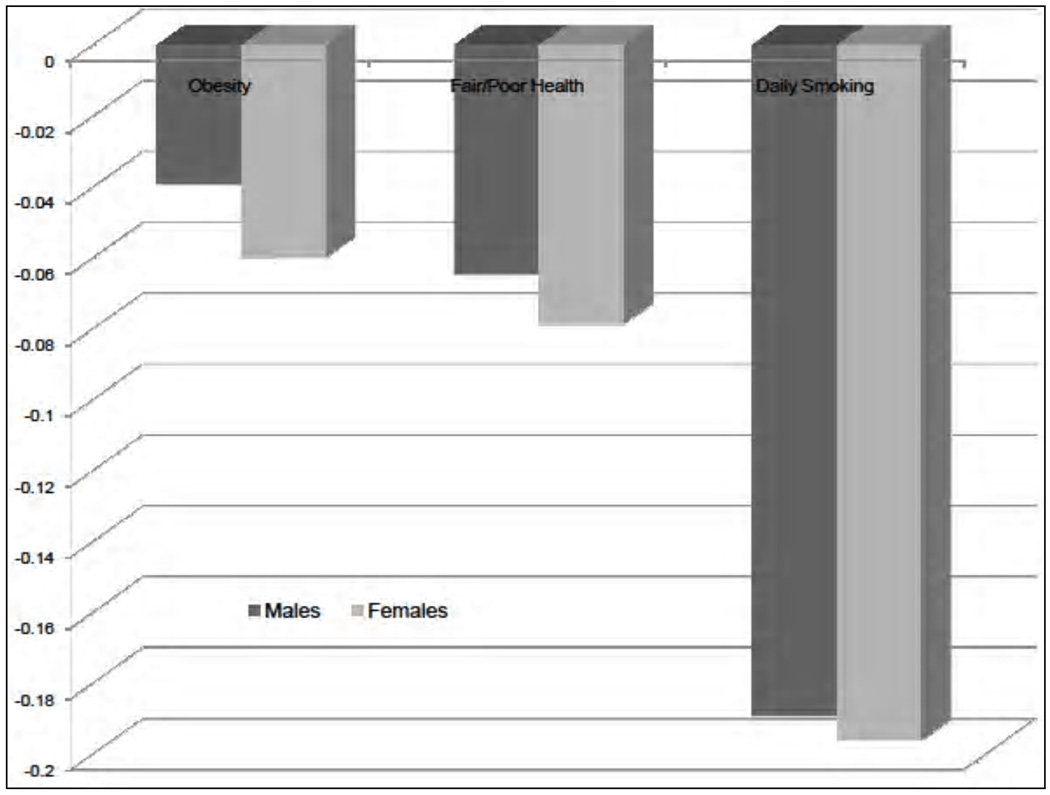
In this article, we discuss only daily smoking, self-reported health and obesity in detail, as these are the three outcomes studied in the health disparities literature more often (see Conti, Heckman, & Urzua, 2010a, 2010b, for a discussion). Summary statistics for our outcome measures are displayed in Table A1 at our Web appendix (http://jenni.uchicago.edu/EdHealth/). Figure 1 displays the full range of educational differentials in our outcome measures. It is interesting to notice that the magnitude of the differential varies depending on the outcome, but a sizeable educational disparity is already present by age 30.

Fig. 1.

Disparities by education. The figure displays the differences in obesity, poor health, and daily smoking by education, between individuals with educational level equal to compulsory education and individuals with some postcompulsory education. The differences are also presented by gender. Adapted from Conti, Heckman, and Urzua (2010a, 2010b).

Measurement System

As indicators of cognitive ability, CHU use the following seven test scores administered to the children at age 10: the Picture Language Comprehension Test, the Friendly Math Test, the Shortened Edinburgh Reading Test, and the four British Ability Scales. CHU use six scales as measurements of noncognitive ability: one administered to the child (the locus of control scale), and five administered to the teacher (perseverance, cooperativeness, completeness, attentiveness, and persistence). As measures of the health endowment, CHU use the height and the head circumference of the child at age 10, and the height of the mother and of the father (also measured when the child was aged 10). Further details are given in the Web appendix, where summary statistics for the measurements are also presented (see Table A2).

Observed Characteristics

CHU include the following set of covariates in both the measurement system and in the outcome equations: mother’s age at birth, mother’s education at birth (whether or not the mother continued education beyond the minimum school-leaving age), father’s social class at birth, total gross family income at age 10, whether the child lived with both parents since birth until age 10, parity, and the number of children in the family at age 10 (CHU also include child’s weight in the measurement equation for child’s height and head circumference, and mother/father weight in the measurement equations for maternal/paternal height). The schooling choice model also includes as a covariate the gender-specific seasonally adjusted rate of unemployment-related benefit claims (the claimant count) as observed in January 1986. Summary statistics for the covariates are presented in Table A3 in our Web appendix.

Distributional Assumption and Estimation Strategy

CHU use mixture of normal approximations to the underlying factors’ distribution. Normal mixtures can flexibly approximate a variety of distributions (see Ferguson, 1983):

$$\left[\begin{array}{c}\hfill {\theta }_C\hfill \\ \hfill {\theta }_N\hfill \\ \hfill {\theta }_H\hfill \end{array}\right]~p_1\mathrm{\Phi }({\mathbf{\mu }}_1,{\mathbf{\Sigma }}_1)+(1-p_1)\mathrm{\Phi }({\mathbf{\mu }}_2,{\mathbf{\Sigma }}_2)$$

where μ₁ and μ₂ are vectors of dimension 3 × 1 and Σ₁ and Σ₂ are matrices of dimension 3 × 3. The variance–covariance matrices are not restricted to be diagonal matrices, so the underlying factors are allowed to be correlated.

For the idiosyncratic components associated with the binary choice models (υ_V, υ_ε0, υ_ε1), CHU assume independent normal distributions with a mean of 0 and a variance of 1. For the idiosyncratic components associated with the continuous outcomes (υ_U0, υ_U1), CHU assume independent normal distributions with means equal to zero and unknown variances.

The joint density of the outcomes conditional on observables is as follows:

$$f(Y,B,D,M_C,M_N,M_H|X,Z,Q)$$

where f(·) is the joint density of continuous (Y) and discrete outcomes (B), schooling choices (D), cognitive measures (M_C), noncognitive scales (M_N), and early health variables (M_H). Written in terms of unobservables, the density is as follows:

$${\displaystyle {\iiint }_{({\theta }_C,{\theta }_N,{\theta }_H)\in \mathrm{\Theta }}f(Y,B,D,M_C,M_N,M_H|X,Z,Q,t_C,t_N,t_H)d{F}_{\theta }(t_C,t_N,t_H)}$$

where f(·) is defined as above and F_θ(·) denotes the joint cumulative density associated with unobserved cognitive (θ_C), noncognitive (θ_N) and health (θ_H) endowments. Notice that, conditional on unobserved factors (and observed characteristics), the components of D, M_C, M_N, and M_H are independent, and the sample likelihood simplifies accordingly. (Y and B are not independent of D given X (see Equations 4 and 5). However, conditional on θ, any effect of D on Y and B is causal). Using latent factors to account for the correlation across outcomes, schooling decisions, and measurements simplifies the computation. CHU use Bayesian Markov Chain Monte Carlo methods to compute the sample likelihood. See CHU for further details.

Defining the Causal Effects of Interventions

Δ_i = Y_i1 − Y_i0 denotes the person-specific treatment effect for a given individual i and outcome Y. As before, Y_i1 and Y_i0 denote the outcomes associated with postcompulsory education (D_i = 1) and compulsory education (D_i = 0), respectively. We illustrate how to use our framework to compute treatment parameters in the context of a single outcome. However, our discussion directly extends to the more general case of vectors of continuous and discrete outcomes.

Δ_i involves factual and counterfactual outcomes. The counterfactual outcome refers to the same individual—what would the outcome have been had he or she made a different choice?

For a given person we seek to determine what would be his or her outcome if he or she continued education after compulsory schooling compared to the case where they do not. As our model deals with the estimation of counterfactual outcomes, we can use it to estimate the distribution of person-specific treatment effects. With this distribution in hand, we can compute different average treatment parameters. We focus on the average treatment effect in this paper⁷ (i.e., on the average effect of the treatment on a person drawn randomly from the population of individuals):

$${\mathrm{\Delta }}^{ATE}\equiv {\displaystyle \iint E(Y_1-Y_0|X=x,\theta =t)d{F}_{X,\theta }(x,t),}$$

where we integrate E(Y₁ − Y₀|X = x, θ = t) (the average treatment effect given X = x and θ = t) with respect to the distributions of X and θ, where F_X,θ(x, t) is the joint distribution of X and θ evaluated at x, t. (We omit the subindex i for simplicity—Y and X denote any outcome variable and associated covariates).

For the question addressed in this paper, knowledge of the distributional parameters is fundamental. Does anybody benefit from post-compulsory education? Among those who stay on in school after 16, what fraction benefits? The factor structure setup allows us to estimate these distributional parameters, following Aakvik et al. (2005) and Carneiro et al. (2003). We now discuss the empirical results of CHU.

Empirical Results

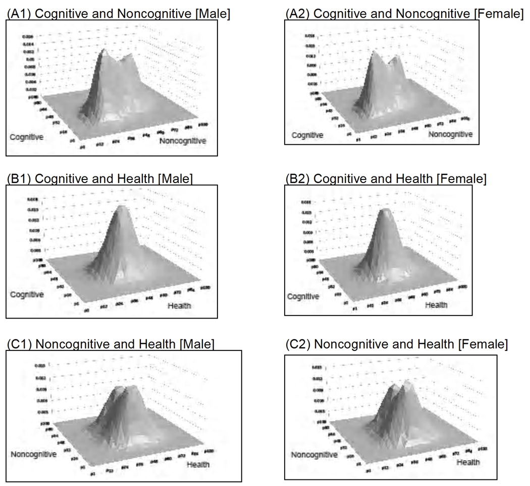
Figure 2 presents the estimated distributions of cognitive, noncognitive, and health endowments for males and females, respectively. Panels A and C in both figures demonstrate the importance of not imposing normal distributions for θ. Furthermore, the comparison between males and females suggest robust patterns, with the cognitive component highly correlated with the noncognitive component for both genders.

Fig. 2.

Joint distributions of the endowments. A: Cognitive and noncognitive endowments in males and females. B: Cognitive and health endowments in males and females. C: Noncognitive and health endowments in males and females. The figures show the joint distributions of cognitive, noncognitive, and health endowments and are generated using simulated data from our model. The simulated data contains the same number of observations as the actual data. The estimated correlations are as follows: cognitive and noncognitive endowments = .544 for males and .541 for females, cognitive and health endowments = .176 for males and .153 for females, and noncognitive and health = .093 for males and .040 for females. Finally, for each endowment, the mean is standardized to be zero. Adapted from Conti, Heckman, and Urzua (2010a, 2010b).

The Role of Early Endowments as Determinants of Adult Outcomes

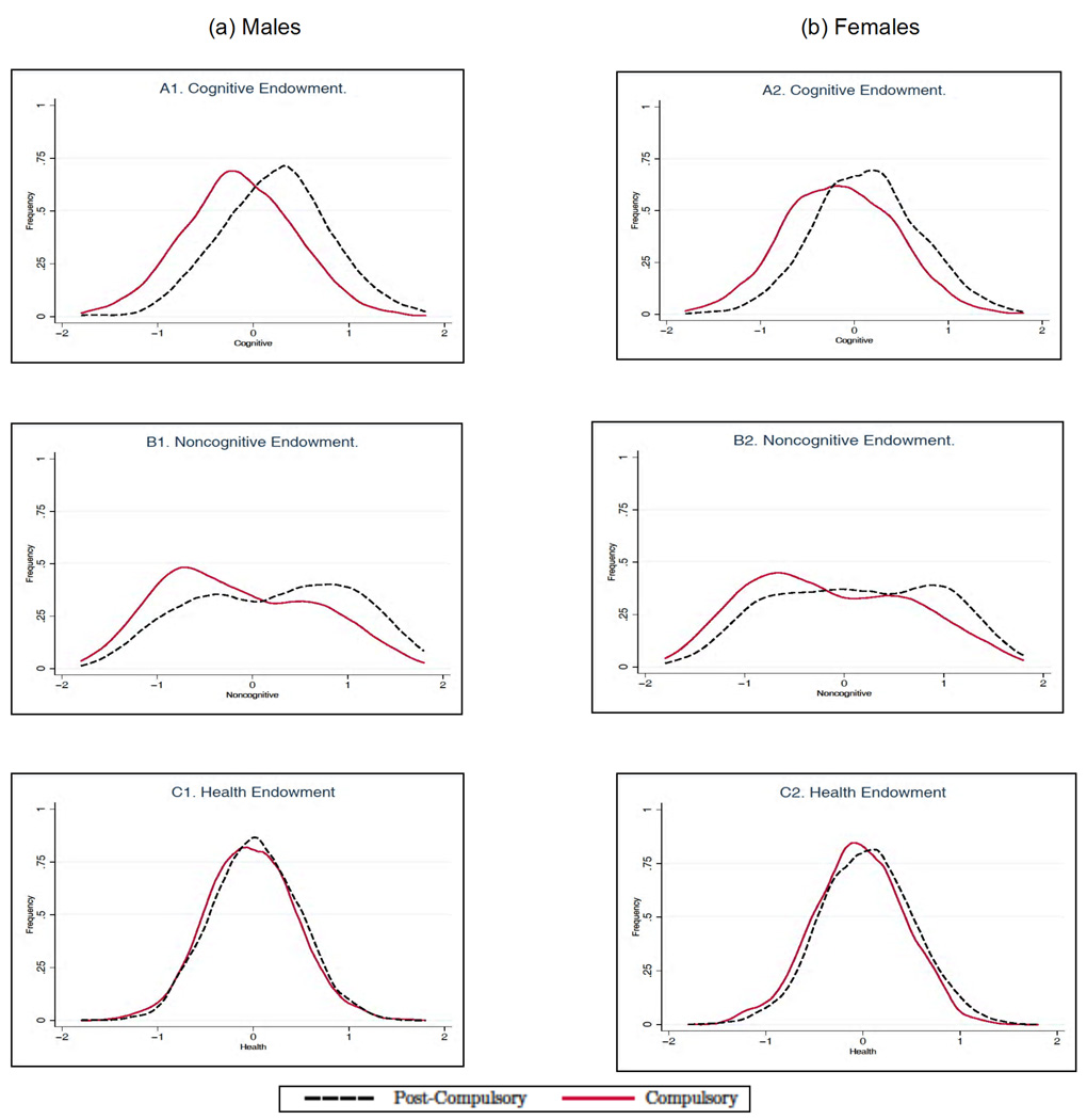
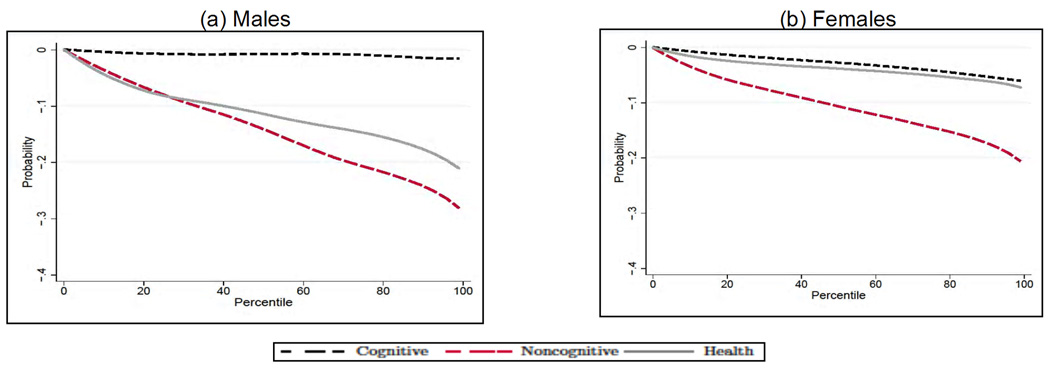
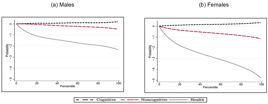
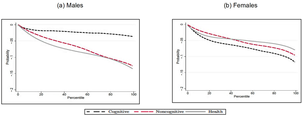
Figure 3 presents the sorting of individuals across schooling levels in terms of the distributions of cognitive, noncognitive, and health endowments. There is a clear sorting of high cognitive and noncognitive individuals into the postcompulsory level of schooling. The pattern is observed for both males and females. The sorting on the health endowment is not as strong as the sorting observed in Panels A1–A2 (cognitive) and B1–B2 (noncognitive), but it is statistically significant for females.⁸ Table 1 reports the marginal effects of θ on daily smoking, obesity, and self-reported health by level of education.⁹ Notice that cognitive ability is a significant determinant of the educational choice, but it basically plays no role on health outcomes (the only exception is the case of poor health for females in the low-education group). On the contrary, noncognitive ability, which is also a significant determinant of the educational choice, exerts a powerful role in reducing the probability of engaging in unhealthy behaviors such as smoking and poor health at age 30 (notice that, in the latter case, the effect of noncognitive ability only achieves statistical significance for the low-education group). We also uncover the role played by early health conditions. For males, early health conditions have no significant effect on the probability of staying on beyond the minimum compulsory level of education, but have a direct effect on all the health outcomes at age 30. For females the effect of health conditions at age 10 seems to work mainly through the educational channel. Notice that, for both males and females, children with a better health endowment at 10 are less likely to be obese by age 30, which is consistent with our modeling of the health factor as a physical health endowment. To gain a better understanding of the overall impact of early life factors, including their effect through education, we compute the predicted unconditional outcome (i.e., the outcome not dependent on education; results by level of education are qualitatively similar; see CHU) and we plot it by percentile of the respective factors in Figures 4–6. In each case, for a given outcome Y, endowment θ_j, and percentile P_θj, we compute E[Y |θ_j ∈ P_θj] by integrating out the observable characteristics and fixing the remaining two unobserved endowments at their overall mean, and we normalize the predicted outcome to zero at the first percentile of the distribution of each factor, so that we can compare the relative magnitude of their effects for both genders.

Fig. 3.

Marginal distributions of endowments for males (A) and females (B) by schooling level. The figures show the marginal distributions of cognitive, noncognitive, and health endowments and are generated using simulated data from our model. The simulated data contains the same number of observations as the actual data. Adapted from Conti, Heckman, and Urzua (2010a, 2010b).

Table 1.

Marginal Effects of Endowments on Outcomes by Educational Level

	Male			Female
Variable	Cognitive	Noncognitive	Health	Cognitive	Noncognitive	Health
Education	0.205 (2.446)	0.045 (2.030)	−0.002 (−0.070)	0.195 (3.732)	0.028 (1.778)	0.047 (1.744)
Daily smoking (C)	0.062 (2.133)	−0.108 (−4.947)	−0.116 (−2.722)	0.017 (0.580)	−0.074 (−3.370)	−0.046 (−1.215)
Daily smoking (PC)	−0.009 (−0.276)	−0.051 (−1.956)	−0.107 (−2.161)	−0.007 (−0.266)	−0.054 (−2.119)	0.005 (0.141)
Poor health (C)	0.017 (0.794)	−0.062 (−2.735)	−0.076 (−1.992)	−0.052 (−1.957)	−0.035 (−1.795)	−0.019 (−0.690)
Poor health (PC)	−0.037 (−1.221)	0.001 (0.062)	−0.076 (−1.599)	−0.017 (−0.700)	−0.025 (−1.254)	−0.038 (−1.142)
Obesity (C)	0.014 (0.688)	−0.026 (−1.515)	−0.108 (−2.195)	−0.012 (−0.407)	−0.028 (−1.334)	−0.210 (−4.000)
Obesity (PC)	−0.007 (−0.251)	0.007 (0.330)	−0.103 (−1.615)	0.039 (1.160)	−0.037 (−1.491)	−0.268 (−3.741)

Note. Adapted from Conti, Heckman, and Urzua (2010a, 2010b). Marginal effects are defined as the analytical derivative averaged over the unconditional distribution of X and θ: ${\displaystyle \iint \frac{\delta \text{Pr}(y_k=1|X,\theta )}{\delta {\theta }_j}d{F}_{X,\theta }}$, with k = {0,1} (k = 0 if the person has stopped at the compulsory level of education, k = 1 if the person has continued beyond the compulsory level) and j = {C, N, H}. Numbers in parentheses are t statistics. C = compulsory; PC = postcompulsory.

Fig. 4.

Effects of endowments on daily smoking outcomes for males (A) and females (B). The endowments and the outcomes are simulated from the estimates of the model in each panel; when we compute the effect of each endowment on the outcome, we integrate out the observable characteristics and fix the other two endowments at their overall mean. Adapted from Conti, Heckman, and Urzua (2010a, 2010b).

Fig. 6.

Effects of endowments on obesity outcomes for males (A) and females (B). The endowments and the outcomes are simulated from the estimates of the model in each panel; when we compute the effect of each endowment on the outcome, we integrate out the observable characteristics and fix the other two endowments at their overall mean. Adapted from Conti, Heckman, and Urzua (2010a, 2010b).

Our first striking result points to a much lesser role for cognitive ability than has been emphasized in the cognitive epidemiology literature. The result is especially strong for males: A shift from the bottom to the top of the cognitive ability distribution brings about no significant change in the probability of daily smoking (Fig. 4, Panel A), of having poor health (Fig. 5, Panel A), or of being obese (Fig. 6, Panel A) at age 30. The picture is only slightly different for females: cognitive ability also plays no role on the probability of being a daily smoker (Fig. 4, Panel B) or of being obese (Fig. 6, Panel B), but it is an important determinant of the probability of having poor health (Fig. 5, Panel B). The second result that we emphasize is that both noncognitive ability and early health have effects of comparable magnitude. For example, a successful noncognitive/health intervention that would move a child from the bottom to the top percentile of their respective distributions would bring about a reduction in the probability of having poor health at age 30 by more than 10% for males (Fig. 5, Panel A) and by more than 5% for females (Fig. 5, Panel B). The only exception is obesity: for this outcome, the early health endowment is the single major determinant—a finding that corroborates our interpretation of it as physical health.

Fig. 5.

Effects of endowments on fair or poor health outcomes for males (A) and females (B). The endowments and the outcomes are simulated from the estimates of the model in each panel; when we compute the effect of each endowment on the outcome, we integrate out the observable characteristics and fix the other two endowments at their overall mean. Adapted from Conti, Heckman, and Urzua (2010a, 2010b).

Education

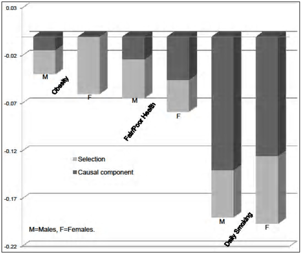
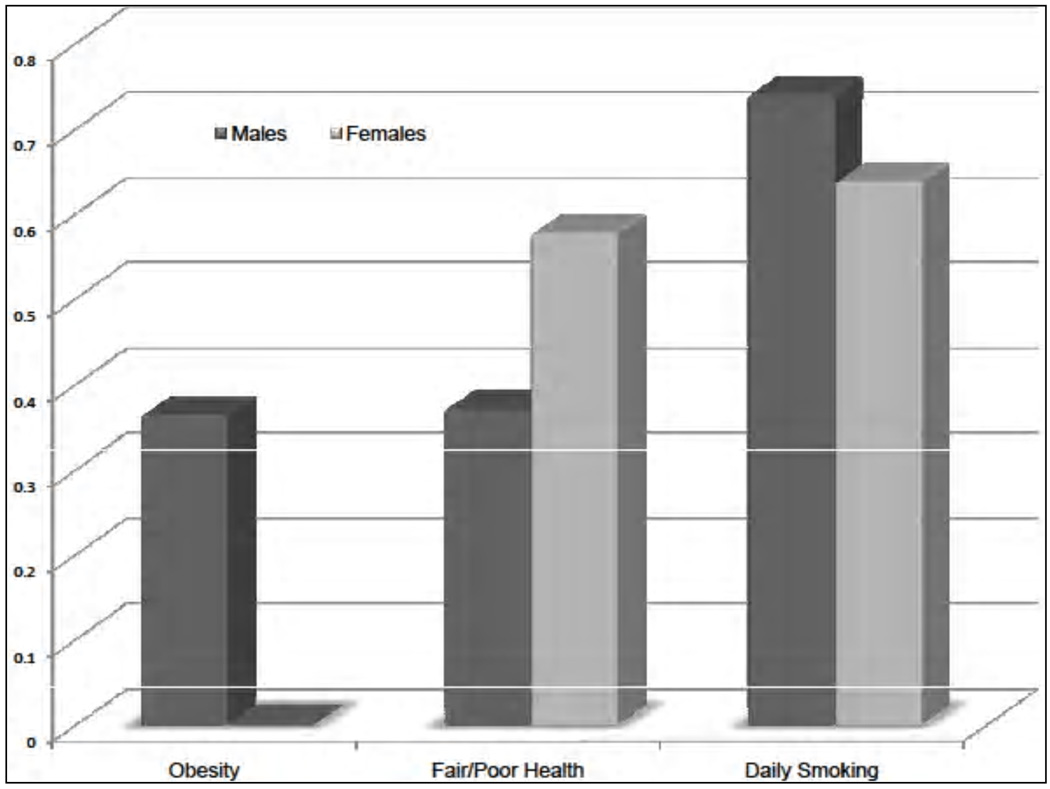
We now analyze the causal effect of education on the outcomes we consider. The results are shown in Figure 7, where the observed disparities are decomposed into the average treatment effect of education (the darker region) and the effect of selection. Notice that education has a causal effect on most outcomes for both males and females. To gain a better understanding of the role played by education in reducing health disparities, we complement Figure 7 with Figure 8, which displays the fraction of the observed differential that can be attributed to education. We see that education plays an important role in explaining differences in smoking behavior, but it accounts for half or less than half of the observed differential in self-reported health. We also uncover significant gender differences: Education plays a much more important role in accounting for the gap in obesity rates for males than it does for females (notice the difference in obesity by education is entirely due to selection for females). This emphasizes the importance of taking the gender dimension into account when studying health disparities.

Fig. 7.

Decomposition of the observed disparities in outcomes by education. The bar heights show the difference in outcomes by educational level (postcompulsory schooling vs. compulsory schooling). The darker region within each bar shows the fraction of the raw gap arising from the causal contribution of education. The rest is due to selection. Adapted from Conti, Heckman, and Urzua (2010a, 2010b).

Fig. 8.

Fraction of the observed disparities in outcomes due to education. The figure displays the fractions of the observed differentials that can be attributed to the effect of education. Specifically, if we denote by Δ the observed differences in outcome Y (i.e. Δ = E[Y₁|D = 1] − E[Y₀|D = 0]), in this figure we present $\frac{E[Y_1-Y_0]}{E[Y_1|D=1]-E[Y_0|D=0]}$. The differential in obesity by education for females is entirely explained by selection. Adapted from Conti, Heckman, and Urzua (2010a, 2010b).

Distribution of Treatment Effects

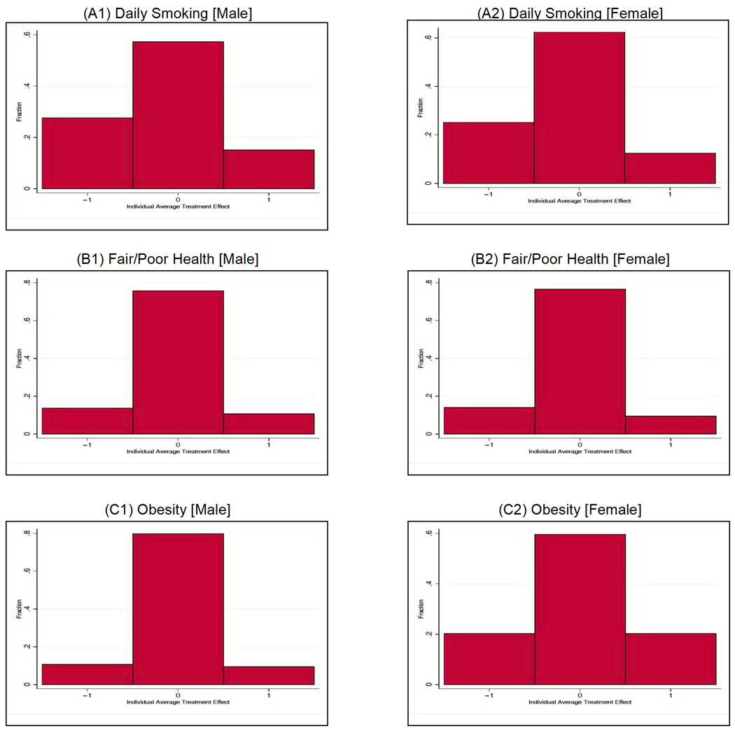
We now move beyond the traditional literature that only considers mean effects and estimate distributions of treatment effects (see Fig. 9). Knowledge of these distributions is fundamental if we want to uncover what lies behind a “zero” average treatment effect and determine the proportion of the individuals who actually benefit from the treatment. We notice that, in the case of smoking, the proportion of people who gain is much bigger than the proportion of people who “lose”,¹⁰ so the average treatment effect turns out to be negative (Fig. 9, Panels A1 and A2). (In each graph, the height of the bar on the left represents the proportion of individuals who would have a successful outcome if treated (i.e., Y₁ = 0) but an unsuccessful outcome if not treated (i.e., Y₀ = 1), so that the average treatment effect for this group is −1. The opposite holds for the bar on the right. The height of the middle bar represents the proportion of individuals who would be unaffected by the treatment.)

Fig. 9.

Population distribution of the average treatment effect. A: Daily smoking (males and females). B: Fair/poor health (males and females). C: Obesity (males and females). The figures display the distribution of the average treatment effect by gender. The outcomes are simulated from the estimates of the model. The simulated data contains the same number of observations as the actual data. Adapted from Conti, Heckman, and Urzua (2010a, 2010b).

However, consider obesity in females (Fig. 9, Panel C2). We can see that underlying an insignificant average treatment effect of education are gains and losses that balance each other out—the same proportion of women (almost 20%) lose and gain from the treatment. Although usually overlooked in traditional studies on the impact of treatments on outcomes, knowledge of these distributional parameters is fundamental to understanding if there is a fraction of individuals who benefit from a particular policy beyond the average treatment effect (see Abbring and Heckman (2007) for a discussion of distributional treatment effects).

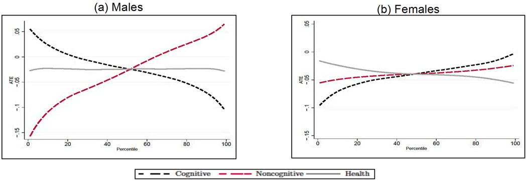
Treatment Effect Heterogeneity: The Role of Early Endowments

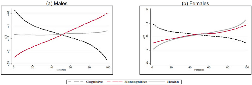
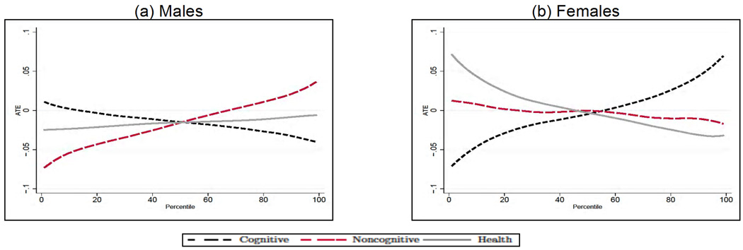
We next analyze how the average treatment effect of education varies along the distribution of cognitive and noncognitive skills, and early health. In each case, for a given outcome Y, endowment θ_j and percentile P_θj, we compute E[Y₁ − Y₀|θ_j ∈ P_θj] by integrating out the observed (by us) characteristics and fixing the remaining two unobserved endowments at their overall mean. Although there is a significant amount of heterogeneity in the effect of education across outcomes by levels of endowments, we can uncover some distinct patterns. First, the beneficial effect of education is much bigger at the top of the cognitive ability distribution for males (see Panel A in Figs. 10–12) and at the bottom for females (apart from smoking, see Panel B in Figs. 10–12). This is particularly interesting in the case of smoking, as it is consistent with the interpretation that the information content on the dangers of smoking provided by postcompulsory education needs to be combined with the capacity to process that information in order to be effective. Second, for all outcomes and genders, education compensates for poor noncognitive ability. Third, there is no heterogeneity in the effect of education for males along the distribution of the health endowment.

Fig. 10.

Treatment effect heterogeneity for daily smoking in males (A) and females (B). The endowments and the outcomes are simulated from the estimates of the model in each panel; when computing the average treatment effect along the distribution of each endowment, we integrate out the observable characteristics and fix the other two endowments at their overall mean. Adapted from Conti, Heckman, and Urzua (2010a, 2010b).

Fig. 12.

Treatment effect heterogeneity for obesity in males (A) and females (B). The endowments and the outcomes are simulated from the estimates of the model in each panel; when computing the average treatment effect along the distribution of each endowment, we integrate out the observable characteristics and fix the other two endowments at their overall mean. Adapted from Conti, Heckman, and Urzua (2010a, 2010b).

The Role of Cognitive Ability

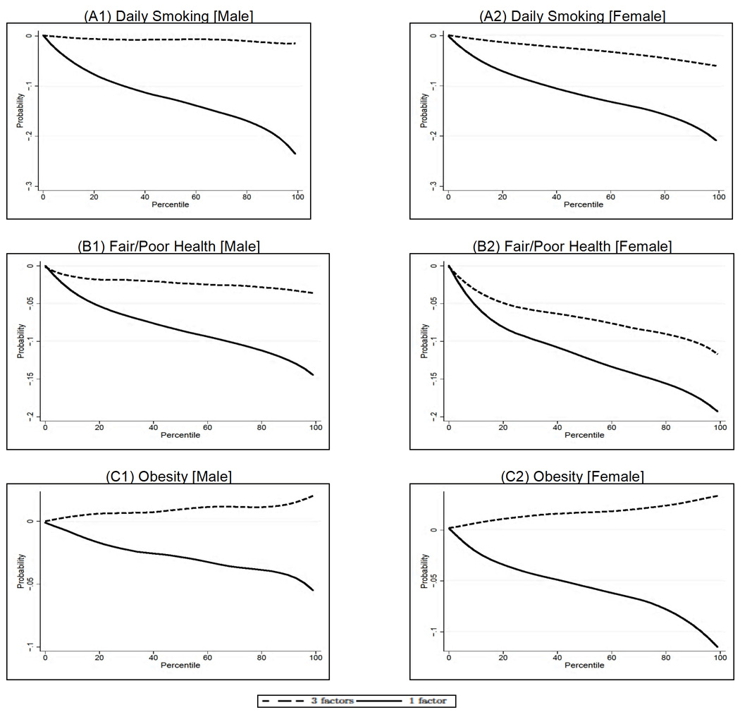
Table 2 compares the effect of cognitive ability in our three-factor model with the effect found in a model where we do not include noncognitive ability and early health. It is striking to note that if early noncognitive traits are not included in the model, early cognitive ability has an important effect for all the outcomes, whereas it plays no role in the model where we consider the three early factors jointly (see for example the smoking and health outcomes). (The same pattern holds when we estimate the effects of the endowments by means of factor scores and simple Probit and OLS regression. The results are available from the authors upon request.) This comes as no surprise if we consider that the estimated correlations between the cognitive and noncognitive endowments are very high (0.54 for both males and females). To better gauge the magnitude of these effects, Figure 13 presents the total effect of cognitive ability on the outcomes in our three-endowment model and in a model without the noncognitive and health endowment. Notice that, in all the cases in which cognitive ability is not a significant determinant of the outcomes in the three-factor model, it has a significant and sizeable impact on them when noncognitive skills and early health are not included; it also has a bigger impact on the probability of being in poor health for females, for which it was a significant determinant in the three-factor model. This serves as a serious caveat for all the work in this area that has not given adequate importance to personality traits and focuses solely on the role played by intelligence early in life (Gale, Batty, & Deary, 2008, and von Stumm, Gale, Batty, & Deary, 2009, acknowledge the relevance of locus of control in the relationship between childhood IQ and adult outcomes).

Table 2.

Marginal Effects of Endowments on Outcomes, by Educational Level: Cognitive Ability Only

	Males		Females
Variable	Three-factor model	Cognitive ability only	Three-factor model	Cognitive ability only
Education	0.205 (2.446)	0.238 (2.524)	0.195 (3.732)	0.220 (3.823)
Daily smoking (C)	0.062 (2.133)	−0.045 (−2.041)	0.017 (0.580)	−0.045 (−1.918)
Daily smoking (PC)	−0.009 (−0.276)	−0.054 (−1.931)	−0.007 (−0.266)	−0.050 (−1.927)
Poor health (C)	0.017 (0.794)	−0.045 (−2.382)	−0.052 (−1.957)	−0.081 (−2.918)
Poor health (PC)	−0.037 (−1.221)	−0.045 (−1.634)	−0.017 (−0.700)	−0.040 (−1.687)
Obesity (C)	0.014 (0.688)	−0.022 (−1.370)	−0.012 (−0.407)	−0.063 (−2.651)
Obesity (PC)	−0.007 (−0.251)	−0.009 (−0.393)	0.039 (1.160)	−0.021 (−0.847)

Note. Adapted from Conti, Heckman, and Urzua (2010a, 2010b). This table displays unstandardized coefficients. The three-factor-model column displays the same results as Table 1 (the "Cognitive" column). The cognitive-ability-only column displays the estimated marginal effects of the cognitive factor on the outcomes for a model that does not include the noncognitive and health factors. Numbers in parentheses are t statistics. C = compulsory; PC = post-compulsory.

Fig. 13.

Effect of cognitive ability. A: Effect on daily smoking for males and females. B: Effect on fair/poor health for males and females. C: Effect on obesity for males and females. The figure shows the effect of cognitive ability on the outcome of interest in the three-factor model versus a model without the noncognitive and health endowments. The dashed line is the same as the one displayed in Figure 4–6 for the cognitive factor in the three-factor model. Adapted from Conti, Heckman, and Urzua (2010a, 2010b).

Possible Applications to Genetic Data

The framework of this article can be applied to the analysis of genetic data. The most obvious way is to include θ_G as an element of θ_t. This approach is somewhat unsatisfactory because θ_Ct, θ_Nt, and θ_Ht likely have genetic components.

One way to address this is through the technology of skill formation (Cunha & Heckman, 2007, 2008, 2009; Cunha, Heckman, & Schennach, 2010). Latent capabilities θ̃_t = (θ_Ct, θ_Nt, θ_Ht) may be produced by investment I_t, which includes parental environments, schooling and the effects of neighborhoods and social environments:

$${\tilde{\theta }}_t=f({\tilde{\theta }}_{t-1},{\theta }_G,I_{t-1})$$ (9)

where θ_G, the genetic factor, affects the acquisition of capabilities. At t = 0, which corresponds to birth, I₋₁ denotes the in-utero conditions (Gluckman & Hanson, 2005, 2006), and θ̃₋₁ = 0. Thus, early life conditions determine lifetime capabilities. θ_GD_i = 1 See Cunha and Heckman (2008) and Cunha, Heckman, and Schennach (2010) for estimates of similar models that show the promise of this approach (though they do not use genetic data).

Notice that we can allow the genetic factor θ_G to affect both the choice of treatment (e.g., whether D_i = 1 or not) and the outcomes given the choices (it is a component of θ in Equations 6, 7, and 8). Hence our model can identify gene–environment correlations (rGE), in which genes determine the selection into environments (the component of α_V corresponding to θ_G is not zero), and gene–environment interactions (G×E), in which environments can modify the association between genes and outcomes (the components of α_U1 and α_U0 corresponding to genes are not zero).

One possible way to use genetic data is as follows. First, our modeling strategy easily accommodates the case in which a single genetic marker proxies a certain genotype, modeling what Reiss and Leve (2007) call “allele–environment” interaction. A second possibility is to capitalize on recent advances in epigenotyping (a method for assaying the methylation status of DNA) and use the proportion of methylation in C-phosphate-G sites (cytosine and guanine separated by a phosphate that links the two together in the DNA sequence) as measurements. In this case, our modeling strategy would naturally extend to a dynamic setting, to allow for the fact that methylation patterns can change over time, and θ_Gt would be the methylated gene, which is what affects choices of environments and outcomes (see Schneider et al., 2010—we plan to extend our approach to a dynamic setting along the lines of Cunha & Heckman, 2008, Cunha et al., 2010, and Heckman, 2007). A third possibility is to use genome-wide expression data from DNA microarray. In these latter cases, clustering would naturally arise according to similarity in patterns of gene expression (see Eisen, Spellman, Brown, & Botstein, 1998), and our framework would allow us to analyze significant differential expression after a given treatment. In addition to this, the availability of the three different types of data would allow us to examine the extent to which the genotype affects both gene expression and DNA methylation (see Gibbs et al., 2010, for a very recent analysis along these lines). Clearly, one advantage of modeling the second or third type of data relies on the fact that changes in methylation patterns and gene expression reflect genome-wide activity, whereas we would use the first type of data to analyze the effect that specific alleles have on the choice of environments and on the outcomes.

Notice that each of the four endowments can be itself a vector: this would allow us to model, respectively, fluid and crystallized intelligence, the Big Five, physical and mental health, and, in the case of θ_G, gene–gene interactions (G×G), which, if not properly accounted for, can give rise to false gene-environment correlations (rGE). Finally, it is worth remarking that as our model allows each endowment to have an effect on the choice of environment and on a variety of outcomes, it encompasses pleiotropy (i.e., the cases in which genes have differential effects on more than one phenotype).

Twin Data

If analysts have access to twin data, they do not need direct measurements on genetic markers. In contrast to the approach previously discussed, we now deal with the case of observed environments but with no direct proxy for genotype. The availability of data on twins allows us to estimate genetic effects even in absence of measures of genotypes.

Traditionally, twin studies decompose the phenotypic variance into three components: additive genetic, common environment, and unique environment—the so-called ACE model. Here, we discuss a binary environment, and we refer the reader to recent work by Purcell (2002) and Rathouz, Van Hulle, Rodgers, Waldman, and Lahey (2008) for the case of continuous moderators. For the binary environment, Eaves (1982) proposed a simple method for detecting G×E: estimate components of phenotypic variance conditional on environmental exposure, such that, if the amount of variance explained by genetic factors differs between exposed and unexposed twins, then this will constitute evidence for G×E (as a different environment is applied over the same set of genotypes). Eaves (1982) recognized that phenotypic differences might be also due to active gene–environment correlations but did not propose a method to separate out the two components. Our method encompasses both rGE and G×E with twins data in the context of the genetic factor model proposed by Martin and Eaves (1977).

As the choice and the outcome portions of our model are unchanged (apart from the presence of a set of outcomes and a choice equation for each twin), we focus on the measurement system to show how genetic effects can be identified from multiple proxies on the same factor for MZ and DZ twins. M_ij is defined as the ith measurement M on twin j (think of M as a test of cognitive ability, for example). Let us further assume that we have two measurements for each twin, and that each measurement is a linear function of the factor it is designed to proxy (cognitive ability, in the context of the above example) and of the genetic endowment. Thus, we relax the assumption of dedicated measurements. Defining ${\theta }_1^{*}$ as the cognitive ability of Twin 1 and ${\theta }_2^{*}$ as the cognitive ability of Twin 2, we leave the conditioning on X implicit to simplify the exposition and write the measurement system as follows:

$$\begin{array}{c}\hfill M_{11}={\theta }_1^{*}+{\beta }_1{\theta }_{G1}+{\upsilon }_{11}\hfill \\ \hfill M_{21}={\alpha }_{21}{\theta }_1+{\beta }_2{\theta }_{G1}+{\upsilon }_{21}\hfill \\ \hfill M_{12}={\theta }_2^{*}+{\beta }_1{\theta }_{G2}+{\upsilon }_{12}\hfill \\ \hfill M_{22}={\alpha }_{22}{\theta }_2+{\beta }_2{\theta }_{G2}+{\upsilon }_{22}\hfill \end{array}$$

where we make the standard assumptions in twin design that (β₁, β₂) are the same for both twins, and we use the first measurement for each twin to normalize the factor ${\theta }_j^{*}$. In addition, we assume that ${\sigma }_{{\theta }_1^{*}}^2={\sigma }_{{\theta }_2^{*}}^2$. Let us further assume for the moment ${\theta }_j^{*}╨{\theta }_G$, where “╨” denotes independence. By using the fact that cov(θ_G1, θ_G2) = 1 in the case of MZ twins, and cov(θ_G1, θ_G2) = 0.5 in the case of DZ twins, we obtain the following covariances:

$$\text{MZ Twins}\{\begin{array}{cc}\mathit{\text{cov}}(M_{11},M_{21})=\hfill & \hfill {\alpha }_{21}{\sigma }_{{\theta }_1^{*}}^2+{\beta }_1{\beta }_2\hfill \\ \mathit{\text{cov}}(M_{12},M_{22})=\hfill & \hfill {\alpha }_{22}{\sigma }_{{\theta }_2^{*}}^2+{\beta }_1{\beta }_2\hfill \\ \mathit{\text{cov}}(M_{11},M_{12})=\hfill & \hfill {\sigma }_{{\theta }_1^{*}{\theta }_2^{*}}+{\beta }_1^2\hfill \\ \mathit{\text{cov}}(M_{21},M_{22})=\hfill & \hfill {\alpha }_{21}{\alpha }_{22}{\sigma }_{{\theta }_1^{*}{\theta }_2^{*}}+{\beta }_2^2\hfill \end{array}$$

$$\text{DZ Twins}\{\begin{array}{cc}\mathit{\text{cov}}(M_{11},M_{21})=\hfill & \hfill {\alpha }_{21}{\sigma }_{{\theta }_1^{*}}^2+0.5{\beta }_1{\beta }_2\hfill \\ \mathit{\text{cov}}(M_{12},M_{22})=\hfill & \hfill {\alpha }_{22}{\sigma }_{{\theta }_2^{*}}^2+0.5{\beta }_1{\beta }_2\hfill \\ \mathit{\text{cov}}(M_{11},M_{12})=\hfill & \hfill {\sigma }_{{\theta }_1^{*}{\theta }_2^{*}}+0.5{\beta }_1^2\hfill \\ \mathit{\text{cov}}(M_{21},M_{22})=\hfill & \hfill {\alpha }_{21}{\alpha }_{22}{\sigma }_{{\theta }_1^{*}{\theta }_2^{*}}+0.5{\beta }_2^2\hfill \end{array}$$

From the eight covariances and the assumption that ${\sigma }_{{\theta }_1^{*}}^2={\sigma }_{{\theta }_2^{*}}^2$, we are generally able to identify all the seven parameters of the measurement system $({\beta }_1,{\beta }_2,{\alpha }_{21},{\alpha }_{22},{\sigma }_{{\theta }_1^{*}}^2={\sigma }_{{\theta }_2^{*}}^2,{\sigma }_{{\theta }_1^{*}{\theta }_2^{*}})$ with (β₁, β₂) and (α₂₁, α₂₂) identified up to sign. With this type of information, we can relax the assumption that ${\theta }_j^{*}╨{\theta }_G$, and identify ${\sigma }_{{\theta }_j^{*}{\theta }_G}$, at the cost of imposing an assumption like ${\sigma }_{{\theta }_1^{*}{\theta }_G}={\sigma }_{{\theta }_2^{*}{\theta }_G}$. Clearly, the availability of a number of measurements (>2) for each twin, or of multiple time periods, would allow us also to relax this equicorrelation assumption and to identify richer models. The development of these models is left for another occasion.

Adoption Data

The model can be applied to adoption data. As in the case of twins data, one defining characteristic of the adoption design is the possibility of identifying and estimating genetic effects in the absence of direct measurements on genotypes. In the following analysis, we present the simplest possible model that allows us to exploit adoption data (our model currently does not consider the case of adoption of relatives—this is a straightforward extension that is left for a future occasion). For ease of exposition, we present this model in the context of a specific application on structured parenting (D, the environment) and child psychopathology (Y, the outcome; see Leve et al., 2009, for the original application). Define θ_B as the birth parents (BP) factor (e.g. depression), θ_A as the adoptive parents (AP) factor (same personality disfunction as for the BP), and θ_C as the adopted child (AC) factor (e.g., behavioral problems as early precursors of psychopathology). By defining the treatment as structured parenting and the outcome as child psychopathology, we notice that we are able to model genetic and environmental effects on parenting, while allowing at the same time parenting to exert a differential effect on child psychopathology as a function of genetic endowments. Thus, we incorporate both rGE and G×E in this setup. We rewrite our choice equation as follows:

$$S^{*}=\gamma Z+{\alpha }_{BV}{\theta }_B+{\alpha }_{AV}{\theta }_A+{\alpha }_{CV}{\theta }_C+{\upsilon }_V$$ (10)

and we rewrite the potential outcome (child psychopathology) associated with exposure to structured parenting as follows:

$$Y_1={\mu }_1(X)+{\alpha }_{B1}{\theta }_B+{\alpha }_{A1}{\theta }_A+{\alpha }_{C1}{\theta }_C+{\upsilon }_{U1}$$ (11)

and the potential outcome obtained if the parent does not adopt a structured parenting approach is as follows:

$$Y_0={\mu }_0(X)+{\alpha }_{B0}{\theta }_B+{\alpha }_{A0}{\theta }_A+{\alpha }_{C0}{\theta }_C+{\upsilon }_{U0}$$ (12)

It is now instructive to interpret each of the model parameters: α_BV represents evocative rGE, α_B1 and α_B0 capture how parenting moderates genetic risk, α_AV captures the indirect effect of adoptive parents personality through parenting, α_A1 and α_A0 capture the direct effect on the child psychopathology, α_CV captures the direct effect of child’s early behavioral problems on parenting, and α_C1 and α_C0 allow parenting to have a differential effect on child’s outcomes depending on child’s early behavioral problems. It turns out that the covariances among the factors have a meaningful interpretation in this setting: cov(θ_A, θ_B) captures the presence of selective placement or adoption openness, cov(θ_A, θ_C) captures the similarity between adoptive parents and children that reflects environmental influences, and cov(θ_B, θ_C)captures the similarity between birth parents and children that reflect genetic influences. Under general conditions specified in Carneiro et al. (2003) and Abbring and Heckman (2007), the model is identified. We hope to apply these models in future work.

Conclusions

In this article, we apply a general model for causal inference of interventions (choices of environments) in the presence of latent variables that affect choices of interventions and outcomes to disentangle the causal effect of interventions from the role played by latent factors as they determine outcomes. In an empirical illustration of our methodology, we draw on the work of Conti, Heckman, and Urzua (2010a, 2010b) that determines the role played by cognitive, noncognitive, and early health endowments on adult outcomes. We identify the causal effect of education on health and health-related behaviors. We develop an empirical model of schooling choice and postschooling outcomes, in which both dimensions are influenced by latent factors (cognitive, noncognitive, and health). We show that family background characteristics and cognitive, noncognitive, and health endowments present as early as age 10 are important determinants of disparities in smoking rates, poor health, and obesity at age 30. We show that not properly accounting for personality traits overestimates the importance of cognitive ability in determining later health. We show that selection explains more than half of the observed difference by education in poor health and obesity, and that education has an important causal effect in explaining differences in smoking rates. We uncover significant gender differences. We go beyond the current literature, which usually estimates mean effects to compute distributions of treatment effects. We show how the health returns to education can vary also among individuals who are similar under their observed characteristics and how a mean effect can hide gains and losses for different individuals. This highlights the crucial role played by the early years in promoting health and the importance of prevention in the reduction of health disparities. We have discussed how the method can be applied to analyze how genes affect the choice of interventions (environments) and the potential outcomes resulting from interventions. An empirical application of the model to genetic data is left to the future.

Fig. 11.

Treatment effect heterogeneity for fair/poor health in males (A) and females (B). The endowments and the outcomes are simulated from the estimates of the model in each panel; when computing the average treatment effect along the distribution of each endowment, we integrate out the observable characteristics and fix the other two endowments at their overall mean. Adapted from Conti, Heckman, and Urzua (2010a, 2010b).

References

- Aakvik A, Heckman JJ, Vytlacil EJ. Estimating treatment effects for discrete outcomes when responses to treatment vary: An application to Norwegian vocational rehabilitation programs. Journal of Econometrics. 2005;125:15–51. [Google Scholar]
- Abbring JH, Heckman JJ. Econometric evaluation of social programs: Part 3. Distributional treatment effects, dynamic treatment effects, dynamic discrete choice, and general equilibrium policy evaluation. In: Heckman J, Leamer E, editors. Handbook of Econometrics. Volume 6B. Amsterdam: Elsevier; 2007. pp. 5145–5303. [Google Scholar]
- Auld MC, Sidhu N. Schooling, cognitive ability and health. Health Economics. 2005;14:1019–1034. doi: 10.1002/hec.1050. [DOI] [PubMed] [Google Scholar]
- Bakermans-Kranenburg MJ, Van Ijzendoorn MH, Pijlman FTA, Mesman J, Juffer F. Experimental evidence for differential susceptibility: Dopamine D4 receptor polymorphism (DRD4 VNTR) moderates intervention effects on toddlers’ externalizing behavior in a randomized controlled trial. Developmental Psychology. 2008;44:293–300. doi: 10.1037/0012-1649.44.1.293. [DOI] [PubMed] [Google Scholar]
- Bamshad M. Genetic influences on health: Does race matter? Journal of the American Medical Association. 2005;294:937–946. doi: 10.1001/jama.294.8.937. [DOI] [PubMed] [Google Scholar]
- Batty GD, Deary IJ, Schoon I, Gale CR. Mental ability across childhood in relation to risk factors for premature mortality in adult life: The 1970 British Cohort Study. Journal of Epidemiology and Community Health. 2007;61:997–1003. doi: 10.1136/jech.2006.054494. [DOI] [PMC free article] [PubMed] [Google Scholar]
- Bauer L, Covault J, Harel O, Das S, Gelernter J, Anton R, Kranzler H. Variation in GABRA2 predicts drinking behavior in project MATCH subjects. Alcoholism: Clinical and Experimental Research. 2007;31:1780–1787. doi: 10.1111/j.1530-0277.2007.00517.x. [DOI] [PMC free article] [PubMed] [Google Scholar]
- Brody G, Beach S, Philibert R, Chen Y, Murry V. Prevention effects moderate the association of 5-HTTLPR and youth risk behavior initiation: Gene × Environment hypotheses tested via a randomized prevention design. Child Development. 2009;80:645–661. doi: 10.1111/j.1467-8624.2009.01288.x. [DOI] [PubMed] [Google Scholar]
- Carneiro P, Hansen K, Heckman JJ. Estimating distributions of treatment effects with an application to the returns to schooling and measurement of the effects of uncertainty on college choice. International Economic Review. 2003;44:361–422. [Google Scholar]
- Case A, Fertig A, Paxson C. The lasting impact of childhood health and circumstance. Journal of Health Economics. 2005;24:365–389. doi: 10.1016/j.jhealeco.2004.09.008. [DOI] [PubMed] [Google Scholar]
- Case A, Lubotsky D, Paxson C. Economic status and health in childhood: The origins of the gradient. American Economic Review. 2002;92:1308–1334. doi: 10.1257/000282802762024520. [DOI] [PubMed] [Google Scholar]
- Commission on Social Determinants of Health. Closing the gap in a generation: Health equity through action on the social determinants of health. Geneva, Switzerland: World Health Organization; 2008. [DOI] [PubMed] [Google Scholar]
- Conti G, Heckman JJ, Lopes H, Piatek R. Constructing economically justified aggregates: An application to the early origins of health. University of Chicago; 2010. Unpublished manuscript. [Google Scholar]
- Conti G, Heckman JJ, Urzua S. Early endowments, education, and health. University of Chicago; 2010a. Unpublished manuscript. [Google Scholar]
- Conti G, Heckman JJ, Urzua S. The education-health gradient. American Economic Review: Papers & Proceedings. 2010b;100:234–238. doi: 10.1257/aer.100.2.234. [DOI] [PMC free article] [PubMed] [Google Scholar]
- Cox DR. Planning of experiments. New York: Wiley; 1958. [Google Scholar]
- Cunha F, Heckman JJ. The technology of skill formation. American Economic Review. 2007;97:31–47. [Google Scholar]
- Cunha F, Heckman JJ. Formulating, identifying and estimating the technology of cognitive and noncognitive skill formation. Journal of Human Resources. 2008;43:738–782. doi: 10.3982/ECTA6551. [DOI] [PMC free article] [PubMed] [Google Scholar]
- Cunha F, Heckman JJ. The economics and psychology of inequality and human development. Journal of the European Economic Association. 2009;7:320–364. doi: 10.1162/jeea.2009.7.2-3.320. [DOI] [PMC free article] [PubMed] [Google Scholar]
- Cunha F, Heckman JJ, Lochner LJ, Masterov DV. Interpreting the evidence on life cycle skill formation. In: Hanushek EA, Welch F, editors. Handbook of the economics of education. Amsterdam: North-Holland; 2006. pp. 697–812. [Google Scholar]
- Cunha FJ, Heckman J, Schennach SM. Estimating the technology of cognitive and noncognitive skill formation. Econometrica. 2010;78:883–931. doi: 10.3982/ECTA6551. [DOI] [PMC free article] [PubMed] [Google Scholar]
- Currie J. Healthy, wealthy, and wise: Socioeconomic status, poor health in childhood, and human capital development. Journal of Economic Literature. 2009a;47:87–122. [Google Scholar]
- Currie J. Policy interventions to address child health disparities: moving beyond health insurance. Pediatrics. 2009b;124 Suppl.:S246–S254. doi: 10.1542/peds.2009-1100M. [DOI] [PubMed] [Google Scholar]
- Currie J, Moretti E. Mother’s education and the intergenerational transmission of human capital: Evidence from college openings. Quarterly Journal of Economics. 2003;118:1495–1532. [Google Scholar]
- Cutler D, Lleras-Muney A. Understanding differences in health behaviors by education. Journal of Health Economics. 2010;29:1–28. doi: 10.1016/j.jhealeco.2009.10.003. [DOI] [PMC free article] [PubMed] [Google Scholar]
- Dahly DL, Adair LS, Bollen KA. A structural equation model of the developmental origins of blood pressure. International Journal of Epidemiology. 2008;37:1–11. doi: 10.1093/ije/dyn242. [DOI] [PMC free article] [PubMed] [Google Scholar]
- Davey Smith G. Health inequalities: Lifecourse approaches. Bristol, United Kingdom: Policy Press; 2003. [Google Scholar]
- Eaves L. The utility of twins. In: Anderson VE, Hauser WA, Penry JK, Sing CF, editors. Genetic basis of the epilepsies. New York: Raven Press; 1982. pp. 249–276. [Google Scholar]
- Eisen M, Spellman P, Brown P, Botstein D. Cluster analysis and display of genome-wide expression patterns. Proceedings of the National Academy of Sciences, USA. 1998;95:14863. doi: 10.1073/pnas.95.25.14863. [DOI] [PMC free article] [PubMed] [Google Scholar]
- Elias JJ. The effects of ability and family background on nonmonetary returns to education. Unpublished doctoral thesis. University of Chicago; 2005. [Google Scholar]
- Ferguson TS. Bayesian density estimation by mixtures of normal distributions. In: Chernoff H, Rizvi M, Rustagi J, Siegmund D, editors. Recent advances in statistics: Papers in honor of Herman Chernoff on his 60th birthday. New York: Academic Press; 1983. pp. 287–302. [Google Scholar]
- Fine MJ, Ibrahim SA, Thomas SB. The role of race and genetics in health disparities research. American Journal of Public Health. 2005;95:2125–2128. doi: 10.2105/AJPH.2005.076588. [DOI] [PMC free article] [PubMed] [Google Scholar]
- Fisher RA. The design of experiments. London: Oliver and Boyd; 1935. [Google Scholar]
- Fuchs VR. Time preference and health: An exploratory study. In: Fuchs VR, editor. Economic aspects of health. Chicago: University of Chicago Press; 1982. pp. 93–120. [Google Scholar]
- Gale CR, Batty GD, Deary IJ. Locus of control at age 10 years and health outcomes and behaviors at age 30 years: The 1970 British Cohort Study. Psychosomatic Medicine. 2008;70:397–403. doi: 10.1097/PSY.0b013e31816a719e. [DOI] [PubMed] [Google Scholar]
- Gibbs JR, van der Brug MP, Hernandez DG, Traynor BJ, Nalls MA, Lai S-L, et al. Abundant quantitative trait loci exist for DNA methylation and gene expression in human brain. Public Library of Science: Genetics, 6. 2010 doi: 10.1371/journal.pgen.1000952. Retrieved from http://www.ncbi.nlm.nih.gov/pmc/articles/PMC2869317/ [DOI] [PMC free article] [PubMed]
- Gluckman PD, Hanson M. The fetal matrix: Evolution, development, and disease. Cambridge, United Kingdom: Cambridge University Press; 2005. [Google Scholar]
- Gluckman PD, Hanson MA. Developmental origins of health and disease. Cambridge, United Kingdom: Cambridge University Press; 2006. [Google Scholar]
- Gottfredson LS, Deary IJ. Intelligence predicts health and longevity, but why? Current Directions in Psychological Science. 2004;13:1–4. [Google Scholar]
- Grossman M. On the concept of health capital and the demand for health. Journal of Political Economy. 1972;80:223–255. [Google Scholar]
- Grossman M. The correlation between health and schooling. In: Terleckyj NE, editor. Household production and consumption. New York: Columbia University Press; 1975. pp. 147–211. [Google Scholar]
- Grossman M. The human capital model. In: Culyer AJ, Newhouse JP, editors. Handbook of health economics. Vol. 1. Amsterdam: Elsevier; 2000. pp. 347–408. [Google Scholar]
- Grossman M. Education and nonmarket outcomes. In: Hanushek E, Welch F, editors. Handbook of the economics of education. Vol. 1. Amsterdam: Elsevier; 2006. pp. 577–633. [Google Scholar]
- Grossman M. The relationship between health and schooling: Presidential address. Eastern Economic Journal. 2008;34:281–292. [Google Scholar]
- Grossman M, Kaestner R. Effects of education on health. In: Behrman JR, Stacey N, editors. The social benefits of education. Ann Arbor, MI: University of Michigan Press; 1997. pp. 69–124. [Google Scholar]
- Hampson SE, Friedman HS. Personality and health: A lifespan perspective. In: John OP, Robins R, Pervin L, editors. The handbook of personality: Theory and research. 3rd ed. New York: Guilford; 2008. pp. 770–794. [Google Scholar]
- Hansen KT, Heckman JJ, Mullen KJ. The effect of schooling and ability on achievement test scores. Journal of Econometrics. 2004;121:39–98. [Google Scholar]
- Hartog J, Oosterbeek H. Health, wealth and happiness: Why pursue a higher education? Economics of Education Review. 1998;17:245–256. [Google Scholar]
- Heckman JJ. The economics, technology and neuroscience of human capability formation. Proceedings of the National Academy of Sciences, USA. 2007;104:13250–13255. doi: 10.1073/pnas.0701362104. [DOI] [PMC free article] [PubMed] [Google Scholar]
- Heckman JJ. Econometric causality. International Statistical Review. 2008;76:1–27. [Google Scholar]
- Heckman JJ. Building bridges between structural and program evaluation approaches to evaluating policy. Journal of Economic Literature. 2010;48:356–398. doi: 10.1257/jel.48.2.356. [DOI] [PMC free article] [PubMed] [Google Scholar]
- Heckman JJ, Honoré BE. The empirical content of the Roy model. Econometrica. 1990;58:1121–1149. [Google Scholar]
- Heckman JJ, Moon SH, Pinto R, Savelyev PA, Yavitz AQ. Analyzing social experiments as implemented: A reexamination of the evidence from the HighScope Perry Preschool Program. Quantitative Economics. 2010;1:1–46. doi: 10.3982/qe8. [DOI] [PMC free article] [PubMed] [Google Scholar]
- Heckman JJ, Sedlacek GL. Heterogeneity, aggregation, and market wage functions: An empirical model of self-selection in the labor market. Journal of Political Economy. 1985;93:1077–1125. [Google Scholar]
- Heckman JJ, Stixrud J, Urzua S. The effects of cognitive and noncognitive abilities on labor market outcomes and social behavior. Journal of Labor Economics. 2006;24:411–482. [Google Scholar]
- Hu Y, Schennach SM. Instrumental variable treatment of nonclassical measurement error models. Econometrica. 2008;76:195–216. [Google Scholar]
- Kaestner R. Adolescent cognitive and non-cognitive correlates of adult health. Bonn, Germany: National Bureau of Economic Research; 2009. [Google Scholar]
- Knudsen EI, Heckman JJ, Cameron J, Shonkoff JP. Economic, neurobiological, and behavioral perspectives on building America’s future workforce. Proceedings of the National Academy of Sciences, USA. 2006;103:10155–10162. doi: 10.1073/pnas.0600888103. [DOI] [PMC free article] [PubMed] [Google Scholar]
- Kolata G. A surprising secret to a long life: Stay in school. 2007 Retrieved from http://www.nytimes.com/2007/01/03/health/03aging.html.
- Kuh D, Ben-Shlomo Y. A lifecourse approach to adult disease. New York: Oxford University Press; 1997. [Google Scholar]
- Leve L, Harold G, Ge X, Neiderhiser J, Shaw D, Scaramella L, Reiss D. Structured parenting of toddlers at high versus low genetic risk: Two pathways to child problems. Journal of the American Academy of Child and Adolescent Psychiatry. 2009;48:1102. doi: 10.1097/CHI.0b013e3181b8bfc0. [DOI] [PMC free article] [PubMed] [Google Scholar]
- Lleras-Muney A. The relationship between education and adult mortality in the United States. Review of Economic Studies. 2005;72:189–221. [Google Scholar]
- Marmot M. Fair society, Healthy Lives: The Marmot Review. Strategic review of health inequalities in England post-2010. London: University College London; 2010. [Google Scholar]
- Martin N, Eaves L. The genetical analysis of covariance structure. Heredity. 1977;38:79–95. doi: 10.1038/hdy.1977.9. [DOI] [PubMed] [Google Scholar]
- McCormick MC. Issues in measuring child health. Ambulatory Pediatrics. 2008;8:77–84. doi: 10.1016/j.ambp.2007.11.005. [DOI] [PubMed] [Google Scholar]
- Meara ER, Richards S, Cutler DM. The gap gets bigger: Changes in mortality and life expectancy, by education, 1981–2000. Health Affairs. 2008;27:350–360. doi: 10.1377/hlthaff.27.2.350. [DOI] [PMC free article] [PubMed] [Google Scholar]
- Neyman J. Statistical problems in agricultural experiments. Journal of the Royal Statistical Society. 1923;2:107–180. [Google Scholar]
- Nicklas BJ, Mychaleckyj J, Kritchevsky S, Palla S, Lange LA, Lange EM, et al. Physical function and its response to exercise: Associations with cytokine gene variation in older adults with knee osteoarthritis. Journals of Gerontology: Series A. Biological Sciences and Medical Sciences. 2005;60:1292–1298. doi: 10.1093/gerona/60.10.1292. [DOI] [PubMed] [Google Scholar]
- Perri TJ. Health status and schooling decisions of young men. Economics of Education Review. 1984;3:207–213. [Google Scholar]
- Purcell S. Variance components models for gene-environment interaction in twin analysis. Twin Research and Human Genetics. 2002;5:554–571. doi: 10.1375/136905202762342026. [DOI] [PubMed] [Google Scholar]
- Quandt RE. A new approach to estimating switching regressions. Journal of the American Statistical Association. 1972;67:306–310. [Google Scholar]
- Rathouz P, Van Hulle C, Rodgers J, Waldman I, Lahey B. Specification, testing, and interpretation of gene-by-measured-environment interaction models in the presence of gene–environment correlation. Behavior Genetics. 2008;38:301–315. doi: 10.1007/s10519-008-9193-4. [DOI] [PMC free article] [PubMed] [Google Scholar]
- Reiss D, Leve L. Genetic expression outside the skin: Clues to mechanisms of Genotype × Environment interaction. Development and Psychopathology. 2007;19:1005–1027. doi: 10.1017/S0954579407000508. [DOI] [PMC free article] [PubMed] [Google Scholar]
- Roberts BW, Harms P, Smith JL, Wood D, Webb M. Using multiple methods in personality psychology. In: Eid M, Diener E, editors. Handbook of multimethod measurement in psychology. Washington, DC: American Psychological Association; 2006. pp. 321–335. [Google Scholar]
- Roberts BW, Kuncel NR, Shiner RL, Caspi A, Goldberg LR. The power of personality: The comparative validity of personality traits, socioeconomic status, and cognitive ability for predicting important life outcomes. Perspectives in Psychological Science. 2007;2:313–345. doi: 10.1111/j.1745-6916.2007.00047.x. [DOI] [PMC free article] [PubMed] [Google Scholar]
- Roy A. Some thoughts on the distribution of earnings. Oxford Economic Papers. 1951;3:135–146. [Google Scholar]
- Rubin DB. Estimating causal effects of treatments in randomized and nonrandomized studies. Journal of Educational Psychology. 1974;66:688–701. [Google Scholar]
- Rutter M, Tizard J, Whitmore K. Education, health and behaviour. London: Longmans; 1970. [Google Scholar]
- Schneider E, Pliushch G, El Hajj N, Galetzka D, Puhl A, Schorsch M, et al. Spatial, temporal and interindividual epigenetic variation of functionally important DNA methylation patterns. Nucleic Acids Research. 2010;38:3880–3890. doi: 10.1093/nar/gkq126. [DOI] [PMC free article] [PubMed] [Google Scholar]
- Shakotko RA, Edwards LN, Grossman M. An exploration of the dynamic relationship between health and cognitive development in adolescence. Bonn, Germany: National Bureau of Economic Research; 1982. [Google Scholar]
- von Stumm S, Gale CR, Batty GD, Deary IJ. Childhood intelligence, locus of control and behaviour disturbance as determinants of intergenerational social mobility: British Cohort Study 1970. Intelligence. 2009;37:329–340. [Google Scholar]
- Whalley LJ, Deary IJ. Longitudinal cohort study of childhood IQ and survival up to age 76. British Medical Journal. 2001;322:819. doi: 10.1136/bmj.322.7290.819. [DOI] [PMC free article] [PubMed] [Google Scholar]
- Wolfe B. The influence of health on school outcomes: A multivariate approach. Medical Care. 1985;23:1127–1138. doi: 10.1097/00005650-198510000-00001. [DOI] [PubMed] [Google Scholar]
Associated Data
This section collects any data citations, data availability statements, or supplementary materials included in this article.