Social Network Theory Applied to Resting-State fMRI Connectivity Data in the Identification of Epilepsy Networks with Iterative Feature Selection

Abstract

Epilepsy is a brain disorder usually associated with abnormal cortical and/or subcortical functional networks. Exploration of the abnormal network properties and localization of the brain regions involved in human epilepsy networks are critical for both the understanding of the epilepsy networks and planning therapeutic strategies. Currently, most localization of seizure networks come from ictal EEG observations. Functional MRI provides high spatial resolution together with more complete anatomical coverage compared with EEG and may have advantages if it can be used to identify the network(s) associated with seizure onset and propagation. Epilepsy networks are believed to be present with detectable abnormal signatures even during the interictal state. In this study, epilepsy networks were investigated using resting-state fMRI acquired with the subjects in the interictal state. We tested the hypothesis that social network theory applied to resting-state fMRI data could reveal abnormal network properties at the group level. Using network data as input to a classification algorithm allowed separation of medial temporal lobe epilepsy (MTLE) patients from normal control subjects indicating the potential value of such network analyses in epilepsy. Five local network properties obtained from 36 anatomically defined ROIs were input as features to the classifier. An iterative feature selection strategy based on the classification efficiency that can avoid ‘over-fitting’ is proposed to further improve the classification accuracy. An average sensitivity of 77.2% and specificity of 83.86% were achieved via ‘leave one out’ cross validation. This finding of significantly abnormal network properties in group level data confirmed our initial hypothesis and provides motivation for further investigation of the epilepsy process at the network level.

1. Introduction

Epilepsy is a common brain disorder characterized by recurrent unprovoked seizures, associated with functionally abnormal, distributed cortical and subcortical network(s). The investigation of abnormal functional network properties and localization of the brain regions responsible for seizure generation and propagation are key issues for both understanding the epilepsy networks and potentially guiding therapeutic strategies.

The evidence for human epilepsy networks comes mostly from ictal and pre-ictal EEG observations. In order to understand the spatiotemporal dynamics of seizure activity, measures either from individual electrodes, for example power spectrum, or from electrode pairs such as correlation, coherence and synchronization likelihood have been applied (Bertashius, 1991; Ponten et al., 2007). In human medial temporal lobe epilepsy (MTLE), intracranial EEG (icEEG) has shown evidence of a medial temporal limbic network which is a bilateral, cortical/subcortical network that includes the hippocampal formation, amygdala, entorhinal cortex, medial thalamus, and inferior frontal lobe (Spencer, 2002). Based on human icEEG recordings of spontaneous seizures, the entire network may variably participate in the genesis and expression of seizure activity. The initial electrical events are expressed in various network locations, and may vary from seizure to seizure in an individual (Spencer et al. 1992, 1994, 2002; Wennberg 2002). Locational and morphologic variability in apparent “seizure onset” is typical of spontaneous seizures recorded within the human brain in MTLE, but is difficult to recognize with the sparse sampling provided by intracranial recording. Spencer (1994) and So (1991) further observed that seizure onset can be synchronous over multiple areas, with involvement of extrahippocampal and subcortical regions. Global changes in epilepsy networks have been observed in several states including interictal, before rapid discharge, during rapid discharge (early ictal), during seizure spreading (late ictal) and postictally (Ponten et al., 2007). Temporal lobe functional connectivity was found to be lower in patients with longer TLE history while longer TLE duration was correlated with more random network configuration (Dellen et al., 2009).

Although icEEG has good temporal resolution, its low spatial resolution and the invasive nature of the procedure especially in deep cortical layers limits its widespread utilization. Compared with icEEG, functional MRI provides higher spatial resolution together with whole-brain anatomical coverage. Functional connectivity mapping using fMRI was first described by Biswal (1995). This approach utilizes the blood oxygenation level dependent contrast (BOLD) signal and measures the temporal correlations between different brain regions in a single subject over time (Biswal 1995; Hampson 2002; Lowe 1998) typically during rest. Low frequency (<0.1Hz) spontaneous fluctuations lead to temporal changes in the BOLD signal and these temporal changes are often highly correlated across brain regions that participate in similar networks. There is also evidence that resting-state connectivity can be related to behavioral variables such as task performance (Hampson 2006a,b) and it is altered in several clinical populations (Buckner 2009, Mullen 2010). Since epilepsy networks are persistently abnormal, we test the hypothesis that such networks could be defined by the extent and strength of their components in the interictal state. To detect abnormalities we compare the networks identified in epilepsy patients in the interictal state with the functional networks of a large set of control subjects in this study.

Specifically we investigate the extent to which we can extract representative features to classify functional connectivity networks thereby differentiating MTLE patients from healthy control subjects. Social network analysis was adapted to extract information on the functional networks in the brain from the high-dimensional resting-state fMRI data. Social network analysis has emerged as an important technique in sociology and it plays a significant role in various fields such as economics, biology, psychology, etc. Social network analysis provides tools that can be used to interpret complicated coupling topologies in brain networks. Recent studies suggest that networks derived from brain activity possess a “small-world” topology characterized by dense local clustering and most connections have short path length (Sporns et al., 2004; Bassett and Bullmore, 2006; Ponten et al., 2007; Stam et al., 2007). Buckner (Buckner et al., 2009) investigated intrinsic cortical hubs via the degree map, and the functional connectivity networks associated with such hubs. Such analysis methods have been applied in epilepsy most recently with Kramer (Kramer et al., 2008) examining the emergent network topology found in electrocorticography data. In their work, six quantitative measures including average path length, degree, closeness, clustering coefficient, betweenness centrality and betweenness centralization were used to identify statistically significant changes in network topology between ictal and preictal states. Global network properties such as average path length and average clustering coefficient have also been studied in interictal epilepsy networks via EEG/MEG (Horstmann et al., 2010). Liao (Liao et al., 2010) investigated the interictal epilepsy network with fMRI using network properties including degree, n-to-1 connectivity, clustering coefficient, shortest path lengths and small-world properties. Recent work has demonstrated increasing evidence that both cognitive and psychiatric disturbances are correlated with functional network architectural features (Reijneveld, 2007).

Unlike most of previous studies that focused on the ictal state, in this work, by using social network theory, abnormal network properties were studied at both the individual and group level resting-state fMRI data. At the individual subject level, the network metrics associated with various regions of interest (ROIs) were found in both healthy control subjects and epilepsy patients. Group level, analysis was then performed in an attempt to determine if a classification strategy based on network properties could distinguish medial temporal lobe epilepsy (MTLE) patients from the healthy control subjects. This analysis also allowed us to extract the network features that provided the best classification of the two groups of subjects. Five local network properties from 36 ROIs were entered as features to the classifier. To further improve the classification accuracy and at the same time avoid ‘over fitting’, a feature selection strategy was proposed. The classification accuracy was evaluated via ‘leave one out’ cross validation. The network properties of various ROIs were ranked based on their ability to separate patients from healthy controls. The abnormal ROIs found both in individual patient and group level compared with healthy control subjects can aid in the understanding of epilepsy networks and potentially provide guidance in choosing therapeutic options.

2. Theory

A network G consists of a set of vertices and a set of edges. Each edge links two vertices with a value defined as weight. In this paper, a weighted undirected network is adopted.

Five network properties including: Degree, Strength, Closeness, Clustering coefficient and Betweenness centrality (Wasserman and Faust, 1994) were selected for brain network analysis. The definitions of these properties follow.

Degree

Let e_ij denote the connection between vertex i and vertex j. If i and j are connected, e_ij = 1, otherwise e_ij = 0. The degree D(i) of a vertex i is the number of vertices it connects to, D(i)= Σ_je_ij.

Strength

Let w_ij denote the weights between vertex i and vertex j. The strength S(i) of a vertex i is the sum of all connection weights, S(i)= Σ_jw_ij.

Closeness

The closeness of vertex i is defined as the number of vertexes reachable from i divided by the summed distance to these reachable vertexes. The distance between two vertices is defined as the inverse of the weight. $C(i)=\frac{g-1}{{\sum }_{j=1}^{g}d(i,j)}$, g is the connected group size of vertex i, d(i, j) is the distance between vertex i and j, j ≠ i.

Clustering coefficient

The clustering coefficient γ measures the tightness of a connection in a local sub-network. Let N(i) denote the set of vertices that connect to vertex i and S the number of vertices in N(i). For an undirected network, the total number of edges within N(i) is given by $\frac{1}{2}{\sum }_{j\in N(i)}{\sum }_{k\in N(i)}{e}_{jk}$. If every point in N(i) is connected to every other point in the set, the total number of edges is $\frac{1}{2}S(S-1)$. The clustering coefficient is the ratio between the actual number of edges and the total number of possible edges, $\gamma (i)=\frac{{\sum }_{j\in N(i)}{\sum }_{k\in N(i)}{e}_{jk}}{S(S-1)}$. As for weighted network, the generalization proposed by Onnela (Onnela et al. 2005) was adopted in this work. In this case, $\gamma (i)=\frac{{\sum }_{jk}{(w_{ji}{w}_{ik}{w}_{jk})}^{1/3}}{S(S-1)}$

If the vertices are well connected locally, γ will be close 1.

Betweenness centrality

The betweenness centrality τ(i) is the number of shortest paths between any two vertices that travel through i. It is usually normalized by dividing its maximum value.

These five network metrics reveal the specific local network properties for each vertex. Our goal in this work is to determine if such local network measures can differentiate a patient’s epilepsy network from a healthy control network and hence locate the abnormal brain regions. These properties were calculated using the software package of Pajek (Nooy et al., 2005) and the Brain Connectivity Toolbox (Sporns et al.).

3. Methods

3.1. Data acquisition

FMRI Data of 52 control subjects and 16 patients who suffered from intractable medial temporal lobe epilepsy were imaged on a 3T Siemens Trio scanner at the Yale MRRC.

Table 1 shows the clinical data of the 16 patients (7 male and 9 female) with ages from 11 to 53. History of seizure ranges from 3 to 48.5 years. All subjects gave informed written consent and this study was approved by the Yale IRB. A T1-weighted 3-plane localizer was used to localize the slices to be obtained and T1 anatomic scans were collected in the axial-oblique orientation parallel to the ac-pc line. Resting state functional data was obtained using a gradient echo T2*-weighted echo planar imaging sequence with TR=1550ms, TE=30ms, flip angle=80, FOV=22 × 22cm, matrix size 64×64, 25 slices, skip 0mm, functional voxel size 3.4mm×3.4mm×6mm. 3–8 runs of resting state data were collected in interleaved acquisition mode with 229 volumes per run.

Table 1.

Clinical data

Patient Index	Gender	Age	First unprovoked seizure	Duration of MTLE	Seizure area	Pathology	Seizures frequency
1	M	11	3	8	Left anteromedial temporal lobe and hippocampus	Neocortex with slight non-specific abnormalities	1–2/month
2	F	43	40	3	Right anteromedial temporal lobe and amygdala and pes tumor	Changes consistent with amygdale dysplasia	2–4/day
3	M	38	29	9	Left anteromedial temporal lobe and hippocampus	Hippocampal sclerosis	2/month
4	M	52	44	8	Left amygdale and hippocampus	Hippocampus with neuronal loss and gliosis, consistent with hippocampal sclerosis	1–3/week
5	F	46	5	41	Left anteromedial temporal lobe and hippocampus	Hippocampal sclerosis	1/2 months
6	F	51	2.5	48.5	Left anterior medial temporal	Hippocampus with neuronal loss and gliosis, consistent with hippocampal sclerosis	3–5/day
7	F	40	13	27	Left anteromedial temporal, amygdala and hippocampus	Neuronal loss and gliosis, consistent with hippocampal sclerosis	6–7/week
8	F	27	19	8	Right anteromedial temporal lobe, amygdale, and hippocampus	Hippocampus with neuronal loss and gliosis, consistent with hippocampal sclerosis	4–5/month
9	F	40	20	20	Anterior medial temporal and hippocampus	Hippocampal sclerosis	6–10/month
10	M	35	17	18	Temporal lobe	Abnormal hippocampus	4–8/month
11	F	18	9	9	Left medial temporal lobe	Hippocampal atrophy	4–6/month
12	F	50	5	45	Right anteromedial temporal lobe	Amygale dysplasia	daily
13	M	27	22	5	Right temporal and frontal lobes	Hippocampus with neuronal loss and gliosis, consistent with hippocampal sclerosis	1–2/month
14	M	53	19	34	Bilateral temporal lobes	Metastatic malignant melanoma	2–3/month
15	F	51	3	48	Right anterior medial temporal lobe	Chronic reactive gliosis	1–3/month
16	M	26	1.2	16	Temporal and medial frontal lobes	Intense reactive fibrillary astrocytosis	1–3/day

3.2. Data Preprocessing

The functional data preprocessing pipeline included the following steps: first, slice timing correction followed by motion correction was performed using SPM5; the linear trends in the timecourses were removed; the data were then temporally filtered using a band-pass filter (0.01–0.1Hz); and then spatially smoothed with a Gaussian filter of FWHM=8mm; finally, the six rigid-body movement confounds were removed. (Friston et al., 1996)

3.3. ROI definition

To investigate a wide range of possible nodes in the limbic/medial temporal regions, 36 ROIs were defined in MNI space as listed in Table 2. This set of ROIs was composed of both anatomically and functionally defined regions. The first 28 ROIs were adopted from an online map of Brodmann’s areas (BioimageSuite.org). The last 8 ROIs were functionally defined from BOLD task activation paradigms aimed at language and motor systems (Arora et al., 2009).

Table 2.

ROI list

ROI Index	ROI Name
1	Right Caudate
2	Left Caudate
3	Right Putamen
4	Left Putamen
5	Right Thalamus
6	Left Thalamus
7	Right Globus Palidus
8	Left Globus Palidus
9	Right Amygdala
10	Left Amygdala
11	Right Hippocampus
12	Left Hippocampus
13	Right BA32 (Superior Anterior Cingulate)
14	Left BA32 (Superior Anterior Cingulate)
15	Right BA24 (Inferior Anterior Cingulate)
16	Left BA24 (Inferior Anterior Cingulate)
17	Right BA23 (Inferior Posterior Cingulate)
18	Left BA23 (Inferior Posterior Cingulate)
19	Right BA31 (Superior Posterior Cingulate)
20	Left BA31 (Superior Posterior Cingulate)
21	Right Lateral OFC (Orbitofrontal Cortex)
22	Left Lateral OFC (Orbitofrontal Cortex)
23	Right Medial OFC (Orbitofrontal Cortex)
24	Left Medial OFC (Orbitofrontal Cortex)
25	Right Anterior Insula
26	Left Anterior Insula
27	Right Posterior Insula
28	Left Posterior Insula
29	Right Stg (Superior Temporal Gyrus)
30	Left Stg (Superior Temporal Gyrus)
31	Right Broca
32	Left Broca
33	Right Motor
34	Left Motor
35	Right Pmtg (Posterior Medial Temporal Gyrus)
36	Left Pmtg (Posterior Medial Temporal Gyrus)

One approach to performing a network analysis is to map each individual subject’s fMRI data into a standard space such as MNI space. However, the disadvantage of this method is that unexpected global and local confounds could be introduced into the timecourses in the transformation space due to the interpolation by registration algorithm (Grootoonk et al., 2000). Instead, in this work the ROI atlas was mapped from MNI common reference space into each individual subject’s space. For each ROI, the mean timecourse within its region was calculated and used to measure the connectivity matrix which was then input to the network analysis.

3.4. Connectivity calculation

A symmetric connectivity matrix A was obtained by correlating the mean timecourses of 36 predefined ROIs for each subject. The timecourses of all scan runs of each ROI were combined into one vector in connectivity matrix calculation.

$$A=\left(\begin{array}{l}{a}_{1,1},a_{1,2},\dots ,a_{1,NV}\hfill \\ a_{2,1},a_{2,2},\dots ,a_{2,NV}\hfill \\ a_{NV,1},a_{NV,2},\dots ,a_{NV,NV}\hfill \end{array}\right)$$ (1)

Where a_{i, j} is the correlation coefficient of ROI i and j.

$$B=\mid A\mid$$ (2)

B is the absolute matrix of A. Since there is a large variation of the connectivity matrix across subjects, it is necessary to normalize the matrix before it can be compared across subjects. Here, the absolute matrices B were then normalized based on the sum of matrix:

$$C=B\left(\frac{VG-NV}{VB-NV}\right)$$ (3)

Where $VB={\displaystyle \sum _{i=1}^{NV}}{\displaystyle \sum _{j=1}^{NV}}{b}_{i,j},VG=\frac{W}{NC}{\displaystyle \sum _{k=1}^{NC}}{(VB)}_k$, NV is the number of ROIs, NC is the number of control subjects, b_{i, j} is the entry of matrix B, VG is the weighted group mean, the weight W was selected as 0.85 in this study to ensure most of the metric components of C are lower than 1. VG is 588 given the above W.

Finally, all the elements below a fixed threshold were set to 0.

$$D_{NV\times NV},\{\begin{array}{ll}{d}_{i,j}=1\hfill & ifi=j\hfill \\ d_{i,j}=c_{i,j},\hfill & ifi\ne j,c_{i,j}\ge Th\hfill \\ d_{i,j}=0,\hfill & ifi\ne j,c_{i,j}\ge Th\hfill \end{array}$$ (4)

The selection of the threshold Th in (Eq. 4) will be discussed in subsection 3.5.1.1 and 3.5.2 where the optimal threshold Th=0.4 was obtained based on the optimal classification result.

Figure 1(a) and (b) are visualization examples of a network D for a normal healthy volunteer and a patient respectively where the network threshold was set to a correlation of 0.4. Each node represents one ROI while the weight between 2 nodes is the normalized connectivity value in D. The distance between 2 nodes is the inverse of the weight. The layout of figure 1 was created using the Kamada-Kawai algorithm (Kamada and Kawai, 1989) which is a force based layout method. The nodes located in the center of the graph have more connections with other nodes while the nodes at the periphery of the graph have fewer connections.

Figure 1.

Network examples of patient and healthy control subject created using Kamada-Kawai algorithm. (a) normal subject. (b) MTLE patient. The nodes located in the center of the graph have more dense connections with other nodes while the nodes at the periphery of the graph have fewer connections. It can be seen in figure 1(b) that the nodes 2(Left Caudate), 7(Right Globus Palidus), 12(Left Hippocampus), 23(Right Medial Orbitofrontal Cortex), 36(Left Posterior Medial Temporal Gyrus) have fewer connections. These nodes were highlighted with red circles in figure 1(b). The difference between the nodes located at the periphery of the graph and the other nodes is more distinct in MTLE patient than healthy control.

3.5. Classification

In subsection 3.5.1 below, the major concepts and methods used in classifier construction are discussed. Subsection 3.5.2 shows the cross validation of the proposed classifier in the given data set.

3.5.1 Classifier construction

3.5.1.1 Setting a threshold for connectivity matrix

The first step in analyzing networks using resting-state connectivity data is to set a threshold Th to (Eq. 4). The range of the Th is [0,1]. The optimal Th will be obtained in subsection 3.5.2 based on the best classification performance. This threshold really represents the correlation between the time-courses for a pair of ROIs with 1 representing complete correlation and 0 reflecting no correlation in the time-courses. Setting a threshold implies that two regions will be considered connected if the correlation coefficient between them is higher than the chosen threshold and they will not be considered connected if the correlation coefficient is below this threshold.

3.5.1.2 Boxplot and feature definition

In order to evaluate the possible abnormal network metrics and abnormal ROIs, a Boxplot analysis was applied.

Boxplots were created for each of 36 ROIs using the 5 social network measures and the control group data. Let P_ij be the jth network property of ith ROI.

$$\begin{array}{l}{O}_{i,j}=\{\begin{array}{ll}1\hfill & if{P}_{ij}is\mathit{outlier}\hfill \\ 0,\hfill & \mathit{otherwise}\hfill \end{array}\\ i=1,2,\dots ,36,j=1,2,\dots 5\end{array}$$ (5)

Each of the 5 network properties across 36 ROIs were considered as a feature and entered into a feature matrix O.

3.5.1.3 Classification criteria and feature selection

At the individual subject level, the outliers indicated in matrix O of (Eq. 5) reveal local abnormalities in the functional network. Different MTLE patients have different ROI areas labeled as outliers likely due to individual differences in the MTLE. However, our goal was to investigate whether or not there were common network properties or abnormal ROIs shared within this MTLE patient group. To investigate the abnormal network properties at the group level, a classification analysis was performed to determine if the outliers for each subject in all the 36 ROIs and 5 network measures could separate the patient from the control group.

$$J=\sum _{i=1}^{36}\sum _{j=1}^5{O}_{i,j}$$ (6)

A suitable classification threshold can be selected for J based on the trade-off between sensitivity and specificity to separate the two classes. Here, the classification threshold was selected by maximizing the following term:

$$\mathit{argmax}\{\mathit{Sensitivity}+\mathit{Specificity}\}$$ (7)

where sensitivity and specificity are defined as below:

$$\mathit{Sensitivity}=\frac{\mathit{true}\mathit{positives}}{\mathit{true}\mathit{positives}+\mathit{false}\mathit{negatives}}\times 100\%$$ (8)

$$\mathit{Specificity}=\frac{\mathit{true}\mathit{negatives}}{\mathit{true}\mathit{negatives}+\mathit{false}\mathit{positives}}\times 100\%$$ (9)

Patients correctly classified represent true positives, while correctly classified control subjects are true negatives. The patients that were incorrectly classified as control subjects were labeled false negatives, and the control subjects that were incorrectly classified as patients were considered false positives.

Classification criteria can be calculated within a feature subset and since the sample size in this study is small relative to the high dimensional feature space, traditional recursive forward/back forward feature selection strategy is vulnerable to ‘over-fitting’. Therefore, we applied the following feature selection strategy to select a meaningful feature subset in order to achieve higher classification accuracy while avoiding the problem of ‘over-fitting’.

$$J=\sum _{(i,j)\in FS}{O}_{i,j}$$ (10)

Where FS is the meaningful feature subset.

For each feature, the outlier rate ORA is defined as follows:

$$\mathit{ORA}=\frac{\mathit{Number}of\mathit{outlier}\mathit{subjects}}{\mathit{Total}\mathit{Number}of\mathit{subjects}in\mathit{the}\mathit{group}}$$ (11)

Feature subsets can be selected based on the outlier rates in both groups. Only those features that have a greater outlier rate in the patient group than control group are selected.

$$FS=\left\{(i,j)\mid {\mathit{ORA}}_{i,j}^{\mathit{Patient}}>{\mathit{ORA}}_{i,j}^{\mathit{Control}}\right\}i=1,2,\dots ,36,j=1,2,\dots ,5$$ (12)

Note that feature selection was conducted in the training set. Compared with traditional recursive forward/backward feature selection strategy, this approach can avoid ‘over-fitting’ and thus achieve good generalization ability in a small sample set where high variation exists in both groups.

3.5.1.4 Evaluation of classifier performance

The standard tool for controlling the trade-off between sensitivity and specificity of an algorithm is a Receiver Operating Characteristic (ROC) curve (Metz, 1986). The ROC curve is a plot of sensitivity versus 1-specificity (or true positive rate versus false positive rate). The area under the ROC curve (AUR) summarizes the quality of classification over a wide range of misclassification costs (Hanley and McNeil, 1983). The greater the area under the ROC curve the higher the probability of making a correct decision. Therefore, AUR was chosen as the criteria of evaluating the performance of classifier in this study. In the case of iterative feature selection, (Eq. 12) is actually equal to AUR>0.5.

3.5.2 Cross validation

For cross validation the training samples were divided into k subsets, each of which had the same number of samples. The classifier was then trained k-times: In the ith (i = 1,…,k) iteration, the classifier is trained on all subsets except the ith onset, for which the classification error is computed. When k is equal to the total sample number N, this approach is also called ‘leave one out’ cross validation. It is known that the average of error calculated in the above loop is a rather good estimate of the generalization error (Martin and Hirschberg, 1996). In order to evaluate the classification performance, a 52-fold cross validation (leave one out) which contained 2 loops was conducted as outlined in Table 3:

Table 3.

52-fold cross validation (Leave one out).

LOOP 1: Iteratively select 1 out of 52 control subjects as testing sample (TESTING — Control), other 51 control subjects were used as training set (TRAINING — Control) for LOOP 2.

LOOP 2: Iteratively select 1 out of 16 patients as testing sample (TESTING — Patient). Use other 15 patients as patients’ sample of training set (TRAINING — Patient). Select those features that have larger outlier rate in control subjects (TRAINING — Control) than in patients (TRAINING — Patient) as the feature subset and calculate the classification threshold via (Eq. 7). Test this feature subset and classification threshold in the testing set (TESTING — Control + TESTING — Patient).

End LOOP2

End LOOP1

Feature subset selection: Iteratively select 1 out of 51 subjects’ training set (TRAINING — Control) in LOOP 2 together with 15 patients as validation sample, other 50 control subjects were used to define outlier of boxplot.

The overall procedure of the optimal connectivity threshold selection can therefore be summarized as follows:

1. Setting a connectivity matrix threshold Th with a range of [0,1] in (Eq. 4).

2. Running 52-fold cross validation using leave-one-out.

3. Calculating AUR of the classifier in step b).

Performing the steps a–c) iteratively, the optimal Th=0.4 associated with the largest AUR can be obtained as shown in figure 4 of section 4.4.

Figure 4.

Comparison of ROC curves with different connectivity matrix thresholds, feature selection was applied in all 10 cases. The largest AUR=0.8838 was achieved when Th=0.4.

4. Results

4.1. Boxplot of five network metrics in ROIs

Figure 2 shows boxplot examples for the network measures of (a) Degree, (b) Strength, (c) Closeness, (d) Clustering coefficient and (e) Betweenness centrality using all the 52 control subjects. The data from the 16 patients are represented by the circles. Each column in the figure represents a boxplot for a different ROI. The markers located above the upper whisker represent positive outliers while the markers below the lower whisker represent the negative outliers. The outliers from each patient can be examined using the boxplot but this work is focused on the analysis of the abnormal network properties and regions at the group level. For example, 10/16 patients were labeled below the whisker of 11^th ROI in figure 2(b). In other words there were 10 patient outliers for the network property Strength in the Right Hippocampus ROI.

Figure 2.

Boxplot examples of Degree, Strength, Closeness, Clustering coefficient and Betweenness centrality. Boxplots were created by 52 control subjects. The marks represent 16 patients’ data. Note some marks were overlapped.

Different network thresholds emphasize different outlier directions for some network measures and it is useful to examine the effect of threshold on the outliers. For example, with the network threshold 0.4, the 20^th ROI, Left BA31 (Superior Posterior Cingulate) has a upper whisker near the upper bound 35 for network measure Degree as shown in figure 2(a). Therefore, there are no outliers for this feature although the data distribution for the patient group is different from that of the control group in this feature. However, when the network threshold is selected as 0.5, the upper whisker of this ROI is decreased with only 8 patients labeled as positive outliers. On the contrary, when the network threshold was increased from 0.4 to 0.5, the lower whisker of the network measure Strength of 12^th ROI, the Right Hippocampus, was decreased to close the lower bound, the negative outlier rate of patient group was reduced for this feature. The threshold effect is discussed further in the section 4.4.

4.2. Feature rank

Table 4 shows the feature rank list based on the area under the ROC curve for each of the features. The outlier rates of patients and control subjects were obtained from the boxplots in figure 2. There were a total of 93 features with AUR>0.5. Only the top 30 features are listed in table 4. With the network threshold 0.4, the most significant features are Strength and Closeness of Right Hippocampus. The AUR of both of these features was 0.7163, with the outlier rate of patient group equal to 0.625, and the outlier rate of control group equal to 0.1963. When the network threshold was changed from 0.4 to 0.5, some specific features had quite different rankings, but there was more than 60% overlap between ROIs that appeared in the top 30 features in both cases. ROIs such as Left/Right Hippocampus, Left/Right Caudate, Left/Right BA31(Superior Posterior Cingulate), Left/Right BA23(Inferior Posterior Cingulate), etc. were within the top 30 features at both thresholds.

Table 4.

Feature rank based on the area under ROC (AUR), the top 30 features.

Feature rank	ROI Name	Network property	AUR	Outlier rate (Patient group)	Outlier rate (Control group)
1	Right Hippocampus	Strength	0.7163	0.6250	0.1923
2	Right Hippocampus	Closeness	0.7163	0.6250	0.1923
3	Right Lateral Orbital Frontal Cortex (OFC)	Clustering Coefficient	0.7001	0.4387	0.0384
4	Right Caudate	Clustering Coefficient	0.6814	0.4399	0.0769
5	Right Caudate	Closeness	0.6808	0.4387	0.0769
6	Left Globus Palidus	Closeness	0.6742	0.4062	0.0576
7	BA32 (Superior Anterior Cingulate)	Clustering Coefficient	0.6706	0.4375	0.0961
8	Left BA31 (Superior Posterior Cingulate)	Strength	0.6688	0.3762	0.0384
9	Left Caudate	Strength	0.6682	0.3750	0.0384
10	Left Caudate	Clustering Coefficient	0.6592	0.3762	0.0576
11	Left Globus Palidus	Strength	0.6472	0.4098	0.1153
12	Left BA23 (Inferior Posterior Cingulate)	Strength	0.6370	0.3125	0.0384
13	Right Hippocampus	Clustering Coefficient	0.6298	0.3750	0.1153
14	Left Hippocampus	Degree	0.6274	0.3125	0.0576
15	Right BA32 (Superior Anterior Cingulate	Clustering Coefficient	0.6250	0.3461	0.0961
16	Right pmtg	Clustering Coefficient	0.6177	0.3125	0.0769
17	Left_Globus Palidus	Degree	0.6159	0.2512	0.0192
18	Right motor	Betweenness Centrality	0.6081	0.3125	0.0961
19	Left Caudate	Closeness	0.6063	0.2512	0.0384
20	Right Globus Palidus	Closeness	0.6063	0.2512	0.0384
21	Left BA31 (Superior Posterior Cingulate)	Closeness	0.6057	0.2500	0.0384
22	Left Lateral OFC	Clustering Coefficient	0.6057	0.2500	0.0384
23	Right Caudate	Betweenness Centrality	0.5985	0.3125	0.1153
24	Left Putamen	Betweenness Centrality	0.5889	0.3125	0.1346
25	Right Medial OFC	Closeness	0.5883	0.2536	0.0769
26	Left Hippocampus	Clustering Coefficient	0.5871	0.2512	0.0769
27	Right Globus Palidus	Degree	0.5841	0.1875	0.0192
28	Right BA23 (Inferior Posterior Cingulate)	Closeness	0.5757	0.1899	0.0384
29	Right BA31 (Superior Posterior Cingulate)	Strength	0.5757	0.1899	0.0384
30	Right BA31 (Superior Posterior Cingulate)	Closeness	0.5757	0.1899	0.0384

4.3. Comparison of classification performance with and without feature selection

Note that the feature selection was conducted in the training data set of each iteration rather than the whole data set in the cross validation. Only those features that had larger outlier rates in the patient group relative to the control group, in other words, AUR>0.5, were selected as a feature subset in the classification. These features contribute to the final classification accuracy and as such were considered meaningful features for the classifier. Including features with AUR<0.5 would reduce the classification accuracy as they do not provide information that assists in separating the two groups and therefore should be excluded.

Figure 3 demonstrates the comparison of classification performance with and without feature selection in 52-fold cross validation. The AURs were 0.8838 and 0.8132 respectively. It can be seen that the feature selection strategy based on (Eq. 12) can improve the classification accuracy.

Figure 3.

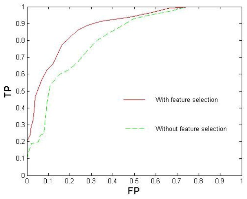
Comparison of ROC curves obtained by feature selection and without feature selection. The area sizes under ROC curve are 0.8838 and 0.8132 respectively.

4.4. Comparison of classification performance with different thresholds

Figure 4 shows a comparison of classification performance with 10 different connectivity matrix thresholds using 52-fold cross validation. Feature selection was included in all 10 cases. The AURs were 0.8838 (Th=0.4), 0.8338 (Th=0.425), 0.8299 (Th=0.5), 0.8184 (Th=0.375), 0.7922 (Th=0.475), 0.766 (Th=0.35), 0.7536 (Th=0.3), 0.7501 (Th=0.45), 0.7285 (Th=0.525) and 0.588 (Th=0.55) respectively. Since different network thresholds may highlight different outliers, overall classification accuracies can be different. The best classification performance was achieved when the network threshold was set as 0.4. In this case, by setting an appropriate classification threshold for the total number of outliers in (Eq. 10), an average sensitivity of 77.2% and specificity of 83.86% were achieved by 52-fold cross validation.

5. Discussion

The outlier rates of the five network properties summarized in table 4, indicate that ROIs such as the Hippocampus, Caudate, BA31(Superior Posterior Cingulate), BA23(Inferior Posterior Cingulate), represent the network nodes most affected in MTLE.

The hippocampus is part of the limbic system and plays an important role in epilepsy. Hippocampal sclerosis is the most commonly visible type of tissue damage in temporal lobe epilepsy although whether the epilepsy is caused by this hippocampal abnormality or the hippocampus is damaged by the cumulative effects of seizures remains uncertain. Decreased basal functional connectivity within epileptogenic networks associated with MTLE previously has been reported (Bettus et al., 2009) in a study using interictal fMRI data. The authors hypothesized that the pathophysiological alterations such as metabolic and hemodynamic changes associated with epilepsy may affect the neurovascular coupling thereby altering the relationship between BOLD signal and neuronal activity. Since it is well known that the hippocampus is involved in MTLE it is not unexpected that we observe high outlier rates on the network measures of Strength, Closeness, Degree and Clustering coefficient in hippocampus but this finding supports the utility of measuring these variables in resting-state fMRI data. The smaller Degree measure in patients suggests that there are fewer strong connections (greater than threshold) between the hippocampus and the other ROIs in MTLE. The smaller Strength values also indicate the functional connection of the hippocampus with the other ROIs appears to be generally weaker in MTLE patients compared with normal controls. The decrease observed in patients for the Closeness measure in the hippocampus also arises from fewer and weaker connections - and therefore increased distance. Outliers were found in the hippocampus in 12 out of 16 patients. More specifically, for those 10 patients whose hippocampus was clearly labeled as abnormal (table 1), outliers were found in 9 of the 10 patients. It should be noted that the abnormal seizure regions labeled in table 1 were detected by icEEG obtained in the ictal state while the outlier regions detected here were obtained from resting-state fMRI data collected in the interictal state.

The caudate nucleus is known to be an important part of the brain’s learning and memory system and as part of this system it needs to communicate with the hippocampus. Measurements of grey matter content using MRI and voxel based morphometry have revealed significant decreases in caudate volume in patients with refractory medial temporal lobe epilepsy (Bonilha 2004). In this work, the caudate demonstrates high outlier rates in the network measures of Strength, Closeness, Clustering coefficient and Betweenness centrality, a finding that also supports the use of these measures in MTLE. Most of the outliers in Strength and Closeness of caudate are negative outliers. However, there are almost equal numbers of outliers in both the negative and positive directions for the Clustering coefficient suggesting a high variation for this feature in the MTLE group compared with that of the healthy controls.

The third major abnormal node revealed by this network analysis is the Cingulate gyrus which also functions as an integral part of the limbic system, and is involved with emotion formation and processing, learning and memory, as well as the default mode network. The network measures of Strength, and Closeness for BA31(Superior Posterior Cingulate) and BA23(Inferior Posterior Cingulate) rank in the top 30 abnormal features. In the MTLE epilepsy patients the functional connections of BA31 and BA23 with other ROIs were stronger than those of normal healthy volunteers according to the high positive outlier rates of Strength, and Closeness. The increase of functional connectivity in Posterior Cingulate Cortex has also been reported in other studies of MTLE (Zhang et al., 2010). This increased connectivity in resting-state has been suggested to be involved in compensatory mechanisms (Bettus et al., 2009). Another possible interpretation is that the PCC is involved in initiation of spike and slow-wave discharges activity (Wang et al., 2011) and hence shows an up-regulated network in these patients.

The globus pallidus is a sub-cortical structure of the brain and is a major component of the basal ganglia system. It has been implicated functionally to play an active part in pre-filtering external stimuli and may help reduce the amount of irrelevant information the brain needs to store. In terms of epilepsy there is evidence for a role of the globus pallidus in the hippocampal epilepsy network (Sabatino 1984, Sawamura 2002). The network measures of Degree, Strength and Closeness showed high negative outlier rates suggesting weak connections between this ROI and other parts of the MTLE network.

Finally, the orbitofrontal cortex (OFC), also part of the limbic system, has previously also been found to be involved in the MTLE network (Blumenfeld 2004). Our network analysis indicated high positive outlier rates for the network measure of Clustering coefficient particularly in the left lateral OFC, which represents the high local embeddedness of the left OFC in the MTLE network.

Taken together, these findings of alterations in the network properties in the limbic system in MTLE patients suggest that such network measures may be valuable in assessing MTLE patients using resting-state fMRI data.

By selecting those features that have larger outlier rates in the patient group relative to healthy volunteers, a classification accuracy of AUR=0.8838 was achieved. These findings reveal that the medial temporal lobe/limbic system exhibits abnormal network properties at the group level in fMRI data obtained during the interictal state.

There are other literatures on the studying of interictal MTLE using fMRI. Liao (Liao et al., 2010) reported altered small world properties of the interictal MTLE network with fMRI. A number of areas in the default mode network including bilateral inferior frontal opercular gyrus, left posterior cingulated gyrus, left precunes and right precentral gyrus, were shown significant decreases in Degree in MTLE. Based on n-to-1 connectivity, some ROIs such as bilateral gyrus rectus, left superior frontal gyrus, left middle temporal gyrus, right middle orbitofrontal gyrus and right superior medial frontal gyrus were shown to have significantly increased connectivity in MTLE. Zhang (Zhang et al., 2009) applied independent component analysis (ICA) in a resting-state fMRI study of temporal lobe epilepsy. The functional connectivity of the dorsal attention network (DAN) was found to be decreased in patients. Morgan (Morgan et al., 2009) used 2dTCA to investigate the activation of functional network in left MTLE. The connectivity in the left anterior hippocampus, bilateral insular cortex and default-mode network was investigated and using the left anterior hippocampus as a seed region, the authors reported increased negative connectivity in the patients compared to control subjects across a network including thalamic, brainstem, frontal and parietal regions.

In our study, unlike the binary matrix used in (Liao et al., 2010), a weighted undirected connectivity matrix was adopted and matrix normalization was proposed. Using five local network properties, abnormal network properties were found in medial temporal lobe/limbic system including hippocampus, cingulated gyrus and lateral OFC as well as the caudate and globus pallidus based on the classification efficiency.

The nodes of the network analysis in this study were selected using predefined ROIs. Connectivity analysis is a region based method that relies heavily on the choice of the ROIs used for the analysis. Generalizing the ROI approach used here and performing network analyses on a voxel basis has recently been shown to reveal differences between patients and control subjects in Alzheimer’s disease (Buckner 2009). Such an approach can reveal local topology of hubs revealing both ‘connector hubs’ (hub regions that are highly connected within one module) and ‘provincial hubs’ (hub regions that link different modules) (Sporns, 2007; Hagmann, 2008) in epilepsy networks. Work is underway in our lab (Shen 2010) to develop cortical parcellation approaches based on graph theory that can use resting-state data to define functional subunits (nodes) for this type of analysis thereby decreasing the need for reliance on anatomically or atlas defined ROIs.

6. Conclusions and future work

The findings presented here indicate that network properties measured from resting-state fMRI data collected in the interictal state may reveal abnormal nodes involved in the epileptogenic network. Network theory provides measures such as Degree, Strength, Closeness, Clustering coefficient and Betweenness centrality, that appear to serve as efficient features that can distinguish healthy volunteers from medial temporal lobe epilepsy patients, even when these measures are based on data collected in the interictal state. They can extract meaningful local information about network abnormalities associated with epilepsy and identify specific nodes with abnormal connections. High outlier rates for some of the network metrics were found in the limbic system with the primary regions including the hippocampus, cingulated gyrus and lateral OFC together with caudate and globus pallidus providing the most discerning information. These findings support the notion that network analysis can reveal altered patterns of connectivity changes that are consistent across patients in a clinical category.

In this work we have introduced a functional connectivity matrix normalization method and a feature selection strategy designed to improve the classification performance of these network properties. Based on the classification criteria, an average sensitivity of 77.2% and specificity of 83.86% was achieved using 52-fold cross validation.

Further investigations on methods to improve the classification accuracy, are underway using other measurements such as coherence and partial correlation/coherence as the input to the connectivity matrix.

References

- Arora J, Pugh K, Westerveld M, Spencer S, Spencer DD, Constable RT. Language lateralization in epilepsy patients: fMRI validated with the Wada procedure. Epilepsia. 2009;50:2225–41. doi: 10.1111/j.1528-1167.2009.02136.x. [DOI] [PubMed] [Google Scholar]
- Basset DS, Bullmore E. Small-world brain networks. Neuroscientist. 2006;12:512–23. doi: 10.1177/1073858406293182. [DOI] [PubMed] [Google Scholar]
- Bertashius KM. Propagation of human complex-partial seizures: a correlation analysis. Electroencephalography and Clinical Neurophysiology. 1991;78:333–40. doi: 10.1016/0013-4694(91)90095-l. [DOI] [PubMed] [Google Scholar]
- Bettus G, Guedj E, Joyeux F, Confort-Gouny S, Soulier E, et al. Decreased basal fMRI functional connectivity in epileptogenic networks and contralateral compensatory mechanisms. Human Brain Mapping. 2009;30:1580–91. doi: 10.1002/hbm.20625. [DOI] [PMC free article] [PubMed] [Google Scholar]
- Biswal B, Yetkin FZ, Haughton VM, Hyde JS. Functional connectivity in the motor cortex of resting human brain using echo-planar mri. Magnetic Resonance in Medicine. 1995;34:537–41. doi: 10.1002/mrm.1910340409. [DOI] [PubMed] [Google Scholar]
- Bonilha L, Rorden C, Castellano G, Pereira P, Rio PA, Cendes F, Li LM. Voxel-based morphometry reveals gray matter network atrophy in refractory medial temporal lobe epilepsy. Arch Neurol. 2004;61:1379–84. doi: 10.1001/archneur.61.9.1379. [DOI] [PubMed] [Google Scholar]
- Buckner RL, Sepulcre J, Talukdar T, Krienen FM, Liu H, Hedden T, Andrews-Hanna JR, Sperling RA, Johnson KA. Cortical hubs revealed by intrinsic functional connectivity: mapping, assessment of stability, and relation to Alzheimer’s disease. The Journal of Neuroscience. 2009;29:1860–73. doi: 10.1523/JNEUROSCI.5062-08.2009. [DOI] [PMC free article] [PubMed] [Google Scholar]
- Blumenfeld H, Rivera M, McNally KA, Davis K, Spencer DD, Spencer SS. Ictal neocortical slowing in temporal lobe epilepsy. Neurology. 2004;63:1015–21. doi: 10.1212/01.wnl.0000141086.91077.cd. [DOI] [PubMed] [Google Scholar]
- Dellen EV, Douw L, Baayen JC, Heimans JJ, Ponten SC, Vandertop WP, Velis DN, Stam CJ, Reijneveld JC. Long-term effects of temporal lobe epilepsy on local neural networks: a graph theoretical analysis of corticography recordings. PLoS ONE. 2009;4(11):e8081. doi: 10.1371/journal.pone.0008081. [DOI] [PMC free article] [PubMed] [Google Scholar]
- Friston KJ, Williams S, Howard R, Frackowiak RS, Turner R. Movement-related effects in fMRI time-series. Magn Reson Med. 1996;35:346–55. doi: 10.1002/mrm.1910350312. [DOI] [PubMed] [Google Scholar]
- Grootoonk S, Hutton C, Ashburner J, Howseman AM, Josephs O, Rees G, Friston KJ, Turner R. Characterization and correction of interpolation effects in the realignment of fMRI time series. NeuroImage. 2000;11:49–57. doi: 10.1006/nimg.1999.0515. [DOI] [PubMed] [Google Scholar]
- Hagmann P, Cammoun L, Gigandet X, Meuli R, Honey CJ, Wedeen VJ, Sporns O. Mapping the structure core of human cerebal cortex. PLOS Biology. 2008;6(7):e159. doi: 10.1371/journal.pbio.0060159. [DOI] [PMC free article] [PubMed] [Google Scholar]
- Hampson M, Peterson BS, Skudlarski P, Gatenby JC, Gore JC. Detection of functional connectivity using temporal correlations in MR images. Human Brain Mapping. 2002;15:247–62. doi: 10.1002/hbm.10022. [DOI] [PMC free article] [PubMed] [Google Scholar]
- Hampson M, Driesen N, Skudlarski P, Gore JC, Constable RT. Brain connectivity related to working memory performance. J Neuroscience. 2006a;26(51):13338–43. doi: 10.1523/JNEUROSCI.3408-06.2006. [DOI] [PMC free article] [PubMed] [Google Scholar]
- Hampson M, Tokoglu F, Sun Z, Schafer RJ, Skudlarski P, Gore JC, Constable RT. Connectivity-Behavior analysis reveals that functional connectivity between left BA39 and Broca’s area varies with reading abiliy. Neuroimage. 2006b;31(2):513–519. doi: 10.1016/j.neuroimage.2005.12.040. [DOI] [PubMed] [Google Scholar]
- Hanley J, McNeil B. A method of comparing the areas under receiver operating characteristic curves derived from the same cases. Radiology. 1983;148:839–43. doi: 10.1148/radiology.148.3.6878708. [DOI] [PubMed] [Google Scholar]
- Horstmann MT, Bialonski S, Noennig N, Mai H, Prusseit J, Wellmer J, Hinrichs H, Lehnertz K. State dependent properties of epileptic brain networks: Comparative graph–theoretical analyses of simultaneously recorded EEG and MEG. Clinical Neurophysiology. 2010;121:172–85. doi: 10.1016/j.clinph.2009.10.013. [DOI] [PubMed] [Google Scholar]
- Kamada T, Kawai S. An algorithm for drawing general undirected graphs. Information Processing Letter. 1989;31:7–15. [Google Scholar]
- Kramer MA, Kolaczyk ED, Kirsch HE. Emergent network topology at seizure onset in humans. Epilepsy Research. 2008;79:173–86. doi: 10.1016/j.eplepsyres.2008.02.002. [DOI] [PubMed] [Google Scholar]
- Liao W, Zhang Z, Pan Z, Mantini D, Ding J, et al. Altered Functional Connectivity and Small-World in Mesial Temporal Lobe Epilepsy. PLoS ONE. 2010;5(1):e8525. doi: 10.1371/journal.pone.0008525. [DOI] [PMC free article] [PubMed] [Google Scholar]
- Lowe MJ, Mock BJ, Sorenson JA. Functional connectivity in single and multislice echoplanar imaging using resting-state fluctuations. NeuroImage. 1998;7:119–32. doi: 10.1006/nimg.1997.0315. [DOI] [PubMed] [Google Scholar]
- Martin JK, Hirschberg DS. Tech Report. Department of Information and Computer Science; UC Irvine: 1996. Small samples statistics for classification error rates I: Error rate measurement. [Google Scholar]
- Metz C. ROC methodology in radiological imaging. Investigate Radiology. 1986;21:720–33. doi: 10.1097/00004424-198609000-00009. [DOI] [PubMed] [Google Scholar]
- Morgan VL, Gore JC, Abou-Khalil B. Functional epileptic network in left mesial temporal lobe epilepsy detected using resting fMRI. Epilepsy Research. 2010;88:168–78. doi: 10.1016/j.eplepsyres.2009.10.018. [DOI] [PMC free article] [PubMed] [Google Scholar]
- Mullen KM, Vohr BR, Katz KH, Schneider KC, Lacadie C, Hampson M, Makuch RW, Reiss AR, Constable RT, Ment LR. Preterm birth results in alteration in neural connectivity at age 16 years. NeuroImage. 2010 doi: 10.1016/j.neuroimage.2010.11.019. [DOI] [PMC free article] [PubMed] [Google Scholar]
- Nooy WD, Mrvar A, Batagelj V. Exploratory Social Network Analysis with Pajek. Cambridge University Press; 2005. [Google Scholar]
- Onnela JP, Saramaki J, Kertesz J, Kaski K. Intensity and coherence of motifs in weighted complex networks. Phys Rev. 2005;E71:065103. doi: 10.1103/PhysRevE.71.065103. [DOI] [PubMed] [Google Scholar]
- Ponten SC, Bartolomei F, Stam CJ. Small-world networks and epilepsy: graph theoretical analysis of intracerebrally recorded mesial temporal lobe seizures. Clinical Neurophysiology. 2007;118:918–27. doi: 10.1016/j.clinph.2006.12.002. [DOI] [PubMed] [Google Scholar]
- Reijneveld JC, Ponten SC, Berendse HW, Stam CJ. The application of graph theoretical analysis to complex networks in the brain. Clinical Neurophysiology. 2007;118:2317–31. doi: 10.1016/j.clinph.2007.08.010. [DOI] [PubMed] [Google Scholar]
- Sabatino M, La Grutta V, Gravante G, La Grutta G. Interrelations between globus pallidus and hippocampal epilepsy in the cat. Archives Internationales de Physiologie et de Biochimie. 1984;92:291–6. doi: 10.3109/13813458409071169. [DOI] [PubMed] [Google Scholar]
- Shen X, Papademetris X, Constable RT. Graph-Theory Based Parcellation of Functional Subunits in the Brain from Resting-State fMRI Data. NeuroImage. 2010;50(3):1027–1035. doi: 10.1016/j.neuroimage.2009.12.119. [DOI] [PMC free article] [PubMed] [Google Scholar]
- So NK. Epilepsy surgery. Raven Press; 1991. Depth electrode studies in mesial temporal epilepsy. [Google Scholar]
- Spencer SS, Marks D, Katz A, Kim J, Spencer DD. Anatomic correlates of interhippocampal seizure propagation time. Epilepsia. 1992;33:862–73. doi: 10.1111/j.1528-1157.1992.tb02194.x. [DOI] [PubMed] [Google Scholar]
- Spencer SS, Spencer DD. Entorhinal-hippocampal interactions in medial temporal lobe epilepsy. Epilepsia. 1994;35:721–7. doi: 10.1111/j.1528-1157.1994.tb02502.x. [DOI] [PubMed] [Google Scholar]
- Spencer SS. Neural networks in human epilepsy: evidence of and implications for treatment. Epilepsia. 2002;43:219–27. doi: 10.1046/j.1528-1157.2002.26901.x. [DOI] [PubMed] [Google Scholar]
- Sporns O, Chialvo DR, Kaiser M, Hilgetag CC. Organization, development and function of complex brain networks. Trends in Cognitive Sciences. 2004;8:418–25. doi: 10.1016/j.tics.2004.07.008. [DOI] [PubMed] [Google Scholar]
- Sporns O, Honey CJ, Kotter R. Identification and classification of hubs in brain networks. PLoS ONE. 2007;2(10):e1049. doi: 10.1371/journal.pone.0001049. [DOI] [PMC free article] [PubMed] [Google Scholar]
- Spoms O, Rubinov M, Kotter R. Brain Connectivity Toolbox. http://sites.google.com/a/brain-connectivity-toolbox.net/bct/Home.
- Stam CJ, Jones BF, Nolte G, Breakspear M, Scheltens P. Small-World Networks and Functional Connectivity in Alzheimer’s Disease. Cerebral Cortex. 2007;17:92–9. doi: 10.1093/cercor/bhj127. [DOI] [PubMed] [Google Scholar]
- Sawamura A, Hashizume K, Tanaka T. Electrophysiological, behavioral and metabolic features of globus pallidus seizures induced by a microinjection of kainic acid in rats. Brain Research. 2002;935:1–8. doi: 10.1016/s0006-8993(02)02231-x. [DOI] [PubMed] [Google Scholar]
- Wang Z, Lu G, Zhang Z, Zhong Y, Jiao Q, Zhang Z, Tan Q, Tian L, Chen G, Liao W, Li K, Liu Y. Brain Res. 2011;1374:134–41. doi: 10.1016/j.brainres.2010.12.034. [DOI] [PubMed] [Google Scholar]
- Wasserman S, Faust K. SocialNetwork Analysis: Methods and Application. Cambridge University Press; 1994. [Google Scholar]
- Wennberg R, Arruda F, Quesney LF, Olivier A. Preeminence of extrahippocampal structures in the generation of mesial temporal seizures: evidence from human depth electrode recordings. Epilepsia. 2002;43:716–26. doi: 10.1046/j.1528-1157.2002.31101.x. [DOI] [PubMed] [Google Scholar]
- Zhang Z, Lu G, Zhong Y, Tan Q, Yang Z, Liao W, Chen Z, Shi J, Liu Y. Impaired attention network in temporal lobe epilepsy: A resting FMRI study. Neuroscience Letters. 2009;458:97–101. doi: 10.1016/j.neulet.2009.04.040. [DOI] [PubMed] [Google Scholar]
- Zhang Z, Lu G, Zhong Y, Tan Q, Liao W, Wang Z, Wang Z, Li K, Chen H, Liu Y. Altered spontaneous neuronal activity of the default-mode network in mesial temporal lobe epilepsy. Brain Res. 2010;1323:152–60. doi: 10.1016/j.brainres.2010.01.042. [DOI] [PubMed] [Google Scholar]