Estimation of Local Orientations in Fibrous Structures With Applications to the Purkinje System

Abstract

The extraction of the cardiac Purkinje system (PS) from intensity images is a critical step toward the development of realistic structural models of the heart. Such models are important for uncovering the mechanisms of cardiac disease and improving its treatment and prevention. Unfortunately, the manual extraction of the PS is a challenging and error-prone task due to the presence of image noise and numerous fiber junctions. To deal with these challenges, we propose a framework that estimates local fiber orientations with high accuracy and reconstructs the fibers via tracking. Our key contribution is the development of a descriptor for estimating the orientation distribution function (ODF), a spherical function encoding the local geometry of the fibers at a point of interest. The fiber/branch orientations are identified as the modes of the ODFs via spherical clustering and guide the extraction of the fiber centerlines. Experiments on synthetic data evaluate the sensitivity of our approach to image noise, width of the fiber, and choice of the mode detection strategy, and show its superior performance compared to those of the existing descriptors. Experiments on the free-running PS in an MR image also demonstrate the accuracy of our method in reconstructing such sparse fibrous structures.

I. Introduction

The development of robust image processing techniques to quantitatively characterize sparse fibrous structures is an important yet challenging problem in medical image analysis. This type of quantification provides significant insights into several biological mechanisms and can ultimately improve current diagnostic and therapeutic approaches. For instance, the extraction of coronary arteries in angiogram or retinal blood vessels in ophthalmoscope data can improve current diagnostic tools for identifying stenoses and aneurysms, or performing a timely detection of proliferative diabetic retinopathy, respectively. Similarly, the extraction of the Purkinje system (PS) can improve electrophysiological models of the heart and benefit advanced modeling studies of cardiac dysfunction. Specifically, the PS comprises specialized fibers responsible for the propagation of the electrical impulse initiating myofiber contraction and is implicated in the initiation and sustenance of arrhythmias and ventricular fibrillation [1], [2]. Recent advances in ex vivo MRI offer sufficient image resolution to identify the free-running Purkinje fibers activating endocardial structures. However, their extraction is challenging due to the presence of image noise and numerous fiber junctions. Indeed, the only existing approach for reconstructing the PS requires significant manual intervention, which is time consuming and error prone [3].

A. Overview and Paper Contributions

In this paper, we address these issues by introducing an orientation descriptor to study different fiber geometries and extract the fiber centerlines. We model the local geometry of the fibers with an orientation distribution function (ODF), a spherical function estimated as the combination of three different profiles computed by using a nonlinear filter. The modes of the ODFs, which correspond to the local fiber orientations, are then identified via spherical clustering. Finally, for centerline extraction, the resulting modes (if any) are followed to successively find points on the fiber of interest. The stages of this framework are shown in Fig. 1(a) and our contributions are the following.

Fig. 1.

(a) Important stages of the proposed framework. (b) Processed MR slice with manually delineated fibers (red) as well as PMJs and PPJs (green).

1) Estimation of ODFs

Our descriptor estimates the probability of having an oriented structure by using nonparametric statistics and employs a nonlinear filter with an oriented spatial support to encapsulate the fibers around a point of interest. The filter is used for measuring three types of statistics generating the ODF: the intensity coherence along a candidate oriented segment, the difference in appearance between the segment and the background, and the medialness of the segment. This yields a fine representation of the local fiber geometry.

2) Identification of Local Orientations

Identification of the local fiber orientations is performed by detecting the modes of the ODF via a reformulation of the mean shift algorithm for directional data. Since the algorithm finds both the number and the locations of the modes, it has the advantage of automatically identifying the different types of fiber geometries.

3) Extraction of the Purkinje Fibers

Including the PS in conduction simulations would be paramount in the study of cardiac arrhythmias. High-resolution MRI techniques only show the free-running Purkinje fibers in the cavities [3], but local geometries such as Purkinje–myocardium junctions (PMJs) and Purkinje–Purkinje junctions (PPJs) [see Fig. 1(b)] can be identified by visual inspection. Since the ODF provides an estimate of the local orientation that is sufficiently accurate to extract the fiber centerlines as pathlines, we reconstruct the PS by using a tracking algorithm, which estimates the ODF at a starting point, e.g., a PMJ, on the fiber of interest and identifies its modes as the directions to be followed. By considering the local smoothness of the resulting point trajectory, the algorithm repeats the estimation and mode detection steps at the newly identified locations until a termination criterion is met. To the authors’ knowledge, this is the first processing study that reconstructs the free-running Purkinje fibers from an MR image.

B. Related Work

The analysis of fibrous structures is a well-studied problem in pattern recognition, which finds a wide range of applications in medical image analysis. A fibrous structure often has a spatially coherent and oriented appearance pattern, which can be detected via different feature-based or model-based descriptors. Some methods [4]–[8] estimate the local orientation from the spectral decomposition of a multiscale version of the image Hessian matrix or the structure tensor, which are formed from the second-order partial derivatives of the image. Other methods measure the image gradient flux, i.e., the amount of image gradient flowing in or out of a local spherical region. Such methods have been successfully applied to centerline extraction [9] and segmentation [10]–[12] of blood vessels. However, the aforementioned descriptors are not designed to find multiple local orientations and their multiscale implementations require special attention when analyzing segments with high curvature. Thus, these methods are often used for computing a scalar measure of tubularness. This quantifies how likely it is that each voxel belongs to a tubular structure and helps the segmentation.

The goal of identifying complex fiber geometries has motivated the development of algorithms inspired by the concept of steerable filters [13]–[16]. These works aim to identify regions where multiple lines or edges intersect by applying operators that are tunable for a particular orientation. Selected methods include invertible apertured orientation filters [17], the concept of orientation space [18] computed via Gabor filters, the concept of cores [19] measuring the intensity-based medial strength, the difference of oriented appearance means [20], multiscale lineness filters [21], and polar neighborhood intensity profiles [22]. Nonetheless, they still primarily aim to improve detection and segmentation performances rather than estimating fiber orientations as accurately as possible. Alternatively, one can extend the classical descriptors to multiple orientations. For instance, a generalized tensor formulation is used in [23] to analyze multiple orientations. However, despite its success in estimating the orientations in image patches, the method does not provide a quantitative voxel-level solution to differentiate between neighboring voxels in the same patch, which limits its applicability to fiber extraction or segmentation. In addition to accurately estimate local orientations, it is crucial to identify the different types of fiber geometries if one aims to delineate the fiber centerlines via tracking. Early works [19], [24], [25] proceed by sequentially traversing coherent appearance patterns or medial points and can deal with restricted complexities, e.g., only bifurcations. Recent tracking schemes based on minimal path detection [26]–[29], particle filters [30], and multiple hypothesis analysis [31] have the same limitation.

Although this paper focuses on the analysis of sparse fibrous structures in 3-D intensity images, it is worth mentioning the concept of ODFs in high angular resolution diffusion imaging (HARDI). HARDI produces in vivo images of biological tissues by quantifying the anisotropy of water diffusion. By acquiring diffusion measurements in several gradient directions, one can estimate the ODF, a nonparametric representation of the amount of apparent diffusion in different directions [32], from the corresponding MRI signals. Due to the relationship between the signals and the tissue microstructure, the modes of the ODF are aligned with the physical orientations. The state-of-the-art methods in HARDI thereby employ such functions—see [33], [34] and references therein—which motivated us toward building a similar representation for intensity data. Nonetheless, due to the absence of a rigorous relationship between the (intensity) signal and the fibers, we solve the problem of estimating ODFs by using an orientation descriptor.

II. Local Orientation Analysis

Consider an image of a fibrous structure with a coherent intensity pattern, as illustrated in Fig. 2(a). Let x ∈ ℝ³ be a point in the image at which we want to determine the presence of an oriented structure and its orientation. Our ODF estimator takes a neighborhood around x and investigates, using nonparametric statistics, the presence of cylindrical tube(s) of length l, radius r, and oriented along s ∈ S², where S² is the unit sphere. In a probabilistic setting, one can model s, l, and r as discrete random variables¹ taking values on the sets , , and , respectively.

Fig. 2.

(a) Identifying the fiber geometry at x via oriented cylinders (a few candidate tubes in blue, optimal ones in red). (b) Support of the pivoting filter.

Assuming that l and r are independent, the ODF at x can be defined as the probability mass function (pmf)

$$p(\mathit{s};\mathit{x})=\sum _{l\in \mathcal{L}}\sum _{r\in \mathcal{R}}p(\mathit{s}\mid l,r;\mathit{x})\underset{p(l;\mathit{x})p(r;\mathit{x})}{\underbrace{p(l,r;\mathit{x})}}.$$ (1)

Here, p(s|l, r; x) is the conditional ODF given the shape parameters l and r of the tubes and p(l, r; x) is the pmf that encodes the prior information on these parameters. Notice that if l and r are assumed to be uniform, then the estimation of p(s|l, r; x) becomes the only step toward building the ODF.

A. Estimation of the Conditional ODF

In order to estimate the conditional ODF p(s|l, r; x), we propose to use a 3-D pivoting filter inspired by the 2-D filter in [35]. As depicted in Fig. 2(b), our filter has a fixed point x and a moving point f located at a distance l_F from x. Having sampled the unit sphere at N vectors {s_n} = , the segment $\overline{\mathit{xf}}$ aligns with the orientation of interest s ∈ such that f = x + l_F s. The points ${\{{\mathit{f}}_k\}}_{k=1}^{2K}$ are placed on a circle of radius r_F, centered at f such that $\overline{\mathit{xf}}\perp {\overline{\mathit{ff}}}_k$. Their role is to tightly encapsulate the candidate fiber rooted at x and oriented along s. The vectors ${\overrightarrow{\mathit{xf}}}_k$ and ${\overrightarrow{\mathit{xf}}}_{k+1}$ are separated by an angular step α = 20° and (f_k, f_{k + K}) form an antipodal pair. One can alternatively place {f_k } around x to encapsulate the fiber, but the current shape of the support is in accordance with our model, i.e., it resembles a cylinder oriented along s with length l_F and radius r_F.

Notice now that in the presence of a fibrous structure, the intensity values along the structure are expected to be coherent. In addition, the absolute intensity variation along the structure should be less than the absolute intensity variation orthogonal to the structure. Moreover, the normals to the lateral surface of the fiber should align with the image gradients at the surface. In the following discussion, we use these three principles to estimate p(s|l, r; x) assuming that the filter is constructed at x and oriented along s ∈ with l_F = l ∈ and r_F = r ∈ .

1) Appearance Profile via Intensity Coherence

Since the intensity values along a fiber segment (at x) are expected to be coherent, this profile is designed to measure this coherence by considering the voxels along $\overline{\mathit{xf}}$. Let us first denote the image domain by ࣒ ⊂ ℝ³ and the intensity value at p ∈ ࣒ by I(p)².

The intensity coherence along $\mathit{s}\sim \overrightarrow{\mathit{xf}}$ is computed as

$$A(\mathit{s}\mid l;\mathit{x})=\frac{1}{l}{\int }_0^1{\mid I(\mathit{x}+\lambda l\mathit{s})-I(\mathit{x})\mid }^2\text{d}\lambda$$ (2)

which is minimized when s aligns with the orientation of a fiber segment rooted at x [22]. The appearance profile is subsequently computed as p_A (s|l, r; x) ∞ exp(−βA(s|l; x)), ∀ r ∈ , where β > 0 is a user-specified parameter. Thus, p_A (s|l, r; x) is high when s aligns with the fiber orientation.

To demonstrate the use of the appearance profile, we use the synthetic bifurcating fiber shown in Fig. 3(a) to generate a 3-D binary image whose intensities are corrupted at varying levels of noise. Fig. 3(b) shows one image slice with eight manually selected points of analysis. Fig. 3(c) shows the profile p_A (s; x) (marginalized over uniform l and r with β = 5) at these eight points. We observe that the appearance profile provides a coarse estimate of the fiber orientation despite its sensitivity to noise. In particular, at points {1, 3, 4, 5}, p_A gives accurate yet coarse estimates of the fiber orientations, whereas at points {2, 6, 7, 8} the profiles do not have the anticipated modal shape due to noise and points being placed at boundaries or in nonfibrous regions. The profile also offers an efficient way of measuring the coherence without considering all the voxels in the tubes, but this causes the loss of discrimination among their radii. Furthermore, although (2) can be considered as the “discretized” version of the cost function minimized by the structure tensor [8], [36], the appearance profile is capable of modeling antipodally asymmetric geometries by construction.

Fig. 3.

(a) Top view of the 3-D synthetic fiber (centerline in red and low-intensity regions in blue). (b) An image slice where 1) specific regions (divided by blue lines) are corrupted at different levels of noise and 2) eight points (in red) are manually selected for analysis. (c) Appearance profiles p_A (for N = 642) whose values are color coded (blue—low, red—high) at these eight points.

2) Directional Profile via Nonlinear Filter Response

This profile is designed to measure if the absolute intensity variation along a fiber segment $\overline{\mathit{xf}}$ is less than the minimum absolute intensity variation orthogonal to that segment. In order to fully encapsulate a fiber segment of radius r, the points {f_k} are repositioned at a distance r_F = r + 1 from f. The nonlinear response of the filter at x along an orientation s is computed for each pair of antipodal points {f_j }, j ∈ {k, k + K}, as

$$D_k(\mathit{s}\mid l,r;\mathit{x})=\{\begin{array}{ll}1,\hfill & \text{if}\mid I(\mathit{f})-I(\mathit{x})\mid \le \underset{j}{min}\mid I(\mathit{f})-I({\mathit{f}}_j)\mid \hfill \\ 0,\hfill & \text{otherwise}.\hfill \end{array}$$ (3)

This response can be considered as a partial filter response for a fixed k. The cumulative filter response is computed by summing (3) over all pairs of antipodes as $D(\mathit{s}\mid l,r;\mathit{x})=1/K{\sum }_{k=1}^K{D}_k(\mathit{s}\mid l,r;x)$. This response attains its peak when s aligns with the true orientation and remains high even if there are a few erroneous partial responses due to noise. The directional profile is then defined as p_D (s|l, r; x) ∞ D(s|l, r; x).

It is worth noting that an alternative definition for the filter response would be to take the minimum absolute intensity variation from all the pairs of antipodes and set D(s|l, r; x) = 1 if it is larger than |I(f) − I(x)|. However, this would produce a strong assignment making the response too dependent on r_F. Our definition gives a softer assignment, which brings more robustness to affine changes in illumination, while keeping the filter tuned to having a high response along the true orientation. We illustrate this property by generating a set of images where the intensity of the fiber (foreground) in Fig. 3(a) is 0 and the intensity of the background gradually decreases from 1 to 0. Fig. 4 shows eight image slices and plots the value of p_D (s|r_F; x) (marginalized over l) at the true orientation s = s^* as a function of 1) the absolute intensity difference ΔI between the foreground and the background and 2) the filter radius r_F. We observe that p_D is robust to illumination changes as it does not depend on ΔI. Moreover, the profile attains its maximum value when r_F is greater than the true fiber radius r^* = 1, but it shows a nondiscriminative behavior among all r_F > r*.

Fig. 4.

Value of p_D for the true orientation s^* as a function of the absolute intensity difference ΔI and the filter radius r_F.

3) Medialness Profile via Image Gradient Flux

This profile aims to quantify how well the point f is located on the medial axis of a fiber. It uses a flux-based measure that seeks to align the inward³ normals {n_k} at points {f_k} with the image gradients at these points. The measure is computed as

$$M(\mathit{s}\mid l,r;\mathit{x})=\frac{1}{2K}\sum _{k=1}^{2K}\mid \langle {\mathit{n}}_k,\nabla I({\mathit{f}}_k)\rangle \mid$$ (4)

where n_k is the unit vector such that f = f_k + r_Fn_k, n_k = −n_{k + K}, ∇I (p) is the image gradient⁴ at p, and 〈·, ·〉 denotes the dot product. Assuming that the fiber of interest has a circular cross section, (4) would be maximized if {f_k } are placed on the boundary of the fiber. The medialness profile is then computed as p_M (s|l, r; x) ∞ M (s|l, r; x).

We illustrate the medialness profile by using the fiber shown in Fig. 3(a) to generate noisy image data with fibers of different widths. Fig. 5 shows a selected slice from each image along with the profiles p_M (s; y) marginalized over uniform l and r. We observe that p_M has an accurate modal shape for r^* ≥ 1, but it does not show two of the three modes when 2r^* = 1. Therefore, the profile yields adequate discriminative information among the search radii, but it may become unreliable for thin fibers due to inaccuracies in the computation of the image gradients.

Fig. 5.

Noisy image slices with fibers of different widths 2r^* ∈ {1, 3, 5} and the medialness profiles p_M (for N = 642) at point y.

4) Conditional ODF

Although each of the aforementioned profiles does capture the degree of tubularness around a voxel, none of them is successful on its own right. We thereby propose to combine the profiles and estimate the conditional ODF as

$$p(\mathit{s}\mid l,r;\mathit{x})\propto (p_A(\mathit{s}\mid l,r;\mathit{x})p_D(\mathit{s}\mid l,r;\mathit{x})p_M(\mathit{s}\mid l,r;\mathit{x})).$$ (5)

The rationale behind multiplying the profiles comes from the assumption that the profiles are independent given the fiber orientation. Although this assumption is quite strong, in practice we observed that (5) provides a better estimate of the local orientation than other combinations, e.g., a weighted sum, and alleviates the shortcomings of the profiles. Notably, p(s|l, r; x) is less affected by the sensitivity of p_A to noise and the nondiscriminative behavior of p_A and p_D among . Our combination strategy also yields “sharp” ODFs, i.e., ODFs having less variation around their modes, which can improve the accuracy in orientation detection. Moreover, one can incorporate (if computable) the reliabilities of the profiles into (5) for further improvements. However, notice that each profile should have modes (or high values) at directions close to the ones of the true segments so that the contributions from other profiles are not lost. Addition of the profiles would not cause such a loss, but erroneous modes may appear and corrupt the procedure unless a reliable pruning mechanism is adopted.

B. Estimation of the Shape Prior and the ODF

The term p(l, r; x) in (1) encodes the prior information on l and r. In practice, the distributions of such random variables are either assumed to be uniform or inferred from the data. In orientation estimation, we assume that l and r are uniformly distributed, but in fiber tracking, we will enforce shape regularity by replacing the prior on r with a nonuniform distribution. Once the prior is computed, the ODF p(s; x) is estimated from (1) and provides a multiscale representation due to its cumulative nature over the tubes of different shapes.

C. Detection of Local Fiber Orientations

The problem of identifying the local orientations is equivalent to finding the modes of the ODF. We solve this problem by employing a reformulation of the mean shift algorithm for directional data. The mean shift algorithm is a nonparametric kernel density estimator, which finds the number and locations of the modes of an unknown distribution via gradient ascent [37]. Given the points ${\{{\mathit{s}}_n\}}_{n=1}^N$, the true density function p(μ) is approximated as $\widehat{p}(\mathit{\mu })=Z_{\mathrm{\Phi }}{\sum }_{n=1}^N\mathrm{\Phi }({\mathit{s}}_n,\mathit{\mu };h),$, where Φ is a kernel of bandwidth h and Z_Φ is a normalization term. Radially symmetric kernels are a natural choice for Φ. The estimation can be improved by introducing adaptive bandwidths {h_n}.

We are particularly interested in clustering directional data on the unit sphere S², so we employ the von Mises–Fisher kernel Φ (s, μ; ν) = (ν/(4π sinh(ν)))exp(ν 〈s, μ〉) between two vectors s and μ with the concentration parameter ν > 0. Furthermore, since the ODF maps a vector s_n to a non-negative value ρ_n = p(s_n; ·), the weights {ρ_n} and the bandwidths {h_n ∞ 1/ν_n} can be used for obtaining a weighted estimate of the form

$$\widehat{p}(\mathit{\mu })=Z_{\mathrm{\Phi }}\sum _{n=1}^N\frac{{\rho }_n{\nu }_n}{4\pi sinh({\nu }_n)}exp({\nu }_n\langle {\mathit{s}}_n,\mathit{\mu }\rangle ).$$ (6)

Here, an adaptive bandwidth selection strategy is adopted by computing ν_n as the inverse geodesic distance between s_n and its 10th nearest neighbor. The modes of the density estimate are then located via iterative evaluations of a mapping q: S² ↦ S². Starting at an arbitrarily chosen candidate mode μ₁ ∈ , each mode is updated as μ_{j + 1} = q (μ_j) so that ∇ _μj p̂(μ_j) → 0 as j → ∞. In particular, at the jth iteration, given μ_j together with the sets {ρ_n} and {ν_n} associated with {s_n}, each mode is updated as μ_{j + 1} = μ̃_{j + 1}/||μ̃_{j + 1}||, where

$${\stackrel{\sim }{\mathit{\mu }}}_{j+1}=\sum _{n=1}^N\frac{{\rho }_n{\nu }_n^2}{sinh({\nu }_n)}exp({\nu }_n\langle {\mathit{s}}_n,{\mathit{\mu }}_j\rangle ){\mathit{s}}_n.$$ (7)

This update rule represents a Riemannian gradient ascent on S² [38]. Hence, the algorithm finds the number C and locations of the fixed points (modes) ${\{{\mathit{\mu }}^{(c)}\}}_{c=1}^C$, which are identified as the orientations of the branches rooted at the point of analysis.

D. Implementation Details

The proposed method for estimating and analyzing the ODFs is summarized in Algorithm 1. We sample the unit sphere at N = 642 predefined vectors ${\{{\mathit{s}}_n\}}_{n=1}^N=\mathcal{S}$ obtained by using a threefold tessellation of an icosahedron. Unless otherwise stated, l and r are assumed to be uniformly distributed on = {3, 4, 5} and = {0.5, 1, …, 4}, respectively, and β = 5 in the computation of p_A. For a visual demonstration, we generate a synthetic fibrous region and manually place 14 points of interest [see Fig. 6(a)] at which the ODFs and their modes are estimated [see Fig. 6(b)]. It is observed that neither the presence of adjacent structures nor varying widths of the fibers severely affect the quality of the ODFs and the detection of their modes.

Algorithm 1.

ODF estimation and identification of local orientations

1) Place the filter at the point of analysis x.

2) Consider the uniform priors p(l; x) and p(r; x) over and , respectively, and define the set of orientations as = {sn}.

3) Estimate the value of p(sn; x) from (1) using (5), ∀sn ∈ .

4) Perform spherical clustering and identify the local fiber/branch orientations as the modes ${\{{\mathit{\mu }}_{{\mathit{x}}_1}^{(c)}\}}_{c=1}^C$ of the ODF.

Fig. 6.

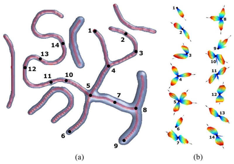
(a) Top view of the synthetic fibrous region with branching and crossing fibers of different widths and 14 points of interest at which the local ODFs are estimated. (b) 14 ODFs along with their modes (black arrows).

III. ODF-Guided Tractography

Our descriptor provides an estimate of the local orientation that is sufficiently accurate to delineate fiber centerlines even via simple tracking techniques. Algorithm 2 is an improved version of the semiautomatic method we introduced in [39], which iteratively tracks a fiber by following the local orientation estimates. The fiber is represented as a sequence of points (x₀, x₁, …, x_t) = . The first two points {x₀, x₁} are manually placed by the user. Our algorithm then estimates the ODF at x₁, detects the C mode(s) ${\{{\mathit{\mu }}_{{\mathit{x}}_1}^{(c)}\}}_{c=1}^C$ of the ODF, finds the next point(s) along the mode(s), ${\{{\mathit{x}}_2^{(c)}\}}_{c=1}^C$, and so on. Notice that when C > 1, a new branch of the initial fiber is created and tracked. To enforce the spatial regularity on the resulting trajectories, we modify the computation of the ODF by using nonuniform priors on the fiber width and smoothness. We now describe these modifications for the ith iteration.

Algorithm 2.

ODF-guided tractography in 3-D images

1) At the i-th step, place the filter at x = xi.

2) Find the radius r̃i−1 of the segment along si−1 from (8).

3) Define the first prior p(r; xi) as (r̃i−1, σ) over and the second prior p(l; xi) as uniform over .

4) ODF estimation & mode detection: Using a threefold icosahedral tessellation for discretizing the unit sphere,

a. Obtain the set i = {s: 〈s, si−1〉 > 0,s ∈ S2}. b. Estimate the value of p(sn; xi) from (10), ∀sn ∈ . c. Perform fiber/branch orientation analysis by detecting the modes ${\{{\mathit{\mu }}_{{\mathit{x}}_i}^{(c)}\}}_{c=1}^C$ of the ODF via spherical clustering.

5) Mode refinement: Having found initial estimates of the C modes, using a fourfold tessellation and for c = 1,…, C,

a. Obtain the set ${\mathcal{S}}_i^{(c)}=\{\mathit{s}:\langle \mathit{s},{\mathit{\mu }}_{{\mathit{x}}_i}^{(c)}\rangle >0.9,\mathit{s}\in S^2\}$. b. Estimate the value of p(sn; xi) from (10), $\forall {\mathit{s}}_n\in {\mathcal{S}}_i^{(c)}$. c. Refine the mode ${\mathit{\mu }}_{{\mathit{x}}_i}^{(c)}$ via spherical clustering.

6) Set ${\mathit{s}}_i^{(c)}={\mathit{\mu }}_{{\mathit{x}}_i}^{(c)}$ and find ${\mathit{x}}_{i+1}^{(c)}={\mathit{x}}_i+{\mathit{s}}_i^{(c)}$, i.e., the next point on the c-th branch, ∀c.

7) Iterate between 1–6 by setting i = i + 1 until a user-defined termination criterion is met, e.g., Σnp(sn; xi) < 0.1.

8) Obtain the tracked fiber as the sequence of points { ${\mathit{x}}_i^{(c)}$}, ∀c.

1) Prior on Fiber Width

Since the points {x_i−1, x_i } delineate the “known” portion of the fiber, they are first used for estimating its width as follows: Having positioned the filter such that x = x_i−1 and f = x_i, the radius of the segment oriented along s_i−1 ∞ x_i − x_i−1 is computed as

$${\stackrel{\sim }{r}}_{i-1}=\underset{r\in \mathcal{R}}{\text{argmax}}p({\mathit{s}}_{i-1}\mid l_{\text{F}},r;{\mathit{x}}_{i-1}).$$ (8)

This step is useful in defining a prior on the radius r at x_i, i.e., p(r; x_i), by assuming that the width does not change drastically. For simplicity, r is taken to be normally distributed at x_i, i.e., p(r; x_i) ∞ exp(−((r − r̃_i−1)²/2σ²)) with σ > 0.

2) Prior on Smoothness

To penalize sharp directional changes in the fiber trajectory, we define the smoothness profile p_S by using the von Mises–Fisher distribution over S², i.e.,

$$p_S(\mathit{s}\mid {\mathit{s}}_{i-1})\propto \frac{\nu }{4\pi sinh(\nu )}exp(\nu \langle {\mathit{s}}_{i-1},\mathit{s}\rangle )$$ (9)

where s_i−1 is the mean direction and ν > 0 is a parameter regulating the concentration around the mean direction. In our experiments, we set ν to 1. Finally, assuming that l is uniformly distributed on , the algorithm estimates the ODF p(s; x_i) as

$$p(\mathit{s};{\mathit{x}}_i)\propto \left(\sum _{l\in \mathcal{L}}\sum _{r\in \mathcal{R}}p(\mathit{s}\mid l,r;{\mathit{x}}_i)p(r;{\mathit{x}}_i)\right)p_S(\mathit{s}\mid {\mathit{s}}_{i-1})$$ (10)

and detects the modes at x_i via spherical clustering.

A. Implementation Details

The ODF-guided tracking method proceeds as outlined in Algorithm 2 and its ith iteration can be summarized as follows: the method first estimates the radius r̃_i−1 of the previously tracked segment (oriented along s_i−1) and defines the prior on r (over = {0.5, 1, …, 4}) at x_i such that r ~ (r̃_i−1, σ) with σ = 0.4. We assume that l is uniformly distributed over = {3, 4}. Next, we form the set of candidate orientations = {s: 〈s, s_i−1〉 > 0, s ∈ S²} and compute the ODF p(s; x_i). To improve the accuracy, we detect the modes of the ODF in a coarse-to-fine fashion. That is, we first compute the ODF, the modes { ${\mathit{\mu }}_{{\mathit{x}}_i}^{(c)}$}, and the number of branches C at x_i using a threefold tessellation of the hemisphere, i.e., | | = 321. We then refine the set of orientations around each mode using a fourfold tessellation of a portion of the sphere around the mode, i.e., $\mid {\mathcal{S}}_i^{(c)}\mid \approx 120$. The refined mode ${\mathit{\mu }}_{{\mathit{x}}_i}^{(c)}={\mathit{s}}_i^{(c)}$ is used for locating the next point on the cth branch as ${\mathit{x}}_{i+1}^{(c)}={\mathit{x}}_i+{\mathit{s}}_i^{(c)}$.

IV. Validation and Discussions

The performance of the proposed framework is evaluated via experiments on synthetic data as well as on the free-running Purkinje fibers in a cardiac MR image. In both cases, the evaluation is done using the quantitative measures shown in Table I. We denote the true and estimated value of a quantity u, e.g., width of a fiber segment, orientation of a branch, centerlines of a fiber, etc., by u^t and ${\mathit{u}}_Q^e$, respectively, where Q is the mode detection method, the type of orientation descriptor, or the tracking algorithm, whenever appropriate. The error in orientation estimation (in degrees) is measured by the angular discrepancy between the true and the estimated orientation at point x, denoted by $\delta (s^t,s_Q^e;\mathit{x})$, whereas the error in radius estimation is measured by the rate $\xi (r^t,r_Q^e;\mathit{x})$. The accuracy in fiber extraction is quantified by two separate measures. The first one is the spatial tracking error $\epsilon ({\mathcal{X}}^t,{\mathcal{X}}_Q^e)$ (in voxels) computed as the symmetrized Chamfer distance between the estimated trajectory ${\mathcal{X}}_Q^e=\{{\mathit{x}}_j^e\}$ and the ground truth ${\mathcal{X}}^t=\{{\mathit{x}}_i^t\}$. The second measure is the smoothness difference $\tau ({\mathcal{X}}^t,{\mathcal{X}}_Q^e)$ (in 1/voxels) computed from the symmetrized curvature (κ) difference.

TABLE I.

Performance Evaluation Measures

Angular discrepancy δ	$\delta (s^t,s_Q^e;\mathit{x})=\frac{180}{\pi }arccos(\mid \langle {\mathit{s}}^t,{\mathit{s}}_Q^e\rangle \mid )$
Width estimation error rate ξ	$\xi (r^t,r_Q^e;\mathit{x})=\mid r^t-r_Q^e\mid /r^t$
Spatial tracking error ε	$\epsilon ({\mathcal{X}}^t,{\mathcal{X}}_Q^e)=\frac{1}{2}[d_{\text{Cham}}({\mathcal{X}}^t,{\mathcal{X}}_Q^e)+d_{\text{Cham}}({\mathcal{X}}_Q^e,{\mathcal{X}}^t)]$ where $d_{\text{Cham}}({\mathcal{X}}^t,{\mathcal{X}}_Q^e)=\frac{1}{\mid {\mathcal{X}}^t\mid }{\sum }_{{\mathit{x}}_i^t\in {\mathcal{X}}^t}min\{||{\mathit{x}}_i^t-{\mathit{x}}_j^e||:{\mathit{x}}_j^e\in {\mathcal{X}}_Q^e\}$
Smoothness difference τ	$\tau ({\mathcal{X}}^t,{\mathcal{X}}_Q^e)=\frac{1}{2}[d_{\text{curv}}({\mathcal{X}}^t,{\mathcal{X}}_Q^e)+d_{\text{curv}}({\mathcal{X}}_Q^e,{\mathcal{X}}^t)]$ where $d_{\text{curv}}({\mathcal{X}}^t,{\mathcal{X}}_Q^e)=\frac{1}{\mid {\mathcal{X}}^t\mid }{\sum }_{{\mathit{x}}_i^t\in {\mathcal{X}}^t}\mid \kappa ({\mathit{x}}_i^t)-\kappa ({\widehat{\mathit{x}}}^e)\mid \text{with}{\widehat{\mathit{x}}}^e=min\{||{\mathit{x}}_i^t-{\mathit{x}}_j^e||:{\mathit{x}}_j^e\in {\mathcal{X}}_Q^e\}$

Notice that the tracking error measures are not meaningful when the local geometry is misidentified. For instance, in the case of an undetected bifurcation, i.e., a false negative (FN), only a portion of the fiber will be extracted. Thus, no matter how accurate that portion is tracked, a very large ε will be produced when one or more branches are missing. A similar situation will be encountered when a point on a nonbranching segment is identified as a junction, i.e., a false positive (FP). In that case, the effect of detecting spurious branches on ε is inevitable. These instances should be considered as errors in identifying the local geometries rather than errors in fiber tracking. Thus, we also compute the rate of misidentified geometries, i.e., false positives and false negatives. For fibers that are extracted with missing/spurious branches, we take ε (or τ) as the minimum of { $d_{\text{Cham}}({\mathcal{X}}^t,{\mathcal{X}}_Q^e),d_{\text{Cham}}({\mathcal{X}}_Q^e,{\mathcal{X}}^t)$} (or d_curv).

A. Experiments on Synthetic Data

We generate a synthetic dataset comprising 3-D images of 120 single and 120 branching fibers of radii r^t ∈ {1, 2, 3}, on which we perform local orientation analysis, estimation of fiber widths, and tractography. Each fiber is formed by fitting cubic splines through four randomly selected points in an 80 × 80 × 80 lattice. In the case of branching fibers, bifurcations are randomly selected to add further branches and the resulting centerlines are the true trajectories. To assign intensity values in a realistic manner, two intensity histograms are calculated from the MR data in Section IV-B: one from the foreground voxels (fibers) and one from the background voxels. The intensities of the foreground and background are then generated by sampling from these two histograms. The image intensities are subsequently corrupted by Rician⁵ noise to obtain data at five different SNRs. Fig. 7 shows this corruption on an image slice of the synthetic fiber in Fig. 3(a).

Fig. 7.

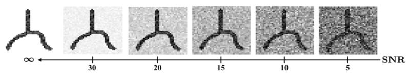
Effect of corruption with Rician noise on a synthetic image slice.

We use the aforementioned dataset to compare the ODF estimator with other well-known descriptors and our mean shift formulation with the k-means at varying noise levels. We also test the ODF-guided tracking algorithm and compare it with a minimum-cost path detection technique on real data.

1) Comparison of Mode Detection Algorithms

We focus on identifying the two branch orientations (excluding the root) at the bifurcations of 120 branching fibers. Specifically, after computing the ODF as described in Section II-D, we perform mode detection via either k-means or mean shift. Recall that the mean shift algorithm finds the number and locations of the cluster centers, which brings the advantage of avoiding the model selection problem in the k-means algorithm. It will then be natural to prefer it over k-means if their performances are comparable. For a fair analysis, however, one should first ensure that the comparison is solely performed on the geometries that are correctly identified, i.e., ODFs whose numbers of modes are correctly estimated, by the mean shift algorithm. Table II(a) presents the average rates (%) of misidentified geometries (false negatives) at varying levels of noise. The symbol “∞” for the SNR represents the noise-free case. We observe that the mean shift algorithm fails at identifying less than 2% of the geometries for SNR ≥ 15 dB, which demonstrates its accuracy in identifying bifurcations at moderately high amounts of noise.

TABLE II.

Performances of Different Mode Detection Methods at Varying Levels of Noise: (a) Average Rates (%) of Misidentified Geometries (FN) by the Mean Shift Algorithm and (b) Errors in Bifurcation Analysis in Terms of the Mean Angular Discrepancy δ (Degrees)

Error Type	SNR (dB)
	∞	30	20	15	10	5
FN	2	1	1	2	4	4
(a)

Algorithm	SNR (dB)
	∞	30	20	15	10	5
k-means	6.86	6.88	7.02	7.04	8.52	10.71
mean shift	7.51	7.87	7.90	8.23	8.53	11.52
(b)

After eliminating the false negatives, we provide the k-means algorithm with the correct number of clusters and repeat the mode detection. Table II(b) shows the mean of the angular discrepancies $\delta (s^t,s_Q^e)$ with Q ∈ {k-means, mean shift} over the remaining bifurcations at different SNRs. We observe that the mean shift algorithm achieves discrepancies of around 7.5–11.5°, which are comparable to those of the k-means algorithm. In addition, since threefold icosahedral tessellation of the sphere provides an angular resolution of around 8°, these results represent subresolution accuracies for SNR ≥ 20 dB.

2) Estimation of Local Orientations and Fiber Widths

In this experiment, we compare the proposed ODF estimator with the multiscale versions of the image Hessian matrix, the optimally oriented flux (OOF) [11], and the cores [19]. These descriptors, unlike our estimator, are tuned to find the dominant⁶ orientation at a point of interest. For a fair analysis, we thereby consider 120 single fibers and apply the descriptors to infer the local fiber geometry. Specifically, we measure the angular discrepancy $\delta (s^t,s_Q^e)$ and the width estimation error rate $\xi (r^t,r_Q^e)$ with Q ∈ {Hessian, Cores, OOF, ODF}, at 2,880 points that are evenly sampled from the centerlines of these fibers.

Estimation of Local Orientation

Here, we first apply the ODF estimator at each point of interest following Algorithm 1. For a fair comparison, we exclude the points that are misidentified, i.e., ODFs that do not show both forward and backward orientations. This corresponds to around 2% of the points when SNR≥10 dB and 12% when SNR= 5 dB. We then apply other descriptors at the remaining points.

Table III(a) presents the mean of the angular discrepancy δ over the sampled points at different SNRs. We observe that the image Hessian yields the highest discrepancies ranging from 9.33° to 14.62° with increasing levels of noise. We also see that the cores are resistant to noise with a difference of around 1.7° between its highest (8.90°) and lowest (7.16°) discrepancies. Furthermore, the errors of the OOF descriptor are smaller than those of the cores and the Hessian when SNR ≥ 10 dB, with values ranging from 6.23° to 7.30°. However, it is more sensitive to noise than the cores, with a difference of around 3.1° in discrepancy. Finally, our ODF estimator yields the lowest angular discrepancies ranging from 6.12° to 7.55° and offers a slightly improved robustness to noise.

Table III.

Performances of Different Orientation Descriptors at Varying Levels of Noise: (a) Errors in Orientation Estimation in Terms of the Mean Angular Discrepancy δ (Degrees) and (b) Mean Width Estimation Error Rates ξ (%)

Descriptor	SNR (dB)
	∞	30	20	15	10	5
Hessian	9.33	9.24	9.44	10.35	12.19	14.62
Cores	7.16	7.16	7.19	7.35	7.62	8.90
OOF	6.23	6.23	6.33	6.53	7.30	9.30
ODF	6.12	6.14	6.15	6.24	6.50	7.55
(a)

Descriptor	SNR (dB)
	∞	30	20	15	10	5
Hessian	25	25	26	25	25	22
Cores	13	13	13	14	14	17
OOF	25	25	25	25	25	22
ODF	8	8	8	8	10	12
(b)

Estimation of Fiber Width

It is worth noting that in the case of the Hessian-based and the OOF descriptors, the local orientation is identified via spectral decomposition. In the presence of a tubular structure, the eigenvector associated with the smallest eigenvalue gives the fiber orientation, whereas the other two eigenvectors can be used to measure the alignment of the (fiber) surface normals with image gradients for width estimation [11]. In the case of the cores, the measure of medialness is computed for different widths, and hence the descriptor provides such an estimate by construction. Finally, the ODF estimator infers the fiber width from (8).

Table III(b) shows the mean of the width estimation error rates ξ over the sampled points at different SNRs. We observe that while the Hessian and the OOF descriptors achieve comparable results with error rates of around 25% for SNR ≥ 10 dB, the cores yield lower rates between 13% and 17%. The ODF estimator, on the other hand, achieves the lowest errors among all descriptors, with rates ranging from 8% to 12% as the noise increases. These results justify, along with the values of the angular discrepancy in Table III(a), the reliability of the ODF estimator under noisy conditions. It is also worth noting that both the cores and our method employ similar flux-based medialness measures. The low error rates in Table III(b) indicate that such measures are particularly useful for scale estimation.

3) Extraction of Synthetic Fibers

Finally, we test the ODF-guided tracking method (following Algorithm 2 with the parameters in Section III-A) on the synthetic fibers. Table IV(a) shows the average rates (FP and FN) of misidentified geometries over 120 single and 120 branching fibers at different SNRs, whereas Table IV(b) shows the mean of the tracking errors ε and τ. We consider the misidentification of a bifurcation x^t as a false negative if x^e is not identified as a bifurcation or the position of the estimated bifurcation is not correct. We first observe that the overall FP and FN rates are less than 1% and 3% for SNR ≥ 10 dB, respectively. In particular, for SNR = 5 dB, only ten bifurcations are mislocated/missed, which affects tracking of six branching fibers out of 120. More importantly, the method yields subvoxel accuracies at all SNRs and achieves very low overall errors ε and τ of about 0.4 voxels and 0.04 voxels⁻¹ for SNR≥10 dB, respectively. Finally, Fig. 8 shows the resulting centerlines of selected fibers to visualize accurate extractions along with a few erroneous cases.

Table IV.

Performance of the ODF-Guided Tracking Method on Synthetic Fibers at Varying Levels of Noise: (a) Average Rates (%) of Misidentified Geometries (FP and FN) and (b) Extraction Performance in Terms of the Mean Spatial Tracking Error ε (Voxels) and Mean Smoothness Difference τ (1/Voxels)

Fiber Type	Error Type	SNR (dB)
		∞	30	20	15	10	5
single	FP	0.1	0.2	0.1	0.1	0.3	4.3
	FN	n/a
branching	FP	0.3	0.4	1	0.5	1.3	7.1
	FN	3	2	2	2	3	8
all	FP	0.2	0.3	0.3	0.3	0.8	5.7
	FN	3	2	2	2	3	8
(a)

Fiber Type	Error Type	SNR (dB)
		∞	30	20	15	10	5
single	ε	0.35	0.36	0.35	0.35	0.36	0.94
	τ	0.04	0.04	0.04	0.04	0.04	0.05
branching	ε	0.37	0.37	0.37	0.38	0.39	0.49
	τ	0.04	0.04	0.04	0.04	0.05	0.06
all	ε	0.36	0.36	0.36	0.37	0.38	0.72
	τ	0.04	0.04	0.04	0.04	0.04	0.06
(b)

Fig. 8.

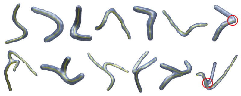
Extracted centerlines (yellow) of selected synthetic fibers at SNR = 5 dB with circular regions (red) showing algorithm failure.

B. Experiments on Real Data

To test the proposed tracking method on real data, we conduct experiments on an MR image of a healthy rabbit heart. The image is acquired [40] on an 11.7 T (500 MHz) MR system comprising a vertical magnet (bore size 123 mm; Magnex Scientific, Oxon, U.K.), a Bruker Avance console (Bruker Medical, Ettlingen, Germany), and a shielded gradient system (548 mT·m⁻¹, rise time 160 μs; Magnex Scientific, Oxon, U.K.). Quadrature driven birdcage coils with an inner diameter of 28 mm and 40 mm (Rapid Biomedical, Wurzburg, Germany) are used to transmit/receive the NMR signals. An established fast gradient echo technique is used (TE/TR = 7.5/30 ms) for high-resolution gap-free 3-D MRI, and the fixed heart is scanned with an in-plane resolution of 26.5 μm × 26.5 μm, and an out-of-plane resolution of 24.5 μm. Following the reconstruction of this unique dataset, which is publicly available [41], segmentation, denoising, and resizing steps are performed to obtain a 3-D image of size 512 × 512 × 850. Fig. 1(b) shows a slice of the processed image, where the background is almost white and the foreground has low and varying intensities. These images are comparable to the noise-free synthetic images because the intensity histograms of the foreground and the background are used to generate the data in Section IV-A.

Our algorithm is tested on the free-running Purkinje system, which is composed of 1) single fibers running from one PMJ to another and 2) branching fibers with at least one PPJ. We identified 208 Purkinje fibers with 77 PPJs, which correspond to about 80%⁷ of the free-running PS reconstructed in [3] and have varying radii (1 to 3 voxels where 1 voxel ≈ 50 μm) and intensities. For quantitative evaluation, we manually annotate the centerlines⁸ { } of the fibers and obtain the trajectories { } as explained in Algorithm 2 by using the parameters in Section III-A. We compare our method with a minimum-cost path detection algorithm implemented via fast marching [42].

Table V shows the mean and standard deviation of the spatial tracking error $\epsilon ({\mathcal{X}}^t,{\mathcal{X}}_Q^e)$ and smoothness difference $\tau ({\mathcal{X}}^t,{\mathcal{X}}_Q^e)$ with Q ∈ {minimal path, ODF-guided}, over 208 fibers, along with the rates (FP and FN) of misidentified⁹ geometries. Our algorithm yields a tracking error ε of 0.78 ± 0.37 voxels and a smoothness difference τ of 0.12 ± 0.08 voxels⁻¹, outperforming the minimal path detection method. In particular, 34 fibers are tracked with errors (ε) of less than 0.5 voxels, and 176 fibers with errors of less than 1 voxel. In addition, in the case of identifying the local geometries, the rates of false positives and false negatives are 6% and 9%, respectively. The algorithm failed at 7 PPJs by either not detecting the bifurcation or not correctly identifying the branch directions. In those cases, we observe that: 1) the thicker branch affects the ODF estimation and mode detection; 2) some of the fibers located in the vicinity of the cardiac muscle have very short (and undetected) branches; 3) some of the fibers have complex local geometries around which the structure is “sheet-like,” violating our tube model.

Table V.

Performances of Different Tracking Methods on the Free-Running Purkinje Fibers

Algorithm	Geometry ID Errors		Tracking Errors
	FP	FN	ε	τ
Minimal path	n/a	n/a	1.33 ± 1.07	0.40±0.62
ODF-guided	6	9	0.78 ± 0.37	0.12±0.08

Fig. 9(a) shows both the manually delineated and the reconstructed free-running PS. The extent of overlap demonstrates that the estimated ODFs have sufficient accuracy for extracting the PS by using a simple tracking algorithm such as ours. We also perform surface rendering of the image to show some of the resulting centerlines in Fig. 9(b) and the ODFs in Fig. 9(c).

Fig. 9.

(a) Three-dimensional illustration of the free-running PS: Ground truth fibers (red) and our reconstruction (blue) with the PMJs and PPJs (green). The centerlines are intentionally shifted relative to each other to facilitate visualization. (b) Visualization of selected Purkinje fibers and their reconstruction: 3-D rendering of selected volumes of interest (green) and the extracted centerlines (red). (c) Purkinje fiber and the ODFs estimated (for N = 2562) at six points on its centerline.

V. Concluding Remarks

We have proposed a novel descriptor to find the local fiber orientations and extract sparse fibrous structures in intensity images. Our method employs a nonlinear filter to estimate the orientation distribution function (ODF) at a point of interest. The filter is built from multiple profiles that measure the intensity coherence and medialness of the estimated structures. The estimation of the ODF is made robust by marginalizing the filter response over multiple fiber scales (length and width). The local orientations are identified as the modes of the ODF via the mean shift algorithm and guide the extraction of the fibers.

We observed via experiments on synthetic data that our descriptor provides accurate estimates of the local orientations and outperforms other well-known descriptors. First, defining the ODF as a marginal pmf prevents the restricted (fixed-scale) support of the filter from affecting the identification of local orientations. In addition, by combining different profiles, the descriptor yields sharp ODFs and is robust to moderate amounts of noise. Moreover, although our formulation contains multiple parameters, the important ones are { , }, whose values are chosen according to the fiber shape, and N, which describes a tradeoff between the computational load and accuracy. The values of the “concentration” parameters {σ, β, ν} can be selected from a large spectrum without severely affecting the performance. In principle, our method can be applied to images of other fibrous structures—see [43] for the analysis of coronary arteries in MR angiograms. However, this may require tuning the parameters { , , N}, which are application dependent.

The efficacy of the ODF-guided tracking method is demonstrated on the free-running Purkinje system, a sparse fibrous network of unique importance in cardiac electrophysiology. Compared to other stochastic tracking approaches, e.g., [30], [44], the advantage of our method is its lower computational complexity. However, its performance may deteriorate due to the accumulation of erroneous local estimates. In the case of the Purkinje fibers, this occurs around a number of bifurcations at which our tube model is violated. A promising strategy to resolve such cases would be to preclassify the geometries, inspired by the descriptors that are capable of identifying “tube-like,” “sheet-like,” or “blob-like” structures [12]. Nonetheless, the reconstructed PS is very accurate for our ultimate goal of advancing realistic modeling of cardiac function.

Biographies

Hasan E. Çetingül (S’03) received the B.S. degree in electrical and electronics engineering and the minor in business administration from Middle East Technical University, Ankara, Turkey, in 2003. He received the M.S. degree in electrical and computer engineering from Koç University, Istanbul, Turkey, in 2005. He is currently working toward the Ph.D. degree in biomedical engineering from the Johns Hopkins University, Baltimore, MD.

He was a Visiting Researcher in the Signal Processing Laboratory 5 of the Swiss Federal Institute of Technology (EPFL), Lausanne, Switzerland, on August 2004. His research interests include medical image analysis, computer vision, machine learning, and biometrics, with emphasis on segmentation, manifold clustering, and audiovisual speaker/speech recognition.

Gernot Plank received the M.S. and Ph.D. degrees in electrical engineering from the Institute of Biomedical Engineering, Technical University of Graz, Graz, Austria, in 1996 and 2000, respectively.

He is currently an Associate Professor with the Institute of Biophysics, Medical University of Graz, Graz, Austria, and Academic Fellow with the Computational Biology Group, University of Oxford, Oxford, U.K. Prior to this, he was a Postdoctoral Fellow with the Technical University of Valencia, Spain, from 2000 to 2002, the University of Calgary, Calgary, AB, Canada, in 2003, and a Marie Curie Fellow with the Johns Hopkins University, Baltimore, MD, from 2006 to 2008. His research interests include computational modeling of cardiac bioelectric activity, microscopic mapping of the cardiac electric field, and defibrillation.

Natalia A. Trayanova (A’90–SM’91) received the Ph.D. degree from the Bulgarian Academy of Sciences, Sofia, Bulgaria.

She is currently a Professor in the Department of Biomedical Engineering and the Institute for Computational Medicine at the Johns Hopkins University, Baltimore, MD, and the inaugural William R. Brody Faculty Scholar. Her research interests include understanding the normal and pathological electrophysiological and electromechanical behavior of the heart, with emphasis on the mechanisms for cardiac arrhythmogenesis and defibrillation, the role of cardiac tissue structure, and the mechanoelectric feedback in the heart.

René Vidal (M’98) received the B.S. degree in electrical engineering (highest hons.) from the Pontificia Universidad Católica de Chile, Santiago, Chile, in 1997, and the M.S. and Ph.D. degrees in electrical engineering and computer sciences from the University of California at Berkeley, Berkeley, in 2000 and 2003, respectively.

He is currently an Associate Professor in the Department of Biomedical Engineering and the Center for Imaging Science at Johns Hopkins University, Baltimore, MD. He was a Research Fellow at the National ICT Australia in 2003. He was a co-editor of the book Dynamical Vision and has coauthored numerous articles in biomedical image analysis, computer vision, machine learning, hybrid systems, and robotics.

References

- 1.Dosdall D, Taberaux P, Kim J, Walcott G, Rogers J, Killingsworth C, Huang J, Robertson P, Smith W, Ideker R. Chemical ablation of the Purkinje system causes early termination and activation rate slowing of long duration ventricular fibrillation in dogs. AJP—Heart Circulatory Physiol. 2008;295(2):H883–H889. doi: 10.1152/ajpheart.00466.2008. [DOI] [PMC free article] [PubMed] [Google Scholar]
- 2.Deo M, Boyle P, Plank G, Vigmond E. Arrhythmogenic mechanisms of the Purkinje system during electric shocks: A modeling study. Heart Rhythm. 2009;6(12):1782–1789. doi: 10.1016/j.hrthm.2009.08.023. [DOI] [PMC free article] [PubMed] [Google Scholar]
- 3.Vadakkumpadan F, Rantner L, Tice B, Boyle P, Prassl A, Vigmond E, Plank G, Trayanova N. Image-based models of cardiac structure with applications in arrhythmia and defibrillation studies. J Electrocardiol. 2009;42:157. e1–157. e10. doi: 10.1016/j.jelectrocard.2008.12.003. [DOI] [PMC free article] [PubMed] [Google Scholar]
- 4.Sato Y, Nakajima S, Shiraga N, Atsumi H, Yoshida S, Koller T, Gerig G, Kikinis R. 3D multi-scale line filter for segmentation and visualization of curvilinear structures in medical images. Med Image Anal. 1998;2(2):143–168. doi: 10.1016/s1361-8415(98)80009-1. [DOI] [PubMed] [Google Scholar]
- 5.Frangi A, Niessen W, Hoogeveen R, van Walsum T, Viergever M. Model-based quantitation of 3D magnetic resonance angiographic images. IEEE Trans Med Imag. 1999 Oct;18(10):946–956. doi: 10.1109/42.811279. [DOI] [PubMed] [Google Scholar]
- 6.Krissian K, Malandain G, Ayache N, Vaillant R, Trousset Y. Model based detection of tubular structures in 3D images. Comput Vis Image Understand. 2000;80(2):130–171. [Google Scholar]
- 7.Manniesing W, Viergever M. Vessel enhancing diffusion: A scale space representation of vessel structures. Med Image Anal. 2006;10(6):815–825. doi: 10.1016/j.media.2006.06.003. [DOI] [PubMed] [Google Scholar]
- 8.Brox T, Weickert J, Burgeth B, Mràzek P. Nonlinear structure tensors. Image Vis Comput. 2006;24(1):41–55. [Google Scholar]
- 9.Bouix S, Siddiqi K, Tannenbaum A. Flux driven automatic center-line extraction. Med Image Anal. 2005;9(3):209–221. doi: 10.1016/j.media.2004.06.026. [DOI] [PubMed] [Google Scholar]
- 10.Vasilevskiy A, Siddiqi K. Flux maximizing geometric flows. IEEE Trans Pattern Anal Mach Intell. 2002 Dec;24(12):1565–1578. [Google Scholar]
- 11.Law M, Chung A. Three dimensional curvilinear structure detection using optimally oriented flux. In: Forsyth D, Torr P, Zisserman A, editors. Computer Vision—ECCV (series LNCS 5305) Berlin/Heidelberg. Germany: Springer; 2008. pp. 368–382. [Google Scholar]
- 12.Descoteaux M, Collins L, Siddiqi K. A geometric flow for segmenting vasculature in proton-density weighted MRI. Med Image Anal. 2008;12(4):497–513. doi: 10.1016/j.media.2008.02.003. [DOI] [PubMed] [Google Scholar]
- 13.Freeman W, Adelson E. The design and use of steerable filters. IEEE Trans Pattern Anal Mach Intell. 1991 Sep;13(9):891–906. [Google Scholar]
- 14.Michaelis M, Sommer G. Junction classification by multiple orientation detection. In: Eklundh J-O, editor. Computer Vision—ECCV (series LNCS 800) Berlin/Heidelberg, Germany: Springer-Verlag; 1994. pp. 101–108. [Google Scholar]
- 15.Perona P. Steerable-scalable kernels for edge detection and junction analysis. In: Sandini G, editor. Computer Vision—ECCV (series LNCS 588) Berlin/Heidelberg, Germany: Springer-Verlag; 1992. pp. 3–18. [Google Scholar]
- 16.Simoncelli E, Farid H. Steerable wedge filters for local orientation analysis. IEEE Trans Image Process. 1996 Sep;5(12):1377–1382. doi: 10.1109/83.535851. [DOI] [PubMed] [Google Scholar]
- 17.Kalitzin S, Romeny BTH, Viergever M. Invertible apertured orientation filters in image analysis. Int J Comput Vis. 1999;31(2):145–158. [Google Scholar]
- 18.Chen J, Sato Y, Tamura S. Orientation space filtering for multiple orientation line segmentation. IEEE Trans Pattern Anal Mach Intell. 2000 May;22(5):417–429. [Google Scholar]
- 19.Fridman Y, Pizer S, Aylward S, Bullitt E. Extracting branching tubular object geometry via cores. Med Image Anal. 2004;8:169–176. doi: 10.1016/j.media.2004.06.017. [DOI] [PubMed] [Google Scholar]
- 20.Galun M, Basri R, Brandt A. Multiscale edge detection and fiber enhancement using differences of oriented means. Proc IEEE Int Conf Comput Vis. 2007:1–8. [Google Scholar]
- 21.Bennink H, van Assen H, Streekstra G, ter Wee R, Spaan J, ter Haar Romeny B. A novel 3D multi-scale lineness filter for vessel detection. In: Ayache N, Ourselin S, Maeder A, editors. Medical Image Computing and Computer-Assisted Intervention (series LNCS 4792) Berlin/Heidelberg, Germany: Springer-Verlag; 2007. pp. 436–443. [DOI] [PubMed] [Google Scholar]
- 22.Qian X, Brennan M, Dione D, Dobrucki W, Jackowski M, Breuer C, Sinusas A, Papademetris X. A non-parametric vessel detection method for complex vascular structures. Med Image Anal. 2009;13:49–61. doi: 10.1016/j.media.2008.05.005. [DOI] [PMC free article] [PubMed] [Google Scholar]
- 23.Mühlich M, Aach T. Analysis of multiple orientations. IEEE Trans Image Process. 2009 Jul;18(7):1424–1437. doi: 10.1109/TIP.2009.2019307. [DOI] [PubMed] [Google Scholar]
- 24.Flasque N, Desvignes M, Constans JM, Revenu M. Acquisition, segmentation and tracking of the cerebral vascular tree on 3D magnetic resonance angiography images. Med Image Anal. 2001;5:173–183. doi: 10.1016/s1361-8415(01)00038-x. [DOI] [PubMed] [Google Scholar]
- 25.Alyward S, Bullitt E. Initialization, noise, singularities, and scale in height ridge traversal for tubular object centerline extraction. IEEE Trans Med Imag. 2002 Feb;21(2):61–75. doi: 10.1109/42.993126. [DOI] [PubMed] [Google Scholar]
- 26.Wink O, Niessen W, Viergever M. Multiscale vessel tracking. IEEE Trans Med Imag. 2004 Jan;23(1):130–133. doi: 10.1109/tmi.2003.819920. [DOI] [PubMed] [Google Scholar]
- 27.Li H, Yezzi A. Vessels as 4-D curves: Global minimal 4-D paths to extract 3-D tubular surfaces and centerlines. IEEE Trans Med Imag. 2007 Sep;26(9):1213–1223. doi: 10.1109/tmi.2007.903696. [DOI] [PubMed] [Google Scholar]
- 28.Péchaud M, Keriven R, Peyré G. Proc IEEE Conf Comput Vis Pattern Recognit. 2009. Extraction of tubular structures over an orientation domain; pp. 336–342. [Google Scholar]
- 29.Benmansour F, Cohen L, Law M, Chung A. Tubular anisotrophy for 2D vessels segmentation. Proc IEEE Conf Comput Vis Pattern Recognit. 2009:2286–2293. [Google Scholar]
- 30.Florin C, Paragios N, Williams J. Globally optimal active contours, sequential monte carlo and on-line learning for vessel segmentation. In: Leonardis A, Bischof H, Pinz A, editors. Computer Vision - ECCV (series LNCS 3953) Berlin/Heidelberg, Germany: Springer-Verlag; 2006. pp. 476–489. [Google Scholar]
- 31.Friman O, Hindennach M, Kühnel C, Peitgen HO. Multiple hypothesis template tracking of small 3D vessel structures. Med Image Anal. 2009;14:160–171. doi: 10.1016/j.media.2009.12.003. [DOI] [PubMed] [Google Scholar]
- 32.Tuch D. Q-ball imaging. Magn Reson Med. 2004;52(6):1358–1372. doi: 10.1002/mrm.20279. [DOI] [PubMed] [Google Scholar]
- 33.Alexander D. Multiple-fibre reconstruction algorithms for diffusion MRI. Ann NYAS. 2005;1064:113–133. doi: 10.1196/annals.1340.018. [DOI] [PubMed] [Google Scholar]
- 34.Descoteaux M, Deriche R, Knoesche T, Anwander A. Deterministic and probabilistic tractography based on complex fiber orientation distributions. IEEE Trans Med Imag. 2009 Feb;28(2):269–286. doi: 10.1109/TMI.2008.2004424. [DOI] [PubMed] [Google Scholar]
- 35.Geman D, Jedynak B. An active testing model for tracking roads in satellite images. IEEE Trans Pattern Anal Mach Intell. 1996 Jan;18(1):1–14. [Google Scholar]
- 36.Bertram M, Wiegert J, Schäfer D, Aach T, Rose G. Directional view interpolation for compensation of sparse angular sampling in cone-beam CT. IEEE Trans Med Imag. 2009 Jul;28(7):1011–1022. doi: 10.1109/TMI.2008.2011550. [DOI] [PubMed] [Google Scholar]
- 37.Comaniciu D, Meer P. Mean Shift: A robust approach toward feature space analysis. IEEE Trans Pattern Anal Mach Intell. 2002 May;24(5):603–619. [Google Scholar]
- 38.Çetingül H, Vidal R. Intrinsic mean shift for clustering on Stiefel and Grassmann manifolds. Proc IEEE Conf Comput Vis Pattern Recognit. 2009:1896–1902. [Google Scholar]
- 39.Çetingül H, Plank G, Trayanova N, Vidal R. Estimation of multimodal orientation distribution functions from cardiac MRI for tracking Purkinje fibers through branchings. Proc IEEE Int Symp Biomed Imag. 2009:839–842. [Google Scholar]
- 40.Burton R, Plank G, Schneider J, Grau V, Ahammer H, Keeling S, Lee J, Smith N, Gavaghan D, Trayanova N, Kohl P. Three-dimensional models of individual cardiac histoanatomy: Tools and challenges. Ann NYAS. 2006;1080:301–319. doi: 10.1196/annals.1380.023. [DOI] [PMC free article] [PubMed] [Google Scholar]
- 41.Bishop M, Plank G, Burton R, Schneider J, Gavaghan D, Grau V, Kohl P. Development of an anatomically detailed MRI-derived rabbit ventricular model and assessment of its impact on simulations of electrophysiological function. AJP–Heart Circ Physiol. 2010;298(2):H699–H718. doi: 10.1152/ajpheart.00606.2009. [DOI] [PMC free article] [PubMed] [Google Scholar]
- 42.Sethian J. Level Set Methods and Fast Marching Methods. 2. New York: Cambridge Univ. Press; 1999. [Google Scholar]
- 43.Çetingül H, Gülsün M, Tek H. A unified minimal path tracking and topology characterization approach for vascular analysis. In: Liao H, Edwards P, Pan X, Fan Y, Yang G-Z, editors. Medical Imaging and Augmented Reality (series LNCS 6326) Berlin/Heidelberg, Germany: Springer-Verlag; 2010. pp. 11–20. [Google Scholar]
- 44.Schaap M, Smal I, Metz C, van Walsum T, Niessen W. Bayesian tracking of elongated structures in 3D images. In: Karssemeijer N, Lelieveldt B, editors. Information Processing in Medical Imaging (series LNCS 4584) Berlin/Heidelberg, Germany: Springer-Verlag; 2007. pp. 74–85. [DOI] [PubMed] [Google Scholar]