Pooling Data When Analyzing Biomarkers Subject to a Limit of Detection

Abstract

The use of biomarkers to assess exposure and investigate biomedical questions is common in epidemiology. The usefulness of biomarker research, however, is contingent upon the ability to achieve a complete understanding of the role they play within a population. In estimating distributional parameters for a particular biomarker, such as oxidative stress or antioxidant markers, scientists face two main challenges: overcoming the cost of performing a large number of assays and dealing with data subject to a limit of detection. While approaches have been suggested to deal with each of these issues individually, pooling is a strategy that can address both problems.

1. Introduction

The use of biomarkers to assess exposure and investigate biomedical questions is common in epidemiology. Implications of exploring the relationship between biomarker levels and outcome can have profound effects on the biomedical community, leading to new research as well as increased diagnostic capabilities. The usefulness of biomarker research, however, is contingent upon the ability to achieve a complete understanding of the role they play within a population. We have previously published protocols for using biomarkers of oxidative stress for discriminating between individuals with a disease and a normal population (1) as well as for test performance (2).

In estimating distributional parameters for a particular biomarker, such as oxidative stress or antioxidant markers, scientists face two main challenges: overcoming the cost of performing a large number of assays and dealing with data subject to a limit of detection. The power gained by a large sample must be weighed against the cost of performing more assays. After reproducibility and variability are established for the biomarker, financial constraints often limit further evaluation to small sets of samples. Instrument sensitivity may also be problematic when studying levels of oxidative stress in biological samples. Some members of the population may have serum levels below a detection threshold, d (3). Under these circumstances, values at or above the detection threshold which is designated (d) are measured and reported, but values below the detection threshold are unobservable, limiting the information one can utilize in his or her analysis.

While approaches have been suggested to deal with each of these issues individually, pooling is a strategy that can address both problems. In this method, two or more specimens are physically combined into a single “pooled” unit for analysis. Thus, a greater portion of the population is assayed for the same price; and, information per assay increases meaning fewer assays are needed to achieve equivalent information (4, 5, 6, 7). Additionally, pooling the specimens reduces the effective variance of the biomarker. This can ultimately decrease the proportion of observations below the detection threshold and increase the amount of information that can be derived from the data. Such results are useful when studying biomarkers that may naturally exist in small quantities, such as oxidative stress markers.

Pooling can be seen as a primary tool for case-control and cohort studies exploring discrete outcomes. Since it minimizes cost as well as the amount of information lost due to the detection threshold, the use of pooled data is preferable (in a context of a parametric estimation) to using all available individual measurements for certain values of d. This chapter is designed to explain how this method can be applied in such studies while discussing the benefits of the pooling strategy and the circumstances under which it is most useful.

2. Materials

Statistical software to perform analysis with data subject to limits of detection is available upon request at schistee@mail.nih.gov.

3. Methods

3.1. Formulas and Terminology

1. Suppose we have biologic specimens from a patient population, A, consisting of N individuals and wish to analyze any oxidative stress biomarker. The population, A = {A₁, A₂, … , A_N}, has test results X = {X₁, X₂, … ,X_N}. In the pooling strategy, samples from patient population A are randomly combined into n pooled specimens of size p, where n = N/p. The n pooled assays are considered the average of the contributing individual results, i.e.:

   $$\begin{array}{cc}\hfill X\left(p\right)=& \{X_1^{\left(p\right)},X_2^{\left(p\right)},\dots ,X_n^{\left(p\right)}\}\hfill \\ \hfill & =\phantom{\{}\left(X_{k_{11}}+\dots +X_{k_{1p}}\right),\frac{1}{p}\left(X_{k_{21}}+\dots +X_{k_{2p}}\right),\dots ,\frac{1}{p}\left(X_{k_{n1}}+\dots +X_{k_{np}}\right)\},\hfill \end{array}$$

   where {k_1i,i = 1, … ,p}, … ,{k_ni,i = 1, … ,p} are some disjoint subsequences of set {1,2,3, … ,N}.

2. Random sampling, another method of cost-effective sampling, selects a random sample of the patient population A^(r) = {A_k1,A_k2, … ,A_kn}∈ A, where n(≤N) is determined by a power calculation and {k_i,i = 1, … ,n} is a subsequence of set {1,2,3, … ,N} where assays are performed on the subset of specimens with observed results {X_k1,X_k2, … ,X_kn}.

3. In practice, serum levels of a biomarker of interest may fall below a detection threshold resulting in unavailable test results. When looking at population A’s results, instead of X, we observe Z = {Z₁,Z₂, …}, such that:

   $$Z_i=\{\begin{array}{cc}{X}_i,\hfill & \text{if}{X}_i\ge d;\hfill \\ \text{Not Available}(\mathrm{N}∕\mathrm{A}),\hfill & \text{if}{X}_i<d,\hfill \end{array}\phantom{\}}$$

   where d is the value of the detection threshold.

Likewise, in the pooling design, we observe Z^(p) = {Z₁^(p), … , Z_n^(p)}, where:

$$Z_i^{\left(p\right)}=\{\begin{array}{cc}{X}_i^{\left(p\right)},\hfill & \text{if}{X}_i^{\left(p\right)}\ge d;\hfill \\ \mathrm{N}∕\mathrm{A},\hfill & \text{if}{X}_i^{\left(p\right)}>d.\hfill \end{array}\phantom{\}}$$

3.2. Statistical Background of Pooling with Data Subject to a Detection Threshold

1. When dealing with data that is subject to a detection threshold, the pooling strategy is more or less beneficial depending on the location of d in relation to the mean, μ. In determining the effectiveness of this method, it is important to consider the following three cases:

   • 1.1
     When the detection threshold is below the mean, d < μ.
   • 1.2
     When the detection threshold is above the mean, μ < d.
   • 1.3
     When the detection threshold is far above the mean, μ << d.

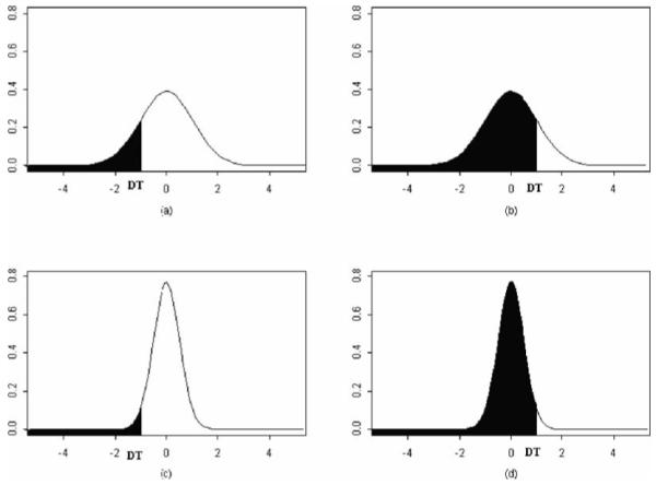
2. First, consider the case of a population, X, normally distributed around a mean of 0 that is subject to a detection threshold somewhere below the mean X ~ N(μ = 0,σ_X² = 1), μ > d. In this case, pooling takes advantage of the statistical properties of averages through physical implementation, i.e., the value of pooled specimens is the mean of the individual biomarker values. More numeric observations are available because the pooled distribution X^(p) with var(X^(p)) = σ_X²/p is more concentrated around the expectation μ = 0.

3. Next, consider the case where the detection threshold is above the mean X ~ N(μ = 0, σ_X² = 1), μ < d. In this case, pooling can be detrimental. With over half of the data below the detection threshold, more pooled samples have values below d than unpooled samples.

   Never the less, in this situation, the pooling strategy might still be more efficient than random sampling. Intuitively, the pooled observations might be more informative than the unpooled observations because each pooled observation is based on more than one test result.

4. Lastly, consider the case where the detection threshold is far above the mean d >> μ = EX. When the detection threshold is much greater than the mean biomarker value, the pooling strategy is completely inefficient because the pooled data are based upon substantially less numeric information than a random sample of unpooled data.

5. For clarity, the above cases assumed X has a normal distribution; however, the conclusions from this section are true for most commonly used distributions, including gamma.

3.3. Applications

1. Figure 31.1A plots the density function of the normally distributed biomarker X with a detection threshold at d = −1. The shaded area corresponds to values of X below d where missing values would be reported. The un-shaded area corresponds to reportable numeric values of X. In this case, since Pr{X₁ < −1} ≈ 0.16, the expected proportion of observations below d is approximately 16%. Pooling the specimens reduces the effective variance of biomarker X. The variance of the pooled samples is var(X^(p)) = σ_X²/p (4). Assuming p = 2, Pr{X₁^(p) < −1} ≈ 0.08 leaving only approximately 8% of the pooled observations that are below d as shown in Fig. 31.1C. Thus, pooling the samples cut the amount of unobservable values by half.

2. Figure 31.1B and d depict when the location of the detection threshold is above the mean of X. As shown in Fig. 31.1B, the amount of unobserved data (shaded area) is smaller in the unpooled data than in the pooled data.

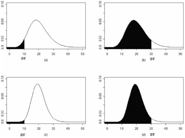
3. Figure 31.2 shows an example of pooling with gamma data (χ²₍₂₀₎ for unpooled data and χ²₍₄₀₎ for pooled data). Clearly, pooling with gamma data leads to similar conclusions as found in working with Normal distributions.

Fig. 31.1.

Normally distributed data constrained by a detection threshold (shaded area represents unobserved data).

Fig. 31.2.

Chi-square distributed data constrained by a detection threshold (shaded area represents unobserved data).

References

- 1.Schisterman E. Methods in Molecular Biology. Vol. 186. Humana Press; New Jersey: 2002. Statistical Correction of the Area Under the ROC Curve in the Presence of Random Measurement Error and Applications to Biomarkers of Oxidative Stress. [DOI] [PubMed] [Google Scholar]
- 2.Schisterman E. Methods in Molecular Biology. Vol. 196. Humana Press; New Jersey: 2002. Statistical Analysis: Receiver Operating Characteristic (ROC) Curve and Lipid Peroxidation. [DOI] [PubMed] [Google Scholar]
- 3.Helsel D. Nondetects and Data Analysis: Statistics for Censored Environ-mental Data. John Wiley & Sons, Inc.; Hoboken, New Jersey: 2005. [Google Scholar]
- 4.Faraggi D, Reiser B, Schisterman EF. ROC curve analysis for biomarkers based on pooled assessments. Statistics in Medicine. 2003;22:2515–2527. doi: 10.1002/sim.1418. [DOI] [PubMed] [Google Scholar]
- 5.Liu A, Schisterman EF. Sample size and power calculation in comparing diag-nostic accuracy of biomarkers with pooled assessments. Journal of Applied Statistics. 2004;31:41–51. [Google Scholar]
- 6.Liu A, Schisterman E. Comparison of diagnostic accuracy of biomarkers with pooled assessments. Biometrical Journal. 2003;45:631–644. [Google Scholar]
- 7.Schisterman EF, Perkins NJ, Liu A, Bondell H. Optimal cut-point and its corresponding Youden Index to discriminate individuals using pooled blood samples. Epidemiology. 2005;16:73–81. doi: 10.1097/01.ede.0000147512.81966.ba. [DOI] [PubMed] [Google Scholar]