Old and new challenges in using species diversity for assessing biodiversity

Abstract

Although the maintenance of diversity of living systems is critical for ecosystem functioning, the accelerating pace of global change is threatening its preservation. Standardized methods for biodiversity assessment and monitoring are needed. Species diversity is one of the most widely adopted metrics for assessing patterns and processes of biodiversity, at both ecological and biogeographic scales. However, those perspectives differ because of the types of data that can be feasibly collected, resulting in differences in the questions that can be addressed. Despite a theoretical consensus on diversity metrics, standardized methods for its measurement are lacking, especially at the scales needed to monitor biodiversity for conservation and management purposes. We review the conceptual framework for species diversity, examine common metrics, and explore their use for biodiversity conservation and management. Key differences in diversity measures at ecological and biogeographic scales are the completeness of species lists and the ability to include information on species abundances. We analyse the major pitfalls and problems with quantitative measurement of species diversity, look at the use of weighting measures by phylogenetic distance, discuss potential solutions and propose a research agenda to solve the major existing problems.

1. Introduction

The term ‘biodiversity’ is relatively recent with its formal introduction often pegged to the National Forum on BioDiversity, held in Washington, DC in September 1986. The published Proceedings of this forum is the first book with the term ‘biodiversity’ in its title [1]. Biodiversity has since become a central concern in social and political discussions (e.g. the Rio environmental summit meeting in 1992), matching its fundamental place in the science of ecology [2]. The increasing threat of species extinction through habitat degradation, global change and human population pressure magnified these concerns. In 2002, the United Nations declared 2010 the International Year of Biodiversity with a goal of halting by 2010 the erosion of biodiversity. Despite important efforts to prevent its loss, the biodiversity of our planet continues to decline, with no evidence of reversing this trend [3].

Fundamental to global political concerns is the potential relationship between biodiversity and ecosystem services [4,5] and the threat to those services from biodiversity loss [6,7]. The link between biodiversity and ecosystem services has been controversial, in part because we lack a consensus about the methods to assess and monitor biodiversity, especially at regional to continental scales [6–12]. Biodiversity can be quantified at many levels of biological organization—from the molecular to the ecosystem [13,14]. However, it is not practical to measure biodiversity at all levels in all places, so biodiversity assessment methods must be optimized to the specific level of organization and spatial scale of interest. For example, proxy measures (e.g. satellite imagery) of large areas can be calibrated with other data (e.g. surveys on the ground). Therein lies the problem—what proxies are best used for which measures of biodiversity (e.g. [15,16])? Species diversity is one of the most intuitive and widely adopted measures of biodiversity [17] and it is strongly positively correlated with diversity at other levels of organization, such as genetic diversity and ecosystem functioning (although mechanistic explanations are still debated [12,17]). While the measurement of species diversity has a long theoretical and empirical history within ecology [18–21], problems remain in its measurement and monitoring, especially at larger spatial extents. These larger extents are often investigated with biogeographic approaches (see §2), even when answering questions more appropriate to ecological approaches [22]. The acceleration of biodiversity loss makes urgent the development of programmes to assess and monitor biodiversity suitable for addressing large-scale ecological questions.

We examine how species diversity is used to assess and monitor biodiversity from an ecological perspective and discuss the resulting theoretical and practical advantages and limitations in using such an approach at scales that are more typically considered biogeographic. To do this we (i) define how ecological and biogeographic perspectives differ in terms of temporal and spatial scales and types and quality of data, (ii) review recent advances in analysing species diversity, (iii) examine practical issues and major pitfalls connected with the measurement of species diversity at larger spatial and temporal extents using an ecological approach, and (iv) propose a research agenda to solve these problems. In a complementary paper, Davies & Buckley [23] consider the alternative use of phylogenetic diversity for focusing at broad biogeographic scales.

2. Ecological and biogeographic perspectives

Because the preservation of biodiversity is an issue from local to global scales, we must consider the strengths and weaknesses connected with ecological and biogeographic perspectives (table 1). The differences in these perspectives primarily relate to practical considerations. The theoretical roots of ecology and biogeography are well entangled; for example, the theory of island biogeography [24] is widely considered to be fundamental in ecology [25]. Similarly, the theoretical underpinnings of both perspectives rely on evolutionary theory [25,26] and systematics [27], although currently those linkages are stronger for biogeography.

Table 1.

Comparison of ecological and biogeographic perspectives with regard to their typical spatial and temporal realms of interests, data collection, data types and data quality.

	ecology	biogeography
spatial scale	local to regional	regional to global
temporal scale	up to decades (centuries)	centuries to aeons
data collection	specific/single study	adapted/assembled studies
data types	richness and abundance	richness
data quality	high/homogeneous	variable/heterogeneous

Despite these linkages, the investigation of species diversity offers different challenges from ecological and biogeographic perspectives. In biogeography, species diversity is typically analysed as patterns of species richness across large spatial extents (regional to continental to global) or during long temporal durations (centuries to millennia to aeons). Examples include global analyses of species–area relationships in islands and continents (e.g. [28]) and latitudinal patterns of species richness (e.g. [29]). In contrast, an ecological perspective investigates species diversity at smaller spatial scales and shorter temporal scales (table 1). Examples include studies of assembly rules for community organization and structure (e.g. [30]), the relationship between species diversity and productivity (e.g. [31]), and the role of evenness and richness in structuring communities (e.g. [32]).

The two perspectives also differ in data collection, type and quality. Biogeographic investigations are largely based on datasets assembled from multiple sources, carried out over many years or decades, because measuring species presences and abundances over a large area by a single team of people is almost infeasible. At biogeographic scales, data are typically limited to measures of species richness and these can be heterogeneous and variable in quality. For example, combining data from species checklists may inflate diversity by including information collected from the same site at different times [33,34], include data collected using different taxonomic references or rely on incomplete species lists.

In contrast, ecological studies usually rely on data collected using specific sampling designs and criteria. At these scales, accurate data on species abundances can be collected, providing additional measures of community structure such as evenness and dominance. For example, successional trajectories are often characterized by changes in abundance and dominance, rather than by changes in species composition. Such additional information can be important for identifying the processes responsible for community structure and dynamics [35]. Finally, such data may be more accurate (e.g. the species abundance data from a pot experiment [36]) and precise (e.g. abundance changes along an experimental gradient [37]). The quality of such data is usually very high and homogeneous, as allowed by observational data collected by a single survey or during experimental manipulations, under specific sampling protocols and criteria.

Thus, as a general rule, biogeographers trade off the use of data that are less complete and accurate, with the ability to investigate patterns across large spatial and temporal scales, while ecologists use more complete and accurate data, but only in a limited set of systems, at small spatial extents and temporal durations.

3. Species diversity, richness and evenness

Assessing species diversity so that we can use it for natural resource assessment requires that we first have clear definitions. Species diversity has been defined in myriad, sometimes inconsistent or contradictory, ways that have often been based on the method of assessment rather than a clear, conceptual framework. Tuomisto [38] stated that a clear definition of diversity already exists and our treatment follows her framework. Central is the classification of species into a series of spatially bounded assemblages, or communities. We do not imply any functional relations among the constituting species, but we refer to an operational definition of communities as ‘the living organisms present within a space–time unit of any magnitude’ [39,40].

(a). Definitions and metrics

Species diversity represents one of the major interests in ecology and is intuitively simple yet conceptually complex. Ask the average person to measure species diversity and they will likely count the number of entities that have been given different Latin binomials. Species richness is a simple concept. We symbolize it as R, the number of species, although it is most often symbolized as S; the use of R has the advantage of indicating the component of diversity we are referring to, i.e. richness. When measured within a specified area, volume or duration, it provides a measure of richness density. However, the issue of what counts as a species can add complications (see §§3c, 4c). We can expand this measure by the addition of information about the numbers of individuals of each species, or any other measure of abundance. Evenness (E) is ‘the measure of how similar species are in their abundance’ [41]. Species diversity (D) is often intended as a combination of richness and evenness [20,41].

A number of indices of species diversity and evenness have been invented (table 2 reports some common indices). The list of species diversity indices is continuously growing: the software Biodiverse [43] includes more than 200 diversity indices. Two indices are widely used: the Shannon–Weiner index based on information theory [44] and the Simpson index [45]. The exponential form of the Shannon–Weiner index and the inverse of the Simpson index have the property of equalling species richness when all species are equally abundant, and converging to unity as the set of species approaches maximum inequality (i.e. when all but one species are each represented by a single individual).

Table 2.

Some species diversity and evenness indices (adapted from Gurevitch et al. [42]). Definitions of symbols: S, the number of species in the sample; p_i, the proportion of individuals (or biomass) in the ith species (p_i = n_i/N); n_i, the number of individuals (or amount of biomass) of species i in the sample; N, the total number of individuals sampled (or total biomass); N_max, number of individuals (or biomass) of the most abundant species; n_r, the total number of species with abundance R; A1 and A2 are the 25% and 75% quartiles; n_A1, the number of individuals in the class where A1 falls; n_A2, the number of individuals in the class where A2 falls.

name	symbol	formula	emphasizes
species number indices
species density	R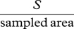
Margalef's index	DMg
Menhinick's index	DMn
proportional abundance indices
Shannon–Weiner index	H′		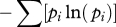rare species
inverse Simpson's index	D		common species
Pielou's index	HP		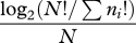rare species
Brillouin index	HB		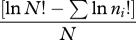rare species
McIntosh's U index	U		rare species
McIntosh's D index	D		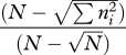common species
Berger–Parker index	d		common species
Cuba's index	DC		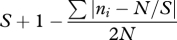common species
Q-statistic	Q		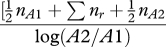rare species
evenness indices
Shannon evenness	J
Brillouin evenness	EB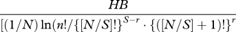
McIntosh evenness	EU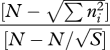

Despite the existence of the unifying concept of diversity, disagreement still exists among ecologists on how to conceptualize and evaluate species diversity [46]. Various attempts to unambiguously define species diversity have been tried [47–49], with some claiming that it is impossible [19,50]. As with diversity, many measures of evenness exist but there is no agreement on which is preferred [51,52], despite its relevance for ecosystem stability and functioning [53]. Recently, Ricotta [49], based on work by Juhasz–Nagy [54], classified diversity indices into four basic families: (i) richness diversity, (ii) evenness diversity, (iii) differentiation diversity, and (iv) abundance-weighted diversity. This classification requires three basic elements: (i) the number of species within an assemblage (R), (ii) the abundance distribution among species within an assemblage [20], and (iii) a measure of differences in species composition among subunits within that assemblage.

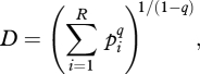
The recent work by Jost [55] and Tuomisto [38] provides a framework to integrate the previous concepts into a consistent terminology, based on the paper by Hill [56]. This formulation, based on numbers equivalents, unifies the three most popular diversity metrics (the number of species, the Shannon–Weiner index and the Simpson index) as special cases of the general index of diversity:

3.1

where R is the number of species, p_i is the frequency of the ith species and q is a parameter that determines how species frequencies are weighted [56]. When q = 0, D = R, i.e. species richness; when q = 1, D becomes the exponential Shannon–Weiner index and when q = 2, D becomes the inverse of the Simpson index. For these indices, evenness is E = D/R, or equivalently, diversity is the product of richness and evenness (D = R×E).

(b). Spatial scale

One difference between ecological and geographical perspectives is spatial and temporal extent (table 1). In addition to differences in extent, biogeographic studies often use larger grain sizes (e.g. 10 × 10 km blocks) than ecological ones (e.g. 1 × 1 m quadrats). The effect of spatial scale on species diversity is one of the oldest topics in ecology and biogeography [57,58]. However, spatial scale is not simply represented by increasing area, but also by interactions among the different scale components: grain, focus and extent [59,60].

A challenge in measuring species diversity is to account for the effects of scale. The idea of partitioning diversity into spatial (by analogy also temporal) components was introduced by Whittaker [61] and labelled α-diversity and γ-diversity, namely species diversity measured at community and landscape extents, respectively. Whittaker later [18] expanded that hierarchy to include point diversity (diversity within a community) and δ-diversity (diversity of a region). Unfortunately, the meaning of each of those levels was never made explicit. Jost [62] and Tuomisto [63] recently proposed focusing on just two units divorced of any explicit spatial or temporal scale: γ-diversity (D_γ), the total species diversity of a set of samples, and α-diversity (D_α), the mean species diversity of the individual samples. This collapsing of the basic measures of diversity untangles scale and diversity, permitting explicit and separate analyses of scale effects on diversity, and reunites ecological and biogeographic perspectives by permitting diversity to be conceptualized and measured similarly in both disciplines.

Moreover, Toumisto [63] resolved confusion about another measure of diversity introduced by Whittaker in 1960: β-diversity. A huge variety of measures of β-diversity have been proposed within three broad categories: the ratio of regional and local diversities, the difference in regional and local diversities where that difference can be absolute or proportional, and differences in species composition among samples [64–68]. Of those, the first provides a measure that has clear ecological meaning, the effective number of sampling units (e.g. communities) in a set of samples [55,56,62,63,69], where the ‘effective number’ is the number of sampling units necessary to contain the total diversity (D_γ) given that each unit consists of a set of unique species each with a mean diversity equal to D_α. Differentiation diversity is then:

3.2

These measures can then be combined with that of evenness [38]. The evenness of an entire set of samples is:

3.3

where R_γ = D_γ for q = 0; this index is contained in the interval [0,1]. Note, however, that R_α, the mean species richness of the individual samples, equals D_α for q = 0 only when each species has the same abundance in all samples. As a result E_α = D_α/R_α can be greater than unity. Finally, we can define β-richness as:

3.3

and β-evenness as:

3.4

In this framework, the concepts of diversity, richness, evenness and differentiation are all combined into a single scale-free formulation with a multiplicative relationship among them. Most of the other indices of diversity and evenness are derivable within this framework [63,70]. Of course, the grain, focus and extent by which a particular assemblage are measured matters, because changing the scale of the local community amounts to changing the scale at which the heterogeneity of the interactions between organisms and their environment manifests itself, resulting in a different balance between α-, β- and γ-diversity [71]. As a consequence, study design and spatial scales need to be explicitly stated.

Despite the existence of this theoretical framework, problems still exist in applying and modelling species diversity data at larger scales, especially for issues connected to the use of abundance data. Species diversity data are often both limited in the area sampled and do not include measures of abundance. However, while the effects of scale on species richness are known and modelled [72,73], the same effects on evenness have been little studied [74], largely because of practical limitations in measuring abundance. As a consequence, species diversity data at larger scales are usually restricted to species richness information.

The effects of how changing q can affect estimates of diversity components and how those change with spatial extent can be understood by considering some empirical data (table 3). The data consist of a floristic survey of the Natura 2000 Network of protected areas (PAs) in Siena Province. The individual PAs varied from 8.3 to 94.6 km² scattered over an extent of 3820 km² (for details see [15]). The survey consisted of 219 plots of 10 × 10 m (one per square-kilometre). Abundance was measured as the frequency of each species in 16 subplots within each plot. A total of 778 plant species were observed. For q = 0, the ratios of diversity at the grain of each protected area and entire network to that of each individual plot (effective number of sampling units [63]) was 8.6 and 27.6, respectively. In contrast, for q = 2, the ratios are 3.7 and 6.6, with intermediate values for q = 1. That is, at the plot scale, diversity of abundant species is captured to a much greater extent than rare species. Similarly, variation among units as measured by β-diversity is greater for q = 0 than q = 2, especially among plots within protected areas. Depending on the goals regarding diversity preservation of abundant and/or rare species, these differences in diversity patterns could lead to different management strategies.

Table 3.

An example of diversity partitioning across different spatial components for floristic data from a set of plots within protected areas of the Natura 2000 Network in Siena Province. The different spatial components are: the mean α-diversity among all plots (α_Plot), the mean β-diversity among plots within protected areas (β_PA), the mean α- and β-diversity among protected areas within the entire network (α_PA and β_Network, respectively) and γ-diversity of the whole network (γ_Network).

	D
spatial component	q = 0	q = 1	q = 2
αPlot	28.20	21.22	17.95
βPA	8.60	5.33	3.71
αPA	242.54	113.19	66.72
βNetwork	3.21	2.18	1.78
γNetwork	778	246.80	119.08

(c). Not all the species are the same

An important limitation of diversity measures is that not all species are functionally, evolutionarily and ecologically equivalent. Traditional measures of species diversity fail to capture this variation. Vane-Wright et al. [75] suggested that phylogenetic relationships among species should be included in diversity measures. They proposed a measure of taxonomic distinctiveness based on the geometry of a taxonomic tree.

This phylogenetic diversity is defined as the sum of the lengths of the branches of a phylogenetic tree that connects all the taxa present in a sample ([76], see also [23]). As functional and ecological traits of species are the result of evolution, a positive relationship between species' phylogenetic distances and ecological dissimilarity is expected assuming niche conservatism [76,77]. An overall measure of phylogenetic distances among species within a community, thus, can provide an index of biodiversity which captures information about trait and functional variation. Communities composed of species spanning a greater proportion of a phylogenetic tree are more diverse because those species are likely to have different ecological functions, or similar functions achieved through different phylogenetic patterns [75,78].

Many measures of phylogenetic diversity have been proposed, on the basis either of the distance among nodes or of branch lengths [75,79–82]. As is the case for species diversity indices, phylogenetic diversity measures use a variety of distance-based and topology-based indices [83], with disagreements about which indices provide the best measures.

Similar to the definition of D (see §3a), Pavoine et al. [84] proposed a parametric metric, I_q, where selected values of q correspond to classical indices of phylogenetic diversity. When q = 0, I₀ equals Faith's PD [80] minus the height of the phylogenetic tree [84]. When q = 1, I₁ equals the Shannon phylogenetic entropy of Allen et al. [85]. When q = 2, I₂ equals Rao's quadratic entropy [86], expressing the mean phylogenetic distance between two randomly chosen individuals in the community.

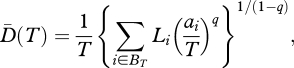
For conservation purposes, protected areas should not only capture current diversity, but also maintain diversity in the face of future possible losses. To establish a reserve network that contains a phylogenetically diverse set of species able to maintain total diversity, we need a metric able to indicate whether diversity is mostly in rare species that are more likely to go extinct. Such metrics should capture both abundance and phylogenetic information, and provide a measure of evenness. Recently, Cadotte & Davies [87] argued that prioritizing hotspots by incorporating evolutionary diversity metrics into prioritization schemes can help assess the conservation values of different regions based on evolutionary information. Using the approach of Chao et al. [88], phylogenetic information can be integrated into diversity measures based on Hill numbers (equation (3.1)). For a phylogenetic tree in which branch lengths are proportional to divergence times and branch tips are the same distance from the tree base (such a phylogenetic tree is defined as ultrametric and has useful mathematical properties, see Chao et al. [88]), the mean effective number of species (or lineages) over T years is:

3.5

where B_T denote the set of all branches in the time interval T, L_i represents the length (duration) of branch i in the set B_T and a_i is the total abundance of species on branch i. This diversity can be viewed as the effective number of maximally distinct lineages (or species) in the interval [−T,0] (with 0 representing the present time and −T a given past reference time). From another point of view, phylogenetic diversity of order q through T years ago can be defined as the product of the interval duration T, and the mean diversity over that interval, namely . For a set of maximally distinct species, all branch lengths equal T and reduces to Hill diversity D and, if q = 0, to R.

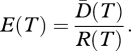
Similarly, a measure of phylogenetic evenness E(T) can be defined to express the extent to which a set of species are equally related through time period T. Following our previous rationale:

3.6

Low values of E(T) would indicate a set of species where most are closely related and a few are more distantly related. In contrast, for q = 0, E = 1 when the data consist of the maximal possible phylogenetic diversity through the considered T period. In a recent paper, Cadotte et al. [89] developed an entropic index of phylogenetic diversity based on an index of abundance-weighted evolutionary distinctiveness. In their approach, equitability (or evenness) could be obtained as the ratio between entropy and the number of species (logarithmically transformed). The phylogenetic evenness measure of Cadotte et al. [89] represents a special case of our more general parametric phylogenetic evenness (equation (3.6)). Communities with high values of and E(T) thus consist of species which are phylogenetically diverse, with that diversity spread across many of the common species, so that diversity is likely to be maintained in the face of future losses.

In recent decades, phylogenetic diversity has been analysed mostly for its implications in conservation biology [80,81,90,91]. Analyses at biogeographic scales are scarce, probably because of the difficulties in obtaining complete phylogenetic trees for a large number of species, even if data are becoming available for global scale analyses (see [23]).

4. Measuring species diversity in the real world

The growing impact of human activities on natural ecosystems requires urgent development of programmes for biodiversity assessment and monitoring [12,92], but standard methods are missing. Ideally, we would need data collected: (i) across relatively large spatial extents; (ii) within relatively short time-windows; and (iii) with the highest possible quality. Basically, we need data collected with an ecological lens across spatial extents typical of a biogeographic lens. However, assessment and monitoring of species diversity across such extents are constrained by limitations in our ability to accurately measure that diversity. Problems also arise from political and financial issues, but that topic is beyond the scope of this paper. Instead, we focus on scientific and practical barriers. We review these issues, with a special attention to explicitly contrasting ecological and biogeographic scales.

(a). Limitations in assessing species richness

One of the major limitations in assessing species diversity at biogeographic extents is because of problems in measuring species richness. Ideally, such an assessment would include the complete enumeration of the species within an area. Often, though, it is logistically infeasible to completely survey a large area so rare species are probably missed [93,94]. One solution is to use species richness estimators. A variety of estimation techniques exist, grouped into two main classes: extrapolation of species richness relationships (SRRs) [17,73] and using data about species occurrence and abundance within a sample. Extrapolation of SRRs is based on one of the most consistent relationships in ecology: increasing species richness with area or sampling intensity [57,58,95,96]. An SRR represents the way in which the number of species varies as a function of the space or time over which it is sampled. Evidence suggests the existence of scaling relationships in SRRs, with the slope of the curve changing with spatial scale [97]. Although we know something about the effects of scale components (sampling unit, grain, focus and extent) on SRRs, a general model does not exist [73,96,98,99]. The extrapolation of SRRs within ecological scales has been investigated, but this is typically limited to one to two orders of magnitude difference between the sampled area and the area of the estimate [17,73,100,101]. Much less is known about bias, accuracy and precision of SRRs when attempting to extrapolate far beyond the sampled area, the kind of extrapolation necessary for assessment at biogeographic extents.

The use of SRRs for estimating species richness has different implications for sampling designs at ecological and biogeographic scales. At ecological scales, the data typically consist of standard survey units (e.g. quadrats, traps) that are likely to consist of (supposedly) complete species lists and may also contain information on species abundances. Typically such units are arrayed in a regular, random or stratified-random design and the number of sample units can be large. In contrast, at biogeographic extents, sampling units are more often political or geographic entities for which species lists were obtained by heterogeneous sources, such as surveys, herbaria records and range distributions. As a result, the data used for SRRs at biogeographic scales are likely to be much less accurate. Research is needed on how to incorporate such data uncertainty into SRRs, possibly through the use of Bayesian estimators. It may be possible to devise sampling schemes that will provide accurate biodiversity estimates at less than continental extents, but research is needed. For example, should one use a greater number of sampling units of smaller size or a lesser number of larger size? For a given area sampled, a greater number of smaller sampling units provides higher total species richness in comparison with a lesser number of larger ones [94,98], but there are greater costs associated with such a sampling.

The other class of methods for estimating species richness is based on numbers of rare species or the species abundance distribution. The underlying concept is that the number of observed rare species provides an estimate of the number of unobserved species. In this case, ‘rare’ refers to species for which just one or two individuals were counted (‘singletons’ and ‘doubletons’), or which occurred in just one or two sampling units (‘uniques’ and ‘duplicates’). Examples of non-parametric estimators include the first- and second-order Jackknife [102–104], and the various Chao estimators [105,106]. Other estimators are based on the entire species abundance distribution, such as the bootstrap estimator [102,104,107]. Even at ecological scales, such as within a single stand of vegetation, these estimators are not free of bias [108], and little exploration of potential bias has been done at biogeographic scales. At intermediate extents, such as within a nature reserve or a region, the area surveyed can be less than 0.1–2% of the total area (e.g. [109,110]); in such cases, many rare species are missed, rendering non-parametric estimators ineffective [111]. The use of such estimators at biogeographic scales, such as a whole country or continent, may have an even greater probability of undersampling rare species [93]. New non-parametric estimators (e.g. [112]) might improve the performance of such methods, but a theoretical basis is still lacking. Thus, estimating species richness in an affordable way at biogeographic scales is not yet at hand.

Because of the problems in getting affordable data on the true total species richness, the R_γ of a region can only be assessed as the pooled species richness of a set of samples [38,55]. While this makes the definition of the R_γ of a region operational and objective, estimates of R_γ are always negatively biased with respect to the true richness and dependent on the number of sampling units. The same problem exists for estimates of R_β. Even temporal comparisons of total species richness may be difficult. One solution would be the establishment of well-defined, standardized sampling protocols, but it is unlikely that ecologists will ever agree on a single protocol and this may not be appropriate across different habitats and taxa. More difficult are comparisons based on different sampling schemes, which is highly likely at biogeographic extents or in monitoring temporal changes. Even at ecological scales within a network of collaborative projects, sampling protocols can differ [113]. Thus, methods for adjusting estimates to common scale components are needed. However, despite the well-known effects of sampling intensity on diversity estimates [114,115], many comparisons still fail to correct for differences in intensity (see [116]).

(b). Difficulties in getting adequate abundance data

Species-abundance distributions have been investigated with regard to niche differentiation, dispersal, speciation, density dependence and extinction [117,118]. In conservation biology, knowledge of the species-abundance distributions is used to predict the probability of population persistence or community stability in the face of global change [119].

Despite the theoretical and practical importance of species-abundance distributions, it is difficult to directly measure the abundance of all species at biogeographic extents. Estimators for evenness at large extents do not exist, and are likely to prove elusive, because of the difficulties in estimating the abundance of rare species. As a result, the assessment of evenness, while feasible at ecological scales, is almost impossible at biogeographic scales. Overcoming this hurdle requires understanding the relationship between the underlying species-abundance distribution of a large, regional community and the observed abundance distribution of a limited sample. Few have attempted to estimate species abundances at large spatial extents. Green & Plotkin [119] derived theoretical species-abundance distributions at regional scales as functions of sample size and the degree of conspecific spatial aggregation. Assuming populations are randomly distributed, the locally sampled and regional-scale species-abundance distributions had the same functional form. However, deviations from this pattern occurred when populations were spatially aggregated, which is likely for most taxa. Further research is needed on leveraging abundance and aggregation patterns at local scales for predicting species regional patterns.

Species abundance can be measured in various ways depending on the taxon or the ecological question. The most intuitive measure of species abundance is the number of individuals. However, while this is relatively common and easy for taxa such as birds, fish or woody plants, this measure has severe logistical limitations for clonal or tiny taxa (e.g. corals, grasses, mosses and lichens) especially at biogeographic spatial extents; alternative measures such as per cent cover or biomass may be used. While such measures do not pose a problem when used in isolation, measures obtained with one measure of abundance differ greatly from those obtained using another measure [120], making it important that study designs are clearly described [68,73].

As a general rule, most species are rare, either because of low abundance or because they are found in rare habitats [121,122]. Despite the potential importance of rare species for community stability [123], such species are difficult to assess at large spatial and temporal extents, necessitating greater sampling efforts. As a consequence, data collected at large extents may under-represent rare species. Although occurrence and abundance are generally positively correlated, occurrence–abundance correlations are dependent on the scale of measurement; for example, local plot abundances of breeding birds in eastern North America are independent of the spatial extent of the species [124]. In addition, occurrence–abundance correlation breaks down for habitat specialists [122]. On the other hand, spatial distributions are also extremely important for conservation biology. Occupancy-frequency distributions have been modelled to explain the relative abundance of core and satellite species [125]. This type of data might provide accurate estimates of species evenness, although this needs further investigation. Because species frequencies depend on the grain and extent of the sample [125,126], comparisons of such estimates collected with different sampling designs might be difficult. So, in analogy with species richness, evenness measures obtainable at larger spatial extents depend on the sampling design and may be inaccurate. Ricklefs [127] argued that ecologists should focus more on the distributions of populations in regions rather than on plots. Although this might not be practical, it provides a more natural underlying structure for distribution and abundance to which biodiversity measures could be related.

(c). Taxonomy and identification

In calculating any species diversity metric, it is assumed (implicitly or not) that all of the species in a sample or dataset have been properly identified and represent comparable units [128]. However, at least two types of problem affect this practice, one connected to taxonomic and nomenclature changes and a second connected to taxon identification and data management.

Updates in systematics and taxonomy can involve changes across nodes in the tree of life, from subpecies to phyla, and the pace of such changes is increasing. Such changes can create problems for estimates of species richness at both ecological and biogeographic scales, but especially the latter. One problem is how many species are actually in a sample. Molecular techniques can both reveal unrecognized species and collapse previously delineated groups [129,130]. The speed at which this is occurring can affect the accuracy of species richness estimates, especially when compared with historical records. Such taxonomic changes have more limited effects on measures of diversity which incorporate abundance data (equation (3.1)) as they are less sensitive to changes in rare species, but they can significantly affect taxonomic and phylogenetic measures of diversity (equation (3.5)).

Further problems come with attempts to synthesize surveys collected by different workers if they used different species concepts for the same group of individuals. This can be especially problematic for data collected in different decades, with the greatest problems created by the splitting of a single taxon into multiple units. These reclassifications affect research on change over time and at biogeographic scales when data are aggregated over many surveys. At minimum, species surveys must specify which taxonomic treatises are used. Changes in species classifications affect conservation efforts either by reducing conservation units to subspecies status or by inflating the potential number of conservation units through the splitting of taxa [131].

The problem connected with specimen identification is even more clear, as it deals with the human interpretation of assigning one object (e.g. an individual) to a category (e.g. a species). Although straightforward, this problem becomes manifest in diversity surveys. Ideally, one would voucher every identification for later checks or to account for changes in taxonomy. But such vouchering typically involves just one or a few specimens, with the assumption that all other individuals that were assessed as belonging to the same species were correctly identified. Nor is subsequent identification of specimens free from bias and re-identification of specimens might not be able to be transferred to the original (field) data and/or diversity estimations.

5. Conclusions

Based on the above discussed limitations on the assessment of biodiversity, the science of biodiversity badly needs a research agenda. Many improvements have been achieved to date, leading to better knowledge of biodiversity. In particular, genetic and genomic information, nowadays more and more available, has greatly enhanced classical surveys based on species richness and abundance through methods such as DNA barcoding [132,137].

Similarly, the assessment of phylogenetic diversity will be used more often for conservation planning, especially at larger spatial extents [23,133]. Recent advances in sequencing technologies are improving our capacity to easily incorporate phylogenetic information into diversity indices. This information has significantly advanced our understanding of historical patterns of biodiversity, phylogeography and biogeography, and can help inform current conservation strategies and future responses to global change [23,134]. Conservation priorities should take into account phylogeny, with areas containing greater phylogenetic differentiation given greater conservation priority [75,82,133].

With respect to classical biodiversity measures, we note an increasing interest of ecologists in expanding the analysis of diversity to the assessment of inventory (e.g. species richness) as well as differentiation diversity (e.g. β-diversity). In this way, we can determine how variation in community composition affects ecosystem function and services at landscape scales. Moreover, given the important role of spatial scale in the analysis of diversity patterns, theoretical frameworks to estimate the influence of spatial scale on biodiversity have been proposed, and the use of spatially explicit data is becoming common in ecology and biogeography [59]. This represents a critical step towards increasing our understanding on the effect of scale components on diversity measures.

Although estimates of abundance may not be available at large extents, analyses based on occupancy or occurrence alone may have their own intrinsic value; for example, indicator species analysis based on occupancy frequency can give important information for conservation actions [135]. In the same way, analyses of species co-occurrence or species nestedness could be performed at large spatial scales even if data on all species were limited to occurrence data.

Finally, standardized sampling procedures and large-scale cooperative programmes using standardized protocols are becoming well-established for collecting biodiversity data among the world's biomes. Conservation International recently launched the Tropical Ecology, Assessment, and Monitoring (TEAM) Initiative to establish a network of more than 50 field stations worldwide to assess and monitor biodiversity [136]. This initiative is a good example of how collaborative efforts of governments, non-governmental organizations and scientific societies can greatly improve biodiversity conservation and knowledge.

Although we are aware that further explorations are needed of bias, precision and accuracy of metrics of richness, evenness and phylogenetic diversity, we believe that these will be accomplished in the near future through the complementary use of computer simulations based on theoretical communities and empirical analyses of actual data (e.g. [102,107]). Biodiversity conservation and management requires predictive understanding of the role of diversity in ecosystem structure and function and the ways that global change might affect those relationships. Central to our understanding of those relationships is the measurement of biodiversity, particularly in ways that will allow us to take information at one scale and use it to produce knowledge at other scales. Ecological and biogeographic approaches to this issue provide different lenses from which to view the problem, each with its unique strengths and weaknesses. Even if biodiversity science is in its infancy, at least for applied topics, the combination of different perspectives will allow the necessary steps forward.

References

- 1.Wilson E. O., Peter F. M. 1981. Biodiversity. Washington, DC: National Academy Press [Google Scholar]
- 2.Scheiner S. M., Willig M. R. 2011. The theory of ecology. Chicago, IL: University of Chicago Press [Google Scholar]
- 3.Butchart S. H. M., et al. 2010. Global biodiversity: indicators of recent declines. Science 328, 1164–1168 10.1126/science.1187512 (doi:10.1126/science.1187512) [DOI] [PubMed] [Google Scholar]
- 4.Hector A., Bagchi R. 2007. Biodiversity and ecosystem multifunctionality. Nature 448, 188–190 10.1038/nature05947 (doi:10.1038/nature05947) [DOI] [PubMed] [Google Scholar]
- 5.Hector A. 1998. The effect of diversity on productivity: detecting the role of complementarity. Oikos 82, 597–599 10.2307/3546380 (doi:10.2307/3546380) [DOI] [Google Scholar]
- 6.Loreau M., Naeem S., Inchausti P. (eds) 2002. Biodiversity and ecosystem functioning: synthesis and perspectives. Oxford, UK: Oxford University Press [Google Scholar]
- 7.Naeem S., Bunker D. E., Hector A. 2009. Biodiversity, ecosystem functioning, and human wellbeing: an ecological and economic perspective. Oxford, UK: Oxford University Press [Google Scholar]
- 8.Baillie J. E. M., et al. 2008. Toward monitoring global biodiversity. Conserv. Lett. 1, 18–26 10.1111/j.1755-263X.2008.00009.x (doi:10.1111/j.1755-263X.2008.00009.x) [DOI] [Google Scholar]
- 9.Green R., Balmford A., Crane P., Mace G., Reynolds J., Turner R. 2005. A framework for improved monitoring of biodiversity: responses to the world summit on sustainable development. Conserv. Biol. 19, 56–65 10.1111/j.1523-1739.2005.00289.x (doi:10.1111/j.1523-1739.2005.00289.x) [DOI] [Google Scholar]
- 10.Duro D., Coops N., Wulder M., Han T. 2007. Development of a large area biodiversity monitoring system driven by remote sensing. Prog. Phys. Geogr. 31, 235–260 10.1177/0309133307079054 (doi:10.1177/0309133307079054) [DOI] [Google Scholar]
- 11.Henry P., et al. 2008. Integrating ongoing biodiversity monitoring: potential benefits and methods. Biodivers. Conserv. 17, 3357–3382 10.1007/s10531-008-9417-1 (doi:10.1007/s10531-008-9417-1) [DOI] [Google Scholar]
- 12.Pereira H., Cooper H. 2006. Towards the global monitoring of biodiversity change. Trends Ecol. Evol. 21, 123–129 10.1016/j.tree.2005.10.015 (doi:10.1016/j.tree.2005.10.015) [DOI] [PubMed] [Google Scholar]
- 13.Noss R. 1999. Assessing and monitoring forest biodiversity: a suggested framework and indicators. For. Ecol. Manage. 115, 135–146 10.1016/S0378-1127(98)00394-6 (doi:10.1016/S0378-1127(98)00394-6) [DOI] [Google Scholar]
- 14.Feld C., et al. 2009. Indicators of biodiversity and ecosystem services: a synthesis across ecosystems and spatial scales. Oikos 118, 1862–1871 10.1111/j.1600-0706.2009.17860.x (doi:10.1111/j.1600-0706.2009.17860.x) [DOI] [Google Scholar]
- 15.Chiarucci A., Bacaro G., Rocchini D. 2008. Quantifying plant species diversity in a Natura 2000 network: old ideas and new proposals. Biol. Conserv. 141, 2608–2618 10.1016/j.biocon.2008.07.024 (doi:10.1016/j.biocon.2008.07.024) [DOI] [Google Scholar]
- 16.Feld C. K., Sousa J. P., Silva P. M., Dawson T. P. 2010. Indicators for biodiversity and ecosystem services: towards an improved framework for ecosystems assessment. Biodivers. Conserv. 19, 2895–2919 10.1007/s10531-010-9875-0 (doi:10.1007/s10531-010-9875-0) [DOI] [Google Scholar]
- 17.Colwell R., Coddington J. 1994. Estimating terrestrial biodiversity through extrapolation. Phil. Trans. R. Soc. Lond. B 345, 101–118 10.1098/rstb.1994.0091 (doi:10.1098/rstb.1994.0091) [DOI] [PubMed] [Google Scholar]
- 18.Whittaker R. H. 1972. Evolution and measurement of species diversity. Taxon 21, 213–251 10.2307/1218190 (doi:10.2307/1218190) [DOI] [Google Scholar]
- 19.Hurlbert S. H. 1971. The nonconcept of species diversity: a critique and alternative parameters. Ecology 52, 577–586 10.2307/1934145 (doi:10.2307/1934145) [DOI] [PubMed] [Google Scholar]
- 20.Peet R. 1974. The measurement of species diversity. Ann. Rev. Ecol. Syst. 5, 285–307 10.1146/annurev.es.05.110174.001441 (doi:10.1146/annurev.es.05.110174.001441) [DOI] [Google Scholar]
- 21.Ellison A. 2010. Partitioning diversity. Ecology 91, 1962–1963 10.1890/09-1692.1 (doi:10.1890/09-1692.1) [DOI] [PubMed] [Google Scholar]
- 22.Brown J. H., Maurer B. A. 1989. Macroecology: the division of food and space among species on continents. Science 243, 1145–1150 10.1126/science.243.4895.1145 (doi:10.1126/science.243.4895.1145) [DOI] [PubMed] [Google Scholar]
- 23.Davies J., Buckley L. B. 2011. Phylogenetic diversity as a window into the evolutionary and biogeographic histories of present-day richness gradients for mammals. Phil. Trans. R. Soc. B 366, 2414–2425 10.198/rstb.2011.0058 (doi:10.198/rstb.2011.0058) [DOI] [PMC free article] [PubMed] [Google Scholar]
- 24.MacArthur R. H., Wilson E. O. 1967. The theory of island biogeography. Princeton, NJ: Princeton University Press [Google Scholar]
- 25.Sax D., Gaines S. 2011. The equilibrium theory of island biogeography. In The theory of ecology, pp. 219–240 Chicago, IL: Chicago University Press [Google Scholar]
- 26.Scheiner S., Willig M. 2011. A general theory of ecology. In The theory of ecology, pp. 3–18 Chicago, IL: University of Chicago Press [Google Scholar]
- 27.Wiens J., Donoghue M. 2004. Historical biogeography, ecology and species richness. Trends Ecol. Evol. 19, 639–644 10.1016/j.tree.2004.09.011 (doi:10.1016/j.tree.2004.09.011) [DOI] [PubMed] [Google Scholar]
- 28.Kreft H., Jetz W., Mutke J., Kier G., Barthlott W. 2008. Global diversity of island floras from a macroecological perspective. Ecol. Lett. 11, 116–127 [DOI] [PubMed] [Google Scholar]
- 29.Willig M., Bloch C. 2006. Latitudinal gradients of species richness: a test of the geographic area hypothesis at two ecological scales. Oikos 112, 163–173 10.1111/j.0030-1299.2006.14009.x (doi:10.1111/j.0030-1299.2006.14009.x) [DOI] [Google Scholar]
- 30.Wilson J., Wells T., Trueman I., Jones G., Atkinson M., Crawley M., Dodd M. E., Silvertown J. 1996. Are there assembly rules for plant species abundance? An investigation in relation to soil resources and successional trends. J. Ecol. 84, 527–538 10.2307/2261475 (doi:10.2307/2261475) [DOI] [Google Scholar]
- 31.Tilman D., Reich P., Knops J. 2006. Biodiversity and ecosystem stability in a decade-long grassland experiment. Nature 441, 629–632 10.1038/nature04742 (doi:10.1038/nature04742) [DOI] [PubMed] [Google Scholar]
- 32.Polley H., Wilsey B., Derner J. 2003. Do species evenness and plant density influence the magnitude of selection and complementarity effects in annual plant species mixtures? Ecol. Lett. 6, 248–256 10.1046/j.1461-0248.2003.00422.x (doi:10.1046/j.1461-0248.2003.00422.x) [DOI] [Google Scholar]
- 33.Robinson G., Yurlina M., Handel S. 1994. A century of change in the Staten Island flora: ecological correlates of species losses and invasions. Bull. Torrey Botanical Club 121, 119–129 10.2307/2997163 (doi:10.2307/2997163) [DOI] [Google Scholar]
- 34.McCollin D., Moore L., Sparks T. 2000. The flora of a cultural landscape: environmental determinants of change using archival sources. Biol. Conserv. 92, 249–263 10.1016/S0006-3207(99)00070-1 (doi:10.1016/S0006-3207(99)00070-1) [DOI] [Google Scholar]
- 35.Mouillot D., Wilson J. 2002. Can we tell how a community was constructed? A comparison of five evenness indices for their ability to identify theoretical models of community construction. Theoret. Popul. Biol. 61, 141–151 10.1006/tpbi.2001.1565 (doi:10.1006/tpbi.2001.1565) [DOI] [PubMed] [Google Scholar]
- 36.Chiarucci A., Alongi C., Wilson J. B. 2004. Competitive exclusion and the no-interaction model operate simultaneously in microcosm plant communities. J. Veget. Sci. 15, 789–796 [Google Scholar]
- 37.Mulder C., Bazeley-White E., Dimitrakopoulos P., Hector A., Scherer-Lorenzen M., Schmid B. 2004. Species evenness and productivity in experimental plant communities. Oikos 107, 50–63 10.1111/j.0030-1299.2004.13110.x (doi:10.1111/j.0030-1299.2004.13110.x) [DOI] [Google Scholar]
- 38.Tuomisto H. 2010. A consistent terminology for quantifying species diversity? Yes, it does exist. Oecologia 164, 853–860 10.1007/s00442-010-1812-0 (doi:10.1007/s00442-010-1812-0) [DOI] [PubMed] [Google Scholar]
- 39.Palmer M. W., White P. S. 1994. On the existence of ecological communities. J. Veget. Sci. 5, 279–282 10.2307/3236162 (doi:10.2307/3236162) [DOI] [Google Scholar]
- 40.Chiarucci A. 2007. To sample or not to sample? That is the question … for the vegetation scientist. Folia Geobot. 42, 209–216 10.1007/BF02893887 (doi:10.1007/BF02893887) [DOI] [Google Scholar]
- 41.Magurran A. E. 2004. Measuring biological diversity. Malden, MA: Blackwell Science [Google Scholar]
- 42.Gurevitch J., Scheiner S. M., Fox G. A. 2006. The ecology of plants,. Sunderland, MA: Sinauer Associates [Google Scholar]
- 43.Laffan S. W., Lubarsky E., Rosauer D. F. 2010. Biodiverse, a tool for the spatial analysis of biological and related diversity Ecography 33, 643–647 10.1111/j.1600-0587.2010.06237.x (doi:10.1111/j.1600-0587.2010.06237.x) [DOI] [Google Scholar]
- 44.Shannon C. E. 1948. A mathematical theory of communication. Bell Syst. Tech. J. 27, 379–423 623–656 [Google Scholar]
- 45.Simpson E. H. 1949. Measurement of diversity. Nature 163, 688–688 10.1038/163688a0 (doi:10.1038/163688a0) [DOI] [Google Scholar]
- 46.Ricotta C. 2005. Through the jungle of biological diversity. Acta Biotheoret. 53, 29–38 10.1007/s10441-005-7001-6 (doi:10.1007/s10441-005-7001-6) [DOI] [PubMed] [Google Scholar]
- 47.Solow A. R., Polasky S. 1994. Measuring biological diversity. Environ. Ecol. Stat. 1, 95–103 10.1007/BF02426650 (doi:10.1007/BF02426650) [DOI] [Google Scholar]
- 48.Sarkar S., Margules C. 2002. Operationalizing biodiversity for conservation planning. J. Biosci. 27, 299–308 10.1007/BF02704961 (doi:10.1007/BF02704961) [DOI] [PubMed] [Google Scholar]
- 49.Ricotta C. 2007. A semantic taxonomy for diversity measures. Acta Biotheoret. 55, 23–33 10.1007/s10441-007-9008-7 (doi:10.1007/s10441-007-9008-7) [DOI] [PubMed] [Google Scholar]
- 50.Poole R. W. 1974. An introduction to quantitative ecology. New York, NY: McGraw-Hill [Google Scholar]
- 51.Smith B., Wilson J. 1996. A consumer's guide to evenness indices. Oikos 76, 70–82 10.2307/3545749 (doi:10.2307/3545749) [DOI] [Google Scholar]
- 52.Jost L. 2010. The relation between evenness and diversity. Diversity 2, 207–232 10.3390/d2020207 (doi:10.3390/d2020207) [DOI] [Google Scholar]
- 53.Wittebolle L., Marzorati M., Clement L., Balloi A., Daffonchio D., Heylen K., De Vos P., Verstraete W., Boon N. 2009. Initial community evenness favours functionality under selective stress. Nature 458, 623–626 10.1038/nature07840 (doi:10.1038/nature07840) [DOI] [PubMed] [Google Scholar]
- 54.Juhász-Nagy P. 1993. Notes on compositional diversity. Hydrobiologia 249, 173–182 10.1007/BF00008852 (doi:10.1007/BF00008852) [DOI] [Google Scholar]
- 55.Jost L. 2006. Entropy and diversity. Oikos 113, 363–375 10.1111/j.2006.0030-1299.14714.x (doi:10.1111/j.2006.0030-1299.14714.x) [DOI] [Google Scholar]
- 56.Hill M. O. 1973. Diversity and evenness: a unifying notation and its consequences. Ecology 54, 427–432 10.2307/1934352 (doi:10.2307/1934352) [DOI] [Google Scholar]
- 57.Arrhenius O. 1921. Species and area. J. Ecol. 9, 95–99 10.2307/2255763 (doi:10.2307/2255763) [DOI] [Google Scholar]
- 58.Gleason H. A. 1922. On the relation between species and area. Ecology 3, 158–162 10.2307/1929150 (doi:10.2307/1929150) [DOI] [Google Scholar]
- 59.Dungan J. L., Perry J. N., Dale M. R. T., Legendre P., Citron-Pousty S., Fortin M. J., Jakomulska A., Miriti M., Rosemberg M. S. 2002. A balanced view of scale in spatial statistical analysis. Ecography 25, 626–640 10.1034/j.1600-0587.2002.250510.x (doi:10.1034/j.1600-0587.2002.250510.x) [DOI] [Google Scholar]
- 60.Scheiner S. M. 2003. Six types of species–area curves. Glob. Ecol. Biogeogr. 12, 441–447 10.1046/j.1466-822X.2003.00061.x (doi:10.1046/j.1466-822X.2003.00061.x) [DOI] [Google Scholar]
- 61.Whittaker R. H. Vegetation of the Siskiyou Mountains, Oregon and California. Ecol. Monogr. 30, 279–338 10.2307/1943563 (doi:10.2307/1943563) [DOI] [Google Scholar]
- 62.Jost L. 2007. Partitioning diversity into independent alpha and beta components. Ecology 88, 2427–2439 10.1890/06-1736.1 (doi:10.1890/06-1736.1) [DOI] [PubMed] [Google Scholar]
- 63.Tuomisto H. 2010. A diversity of beta diversities: straightening up a concept gone awry. I. Defining beta diversity as a function of alpha and gamma diversity. Ecography 33, 2–22 10.1111/j.1600-0587.2009.05880.x (doi:10.1111/j.1600-0587.2009.05880.x) [DOI] [Google Scholar]
- 64.Scheiner S. M. 1992. Measuring pattern diversity. Ecology 73, 1860–1867 10.2307/1940037 (doi:10.2307/1940037) [DOI] [Google Scholar]
- 65.Vellend M. 2001. Do commonly used indices of β-diversity measure species turnover? J. Veget. Sci. 12, 545–552 10.2307/3237006 (doi:10.2307/3237006) [DOI] [Google Scholar]
- 66.Jurasinski G., Retzer V., Beierkuhnlein C. 2009. Inventory, differentiation, and proportional diversity: a consistent terminology for quantifying species diversity. Oecologia 159, 15–26 10.1007/s00442-008-1190-z (doi:10.1007/s00442-008-1190-z) [DOI] [PubMed] [Google Scholar]
- 67.Koleff P., Gaston K. J., Lennon J. J. 2003. Measuring beta diversity for presence–absence data. J. Anim. Ecol. 72, 367–382 10.1046/j.1365-2656.2003.00710.x (doi:10.1046/j.1365-2656.2003.00710.x) [DOI] [Google Scholar]
- 68.Tuomisto H. 2010. A diversity of beta diversities: straightening up a concept gone awry. II. Quantifying beta diversity and related phenomena. Ecography 33, 23–45 10.1111/j.1600-0587.2009.06148.x (doi:10.1111/j.1600-0587.2009.06148.x) [DOI] [Google Scholar]
- 69.Baselga A. 2010. Multiplicative partition of true diversity yields independent alpha and beta components; additive partition does not. Ecology 91, 1974–1981 10.1890/09-0320.1 (doi:10.1890/09-0320.1) [DOI] [PubMed] [Google Scholar]
- 70.Jost L. 2010. Independence of alpha and beta diversities. Ecology 91, 1969–1974 10.1890/09-0368.1 (doi:10.1890/09-0368.1) [DOI] [PubMed] [Google Scholar]
- 71.Loreau M. 2000. Are communities saturated? On the relationship between alfa, beta and gamma diversity. Ecol. Lett. 3, 73–76 10.1046/j.1461-0248.2000.00127.x (doi:10.1046/j.1461-0248.2000.00127.x) [DOI] [Google Scholar]
- 72.Scheiner S. M., Cox S. B., Willig M., Mittelbach G. G., Osemberg C., Kaspari M. 2000. Species richness, species–area curves and Simpson's paradox. Evol. Ecol. Res. 2, 791–802 [Google Scholar]
- 73.Scheiner S. M., Chiarucci A., Fox G. A., Helmus M. R., McGlinn D. J., Willig M. R. 2011. The underpinnings of the relationship of species richness with space and time. Ecol. Monogr. 81, 195–213 [Google Scholar]
- 74.Wilson J. B., Steel J. B., King W. M., Gitay H. 1999. The effects of spatial scale on evenness. J. Veget. Sci. 10, 463–468 10.2307/3237181 (doi:10.2307/3237181) [DOI] [Google Scholar]
- 75.Vane-Wright R. I., Humphries C. J., Williams P. H. 1991. What to protect? Systematics and the agony of choice. Biol. Conserv. 55, 235–254 10.1016/0006-3207(91)90030-D (doi:10.1016/0006-3207(91)90030-D) [DOI] [Google Scholar]
- 76.Prinzing A. 2001. The niche of higher plants: evidence for phylogenetic conservatism. Proc. R. Soc. Lond. B 268, 2383–2389 10.1098/rspb.2001.1801 (doi:10.1098/rspb.2001.1801) [DOI] [PMC free article] [PubMed] [Google Scholar]
- 77.Gerhold P., Pärtel M., Liira J., Zobel K., Prinzing A. 2008. Phylogenetic structure of local communities predicts the size of the regional species pool. J. Ecol. 96, 709–712 10.1111/j.1365-2745.2008.01386.x (doi:10.1111/j.1365-2745.2008.01386.x) [DOI] [Google Scholar]
- 78.Faith D. P. 1996. Phylogenetic pattern and the quantification of organismal biodiversity. In Biodiversity. Measurement and estimation (ed. Hawksworth D. L.), pp. 45–57 London, UK: Chapman and Hall; [DOI] [PubMed] [Google Scholar]
- 79.Keith S. A., Newton A. C., Morecroft M. D., Bealey C. E., Bullock J. M. 2009. Taxonomic homogenization of woodland plant communities over 70 years. Proc. R. Soc. B 276, 3539–3544 10.1098/rspb.2009.0938 (doi:10.1098/rspb.2009.0938) [DOI] [PMC free article] [PubMed] [Google Scholar]
- 80.Faith D. P. 1992. Conservation evaluation and phylogenetic diversity. Biol. Conserv. 61, 1–10 10.1016/0006-3207(92)91201-3 (doi:10.1016/0006-3207(92)91201-3) [DOI] [Google Scholar]
- 81.Faith D. P. 1992. Systematics and conservation: on predicting the feature diversity of subsets of taxa. Cladistics 12, 361–373 10.1111/j.1096-0031.1992.tb00078.x (doi:10.1111/j.1096-0031.1992.tb00078.x) [DOI] [PubMed] [Google Scholar]
- 82.Keith M., Chimimba C. T., Reyers B., Jaarsveld A. S. 2005. Taxonomic and phylogenetic distinctiveness in regional conservation assessments: a case study based on extant South African Chiroptera and Carnivora. Anim. Conserv. 8, 279–288 10.1017/S1367943005002192 (doi:10.1017/S1367943005002192) [DOI] [Google Scholar]
- 83.Schweiger O., Klotz S., Durka W., Kühn I. 2008. A comparative test of phylogenetic diversity indices. Oecologia 157, 485–495 10.1007/s00442-008-1082-2 (doi:10.1007/s00442-008-1082-2) [DOI] [PubMed] [Google Scholar]
- 84.Pavoine S., Love M. S., Bonsall M. B. 2009. Hierarchical partitioning of evolutionary and ecological patterns in the organization of phylogenetically-structured species assemblages: application to rockfish (genus: Sebastes) in the Southern California Bight. Ecol. Lett. 12, 898–908 10.1111/j.1461-0248.2009.01344.x (doi:10.1111/j.1461-0248.2009.01344.x) [DOI] [PubMed] [Google Scholar]
- 85.Allen B., Kon M., Bar-Yam Y. 2009. A new phylogenetic diversity measure generalizing the Shannon Index and its application to Phyllostomid bats. Am. Nat. 174, 236–243 10.1086/600101 (doi:10.1086/600101) [DOI] [PubMed] [Google Scholar]
- 86.Rao C. R. 1982. Diversity and dissimilarity coefficients: a unified approach. Theoret. Popul. Biol. 21, 24–43 10.1016/0040-5809(82)90004-1 (doi:10.1016/0040-5809(82)90004-1) [DOI] [Google Scholar]
- 87.Cadotte M. W., Davies T. J. 2010. Rarest of the rare: advances in combining evolutionary distinctiveness and scarcity to inform conservation at biogeographical scales. Divers. Distrib. 16, 376–385 10.1111/j.1472-4642.2010.00650.x (doi:10.1111/j.1472-4642.2010.00650.x) [DOI] [Google Scholar]
- 88.Chao A., Chiu C., Jost L. 2010. Phylogenetic diversity measures based on Hill numbers. Phil. Trans. R. Soc. B 365, 3599–3609 10.1098/rstb.2010.0272 (doi:10.1098/rstb.2010.0272) [DOI] [PMC free article] [PubMed] [Google Scholar]
- 89.Cadotte M. W., Davies T. J., Regetz J., Kembel W. S., Cleland E., Oakley T. H. 2010. Phylogenetic diversity metrics for ecological communities: integrating species richness, abundance and evolutionary history. Ecol. Lett. 13, 96–105 10.1111/j.1461-0248.2009.01405.x (doi:10.1111/j.1461-0248.2009.01405.x) [DOI] [PubMed] [Google Scholar]
- 90.Crozier R. H., Dunnett L. J., Agapow P. 2005. Phylogenetic biodiversity assessment based on systematic nomenclature. Evol. Bioinformatics Online 1, 11–36 [PMC free article] [PubMed] [Google Scholar]
- 91.Faith D. P., Baker A. M. 2006. Phylogenetic diversity (PD) and biodiversity conservation: some bioinformatics challenges. Evol. Bioinformatics Online 2, 121–128 [PMC free article] [PubMed] [Google Scholar]
- 92.Pereira H. M., et al. 2010. Scenarios for global biodiversity in the 21st century. Science 330, 1496–1501 10.1126/science.1196624 (doi:10.1126/science.1196624) [DOI] [PubMed] [Google Scholar]
- 93.Palmer M. W. 1995. How should one count species? Natural Areas J. 15, 124–135 [Google Scholar]
- 94.Palmer M. W., Earls P. G., Hoagland B. W., White P. S., Wohlgemuth T. 2002. Quantitative tools for perfecting species lists. Environmetrics 13, 121–137 10.1002/env.516 (doi:10.1002/env.516) [DOI] [Google Scholar]
- 95.Connor E. F., McCoy E. D. 1979. The statistics and biology of the species-area relationship. Am. Nat. 113, 791–833 10.1086/283438 (doi:10.1086/283438) [DOI] [Google Scholar]
- 96.Palmer M. W., White P. S. 1994. Scale dependence and the species-area relationship. Am. Nat. 144, 717–740 10.1086/285704 (doi:10.1086/285704) [DOI] [Google Scholar]
- 97.Crawley M. J., Harral J. E. 2001. Scale dependence in plant biodiversity. Science 291, 864–868 10.1126/science.291.5505.864 (doi:10.1126/science.291.5505.864) [DOI] [PubMed] [Google Scholar]
- 98.Condit R., Hubbell S. P., Lafrankie J. V., Sukumar R., Manokaran R., Foster R. B., Ashton P. S. 1996. Species–area and species–individual relationships for tropical trees: a comparison of three 50-ha plots. J. Ecol. 84, 549–562 10.2307/2261477 (doi:10.2307/2261477) [DOI] [Google Scholar]
- 99.Chiarucci A., Bacaro G., Rocchini D., Ricotta C., Palmer M. W., Scheiner S. M. 2009. Spatially constrained rarefaction: incorporating the autocorrelated structure of biological communities into sample-based rarefaction. Commun. Ecol. 10, 209–214 10.1556/ComEc.10.2009.2.11 (doi:10.1556/ComEc.10.2009.2.11) [DOI] [Google Scholar]
- 100.Keating K. A., Quinn J. F. 1998. Estimating species richness: the Michaelis–Menten model revisited. Oikos 81, 411–416 10.2307/3547060 (doi:10.2307/3547060) [DOI] [Google Scholar]
- 101.Colwell R. K., Mao C. X., Chang J. 2004. Interpolating, extrapolating, and comparing incidence-based species accumulation curves. Ecology 85, 2717–2727 10.1890/03-0557 (doi:10.1890/03-0557) [DOI] [Google Scholar]
- 102.Heltshe J. F., Forrester N. E. 1983. Estimating species richness using the Jackknife procedure. Biometrics 39, 1–11 10.2307/2530802 (doi:10.2307/2530802) [DOI] [PubMed] [Google Scholar]
- 103.Burnham K. P., Overton W. S. 1978. Estimation of the size of a closed population when probabilities vary among animals. Biometrika 65, 625–633 10.1093/biomet/65.3.625 (doi:10.1093/biomet/65.3.625) [DOI] [Google Scholar]
- 104.Burnham K. P., Overton W. S. 1979. Robust estimation of population size when capture probabilities vary among animals. Ecology 60, 927–936 10.2307/1936861 (doi:10.2307/1936861) [DOI] [Google Scholar]
- 105.Chao A. 1984. Nonparametric-estimation of the number of classes in a population. Scand. J. Stat. 11, 265–270 [Google Scholar]
- 106.Chao A. 1987. Estimating the population size for capture-recapture data with unequal catchability. Biometrics 43, 783–791 10.2307/2531532 (doi:10.2307/2531532) [DOI] [PubMed] [Google Scholar]
- 107.Smith E. P., van Belle G. 1984. Nonparametric estimation of species richness. Biometrics 40, 119–129 10.2307/2530750 (doi:10.2307/2530750) [DOI] [Google Scholar]
- 108.Chiarucci A., Enright N. J., Perry G. L. W., Miller B. P., Lamont B. B. 2003. Performance of nonparametric species richness estimators in a high diversity plant community. Divers. Distrib. 9, 283–295 10.1046/j.1472-4642.2003.00027.x (doi:10.1046/j.1472-4642.2003.00027.x) [DOI] [Google Scholar]
- 109.Skov F., Lawesson J. 2000. Estimation of plant species richness from systematically placed plots in a managed forest ecosystem. Nord. J. Bot. 20, 477–483 10.1111/j.1756-1051.2000.tb01592.x (doi:10.1111/j.1756-1051.2000.tb01592.x) [DOI] [Google Scholar]
- 110.Chiarucci A., Maccherini S., De Dominicis V. 2001. Evaluation and monitoring of the flora in a nature reserve by estimation methods. Biol. Conserv. 101, 305–314 10.1016/S0006-3207(01)00073-8 (doi:10.1016/S0006-3207(01)00073-8) [DOI] [Google Scholar]
- 111.D'Alessandro L., Fattorini L. 2002. Resampling estimators of species richness from presence-absence data: why they don't work. Metron 61, 5–19 [Google Scholar]
- 112.Hwang W. H., Shen T. J. 2010. Small-sample estimation of species richness applied to forest communities. Biometrics 66, 1052–1060 10.1111/j.1541-0420.2009.01371.x (doi:10.1111/j.1541-0420.2009.01371.x) [DOI] [PubMed] [Google Scholar]
- 113.Gross K. L., Willig M. R., Gough L., Inouye R., Cox S. B. 2000. Patterns of species density and productivity at different spatial scales in herbaceous plant communities. Oikos 89, 417–427 10.1034/j.1600-0706.2000.890301.x (doi:10.1034/j.1600-0706.2000.890301.x) [DOI] [Google Scholar]
- 114.Sanders H. L. 1968. Marine benthic diversity: a comparative study. Am. Nat. 102, 243–282 10.1086/282541 (doi:10.1086/282541) [DOI] [Google Scholar]
- 115.Gollies N. J., Colwell R. W. 2001. Quantifying biodiversity: procedures and pitfalls in the measurement and comparison of species richness. Ecol. Lett. 4, 379–391 10.1046/j.1461-0248.2001.00230.x (doi:10.1046/j.1461-0248.2001.00230.x) [DOI] [Google Scholar]
- 116.Palmer M. W., McGlinn D. J., Fridley J. D. 2008. Artifacts and artifictions in biodiversity research. Folia Geobot. 43, 245–257 10.1007/s12224-008-9012-y (doi:10.1007/s12224-008-9012-y) [DOI] [Google Scholar]
- 117.Tokeshi M. 1993. Species abundance patterns and community structure. Adv. Ecol. Res. 24, 111–186 10.1016/S0065-2504(08)60042-2 (doi:10.1016/S0065-2504(08)60042-2) [DOI] [Google Scholar]
- 118.Chave J., Muller-Landau H., Levin S. 2002. Comparing classical community models: theoretical consequences for patterns of diversity. Am. Nat. 159, 1–23 10.1086/324112 (doi:10.1086/324112) [DOI] [PubMed] [Google Scholar]
- 119.Green J. L., Plotkin J. B. 2007. A statistical theory for sampling species abundances. Ecol. Lett. 10, 1037–1045 10.1111/j.1461-0248.2007.01101.x (doi:10.1111/j.1461-0248.2007.01101.x) [DOI] [PubMed] [Google Scholar]
- 120.Chiarucci A., Wilson J. B., Anderson B. J., De Dominicis V. 1999. Cover versus biomass as the estimate of abundance in examining plant community structure: does it make a difference to the conclusions. J. Veget. Sci. 10, 35–42 10.2307/3237158 (doi:10.2307/3237158) [DOI] [Google Scholar]
- 121.Magurran A. E., Henderson P. A. 2003. Explaining the excess of rare species in natural species abundance distributions. Nature 422, 714–716 10.1038/nature01547 (doi:10.1038/nature01547) [DOI] [PubMed] [Google Scholar]
- 122.Rey Benayas J. M., Scheiner S. M., Sánchez-Colomer M. G., Levassor C. 1999. Commonness and rarity: theory and application of a new model to Mediterranean montane grasslands. Conserv. Ecol. 3 See http://www.consecol.org/vol3/iss1/art5/ [Google Scholar]
- 123.Naeem S. 2009. Ecology: gini in the bottle. Nature 458, 579–580 10.1038/458579a (doi:10.1038/458579a) [DOI] [PubMed] [Google Scholar]
- 124.Ricklefs R. 2011. Applying a regional community concept to forest birds of eastern North America. Proc. Natl Acad. Sci. USA 108, 2300–2305 10.1073/pnas.1018642108 (doi:10.1073/pnas.1018642108) [DOI] [PMC free article] [PubMed] [Google Scholar]
- 125.McGeoch M. A., Gaston K. J. 2002. Occupancy frequency distributions: patterns, artefacts and mechanisms. Biol. Rev. 77, 311–331 [DOI] [PubMed] [Google Scholar]
- 126.Bossuyt B., Honnay O., Hermy M. 2004. Scale-dependent frequency distributions of plant species in dune slacks: dispersal and niche limitation. J. Veget. Sci. 15, 323–330 10.1111/j.1654-1103.2004.tb02268.x (doi:10.1111/j.1654-1103.2004.tb02268.x) [DOI] [Google Scholar]
- 127.Ricklefs R. 2008. Disintegration of the ecological community. Am. Nat. 172, 741–750 10.1086/593002 (doi:10.1086/593002) [DOI] [PubMed] [Google Scholar]
- 128.Bacaro G., Baragatti E., Chiarucci A. 2009. Using taxonomic data to assess and monitor biodiversity: are the tribes still fighting? J. Environ. Monit. 11, 798–801 10.1039/b818171n (doi:10.1039/b818171n) [DOI] [PubMed] [Google Scholar]
- 129.Isaac N. J. B., Mallet J., Mace G. M. 2004. Taxonomic inflation: its influence on macroecology and conservation. Trends Ecol. Evol. 19, 464–469 10.1016/j.tree.2004.06.004 (doi:10.1016/j.tree.2004.06.004) [DOI] [PubMed] [Google Scholar]
- 130.Marris E. 2007. Linnaeus at 300: the species and the specious. Nature 446, 250–253 10.1038/446250a (doi:10.1038/446250a) [DOI] [PubMed] [Google Scholar]
- 131.Pillon Y., Chase M. W. 2007. Taxonomic exaggeration and its effects on orchid conservation. Conserv. Biol. 21, 263–265 10.1111/j.1523-1739.2006.00573.x (doi:10.1111/j.1523-1739.2006.00573.x) [DOI] [PubMed] [Google Scholar]
- 132.Vernooy R., Haribabu E., Muller M. R., Vogel J. H., Hebert P. D. N., Schindel D. E., Shimura J., Singer G. A. C. 2010. Barcoding life to conserve biological diversity: beyond the taxonomic imperative. PLoS Biol. 8, e1000417. 10.1371/journal.pbio.1000417 (doi:10.1371/journal.pbio.1000417) [DOI] [PMC free article] [PubMed] [Google Scholar]
- 133.Rodrigues A. S. L., Gaston K. J. 2002. Maximising phylogenetic diversity in the selection of networks of conservation areas. Biol. Conserv. 105, 103–111 10.1016/S0006-3207(01)00208-7 (doi:10.1016/S0006-3207(01)00208-7) [DOI] [Google Scholar]
- 134.Kelt D. A., Brown J. H. 2009. Species as unit of analysis in ecology and biogeography: are the blind leading the blind? Glob. Ecol. Biogeogr. 9, 213–217 10.1046/j.1365-2699.2000.00199.x (doi:10.1046/j.1365-2699.2000.00199.x) [DOI] [Google Scholar]
- 135.Mac Nally R., Fleishman E. 2004. A successful predictive model of species richness based on indicator species. Conserv. Biol. 18, 646–654 10.1111/j.1523-1739.2004.00328_18_3.x (doi:10.1111/j.1523-1739.2004.00328_18_3.x) [DOI] [Google Scholar]
- 136.Martins S., Sanderson J., Silva-Junior J. 2007. Monitoring mammals in the Caxiuanu National Forest, Brazil: first results from the Tropical Ecology, Assessment and Monitoring (TEAM) program. Biodivers. Conserv. 16, 857–870 10.1007/s10531-006-9094-x (doi:10.1007/s10531-006-9094-x) [DOI] [Google Scholar]
- 137.Valentini A., Pompanon F., Taberlet P. 2009. DNA barcoding for ecologists. Trends Ecol. Evol. 24, 110–117 10.1016/j.tree.2008.09.011 (doi:10.1016/j.tree.2008.09.011) [DOI] [PubMed] [Google Scholar]