

Abstract
In event-related (ER) BOLD-fMRI brain activation studies, understanding the relationship between the elicited BOLD signal and its underlying neuronal activity is essential for any quantitative interpretation of the neural events from the BOLD measurements. This requires a better understanding of the dynamic BOLD response. Besides the neuronal activity-induced positive BOLD response, the dynamic response is also characterized by a profound post-stimulus undershoot. The relationship between the positive response and the post-stimulus undershoot, however, remains poorly understood. Earlier studies using block-design paradigms with long stimulation durations (>10 s) do not suggest a quantitative relationship. Using an ER paradigm, this study revealed a linear coupling between the positive BOLD response and the post-stimulus undershoot across the human visual cortex. The voxelwise linear coupling across the visual cortex strongly supports a homogeneous hemodynamic response in ER paradigms, though the BOLD response magnitude varies substantially over a wide range across the visual cortex. Although underlying neuronal activity is responsible for a BOLD response, the blood volume fraction affects the magnitude of the BOLD response; the larger the blood volume fraction, the larger the magnitude. This effect needs to be accounted for in any quantitative interpretation of the BOLD measurements. In the absence of nonlinear neuronal activities, the nonlinear vascular response renders the estimated BOLD responses smaller in rapid presentation (RP) ER paradigms compared to that in ER paradigms, and this reduction effect also needs to be considered when interpreting the estimated BOLD responses in RP-ER paradigms. Interestingly, this nonlinear effect might be simply accounted for by a scaling factor across the visual cortex.
Keywords: BOLD response, ER-fMRI, Post-stimulus undershoot, Blood volume fraction, Nonlinear BOLD effect, Rapid-presentation ER-fMRI
Introduction
Event-related (ER) BOLD-fMRI has been broadly used in brain activation studies for detecting the BOLD responses to brief stimuli or events, and offers a means for quantitatively investigating the relationship between the elicited BOLD response and the corresponding neural event. For a single event, the dynamic BOLD response reflects the temporal evolution of the combined effect of the underlying physiological changes accompanying the neuronal activity; after a small initial dip, the response increases for a few seconds and then decreases to baseline, followed by a post-stimulus undershoot before returning back to the baseline. The initial dip, occurred during the first 2 s after stimulus onset and observed in some experiments, was attributed to an initial increase in deoxyhemoglobin that resulted from the increase in oxygen extraction prior to the elicited dominant cerebral blood flow (CBF) and cerebral blood volume (CBV) increases (Ernst and Hennig, 1994; Menon et al., 1995; Hu et al., 1997). The positive BOLD response reflected an overall decreased deoxyhemoglobin that resulted from the dominant increases in CBF and CBV. The post-stimulus undershoot often lasts more than 20 s and can persist up to 1 minute after the positive response (Frahm et al., 2008; Chen and Pike, 2009). The mechanisms underlying the phenomenon are not completely understood, and have been attributed to possible undershoot in CBF, persistent elevation of cerebral metabolic rate of oxygen (CMRO2), a delayed recovery of increased CBV, or a combination of these effects (Buxton et al., 1998; Mandeville et al., 1999a; Mandeville et al., 1999b; Lu et al., 2004; Schroeter et al., 2006; Devor et al., 2007; Frahm et al., 2008; Donahue et al., 2008; Harshbarger and Song, 2008; Chen and Pike, 2009; Sadaghiani et al., 2009; Poser et al., 2011). Although the existence of the post-stimulus undershoot for both block-design and ER paradigms is indisputable, it is an open question whether there exists a quantitative relationship between the positive response and the post-stimulus undershoot in an ER paradigm. For an ER paradigm, understanding this relationship may provide insights for better understanding the underlying neurovascular coupling between the neuronal activity and the corresponding vascular responses. It may also provide insights for a better understanding of the relationship between the neuronal activity and the BOLD response measurements that is essential for a quantitative interpretation of the former from the latter.
Most of the studies on the origins of the post-stimulus undershoot utilized typical block-design paradigms with stimulation durations longer than 10 s. For block-design paradigms, the BOLD response reflects a combined effect of the underlying physiological changes in CBF, CBV, and CMRO2, and these changes may be initially decoupled and then recoupled during the stimulation period (Frahm et al., 1996; Kruger et al., 1996). The post-stimulus undershoot may reflect a continued dynamic interplay of these physiological changes after the cessation of the stimulation. Furthermore, the coupling between the changes of neural activity, CBF, CBV, and CMRO2 might also depend on the type of stimulus pattern (Krüger et al., 1998; Hoge et al., 1999). Due to the complex interplay of these temporal physiological changes during the stimulation period and after the cessation of the stimulation, there may not exist a quantitative relationship between the positive BOLD response and the post-stimulus undershoot in block-design paradigms. Hoge et al. (1999) and Chen and Pike (2009) found that the post-stimulus undershoot is almost independent of the visual stimulus strength while the positive BOLD response increases with the stimulus strength. Zhao et al. (2008) studied the BOLD response as a function of forepaw stimulation frequencies in anesthetized rats, and found that the positive BOLD response depended strongly on stimulation frequencies while the post-stimulus undershoot did not, consistent with the results in Hoge et al. (1999) and Chen and Pike (2009). Sadaghiani et al. (2009) found the independence of the undershoot to the positive BOLD response in a block-design paradigm with a stimulation duration of 180 s. In addition, heterogeneous undershoot responses were observed across the human cortex in block-design paradigms (Chen et al., 1998; Harshbarger and Song, 2008; Donahue et al., 2009). It also remained controversial as to whether the ratio between undershoot and positive BOLD response varies across cortical layers (Yacoub et al., 2006; Zhao et al., 2007; Jin and Kim, 2008). For an ER paradigm, however, the short neural event induces transient physiological changes that might be tightly coupled together, resulting in a possible quantitative relationship between the post-stimulus undershoot and the positive BOLD response. Despite this anticipation, to the best of our knowledge, no study in the literature has investigated this relationship. Furthermore, the BOLD response magnitude in a voxel depends not only on the underlying neuronal activity, but also on the blood volume fraction (Obata et al., 2004; Ogawa et al., 1993). It remains unknown how the blood volume fraction might affect the possible relationship between the positive BOLD response and the post-stimulus undershoot.
In traditional ER paradigms, each stimulus is presented briefly, followed by a long rest period to allow the hemodynamic response to return back to the baseline. Rapid-presentation (RP) ER paradigms were proposed to dramatically increase the number of trials presented within a limited scanning time and consequently to significantly improve the measurement efficiency for the BOLD response (Dale and Buckner, 1997; Dale, 1999). In RP-ER paradigms, stimuli are presented with inter-stimulus intervals much less than the time required for the hemodynamic response returning back to the baseline. The BOLD responses to the stimuli are usually estimated with a general linear model assuming linear superposition of BOLD responses to subsequent stimuli and a time-invariant BOLD response to each stimulus (Friston et al., 1995; Boyton et al., 1996). However, numerous studies have revealed that the BOLD response is nonlinear (Boyton et al., 1996; Vazquez and Noll, 1998; Friston et al., 1998; Zhang et al., 2008; Wager et al., 2005. Miller et al., 2001; Liu and Gao, 2000. Huettel and McCarthy, 2000; Inan et al., 2004; Birn and Bandettini, 2005). The source of BOLD nonlinearity could come from either nonlinear neuronal activities and/or nonlinear vascular responses (Birn and Bandettini, 2005; Zhang et al., 2008). In the absence of nonlinear neuronal activities, a recent study demonstrated the vascular origin of the BOLD nonlinearity (Zhang et al., 2008). Despite numerous studies on the BOLD nonlinearity, there are very few studies to investigate its effect to the estimated BOLD responses in RP-ER paradigms (Heckman et al., 2007, Zong and Huang 2010). In particular, in the absence of nonlinear neuronal activities, it is not clear how the estimated BOLD response is affected by the nonlinear vascular response across different stimulus conditions and whether the effect is spatially homogeneous or heterogeneous across the human cortex. Understanding these effects is critical for any quantitative interpretation of the estimated BOLD responses in RP-ER experiments.
This paper consists of two parts. In the first part we study the relationship between the post-stimulus undershoot and the positive BOLD response in an ER experiment, and the effect of blood volume fraction to this relationship. In the second part we study the effect of nonlinear vascular response to the estimated BOLD response in a RP-ER experiment.
Methods and Materials
Subjects
Six neurologically normal subjects (ages from 20 to 59) participated in the study. The Institutional Review Board at Michigan State University approved the study, and written informed consent was obtained from all subjects prior to the study. There were two different functional imaging sessions: I and II. All subjects participated in session I, and three of them also participated in session II on two separate days.
Functional Imaging Session I and II
Session I consisted of three protocols: (1) a standard retinotopic mapping protocol; (2) an ER activation protocol (Fig. 1, middle panel); and (3) a resting-state fMRI protocol. The retinotopic mapping protocol comprised two scans: one used a rotating wedge and the other an expanding/contracting ring. The wedge expanded 30 degree angle and the ring had a width of 0.76 degree. Both wedge and ring were black-white checkerboard patterns and contrast reversed at a rate of 10 Hz. The wedge started from the lower vertical meridian in the visual field, rotated around the center, and completed one full cycle every 24 s. It first rotated clockwise for 5 cycles and then rotated counter-clockwise for 5 cycles. The ring first dilated for 5 cycles then contracted for 5 cycles. It completed one cycle in 24 s, same as the wedge rotation. The phase information of the phase-encoded polar coordinate (wedge) and eccentricity coordinate (ring) were used for delineating visual areas (Sereno 1995, Wandell 2007).
Figure 1.
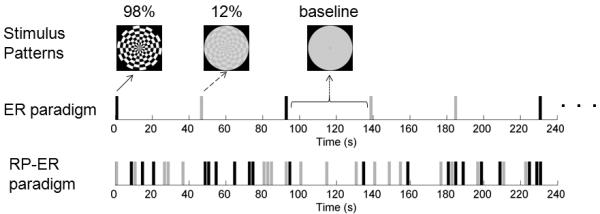
An illustration of the stimuli, the event-related (ER) paradigm, and the rapid presentation (RP) ER paradigm. The black bar represents the 98% contrast stimulus and the gray bar the 12% contrast stimulus.
The ER activation protocol was comprised of five scans, and each scan lasted six minutes and eight seconds. Subjects were presented two visual stimuli consisting of a black-and-white polar checkerboard pattern (circular shape with a diameter of 18.1 degree) with two different Michelson contrasts: 12% and 98% (mean luminance of 110 cd/m2) (Fig. 1, top panel). (The curve of luminance versus stimulus digital value was measured using a luminance meter (Konica Minolta Sensing Americas, Inc., Ramsey, NJ) to find the proper digital values for the Michelson contrast of 12% and the mean luminance.) For each trial, one stimulus was presented for 2 s and contrast reversed at a rate of 10 Hz, followed by 44 s of blank screen with the mean luminance of the stimuli. Each scan had 4 trials for each stimulus presented in a pseudo-random order.
The resting-state fMRI protocol comprised three 184 s long scans for measuring MR signal intensity fluctuations at resting-state without stimulation presentation. The first two scans had the same spatial locations (16 slices) and temporal resolution (TR = 1 s) as the above two protocols: one with eyes-closed and the other with eyes-opened. The subjects were asked to not think anything during the eyes-closed scan. For the eyes-opened scan, the subjects were asked to fixate on a mark at the center of the otherwise blank screen. The third scan had a higher temporal resolution of TR = 250 ms, but with only 4 slices at the same locations as the central 4 slices of the above 16 slices. This high-temporal resolution scan avoided any possible aliasing effects of the cardiac pulsation- and respiration-induced changes to the MR signal. The subjects were also asked to fixate on a mark at the center of the otherwise blank screen during the scan.
Functional imaging session II consisted of the last two protocols in session I plus a RP-ER activation protocol (Fig.1, bottom panel). The RP-ER activation protocol was comprised of three 240 s long scans. The three RP-ER scans were randomly intermixed with the five ER activation scans, and the same two stimuli were used in all these scans. Each stimulus was presented for 1.6 s in both the ER scans and the RP-ER scans. During the RP-ER scans, the minimum inter-stimulus interval was chosen to be 400 ms that minimized both the forward and the backward masking effects (i.e., nonlinear neuronal activities) between any two consecutive stimuli (Macknik and Livingstone, 1998; Huang et al., 2006). In each RP-ER scan, each stimulus was presented 20 times, resulting in a mean inter-trial interval of 6 s. The stimulus presentation pattern was chosen as the one with the maximum efficiency among 100 randomly generated patterns with the constraint of a minimum 2 s stimulus-onset asynchrony (the interval between the onsets of any two stimuli) (Liu and Frank, 2004). For a given stimulus presentation pattern, a 120×33 design matrix (X) was constructed for computing the efficiency of the pattern. The 120 rows in the design matrix represent the 120 time points for each 240 s RP-ER scan (assuming a TR of 2 s instead of 1 s for dramatically improving the computing efficiency). The 33 columns comprised 15 columns of shifted binary stimulus patterns for each stimulus type plus 3 columns that modeled a second order polynomial for the baseline signal (Liu and Frank, 2004). (The hemodynamic response duration was assumed to be 30 s, and the response remained invariant from trial to trial.) The efficiency was computed as the inverse of the sum of the first 30 diagonal terms of the variance-covariance matrix (XT X)−1.
To maintain the subjects’ fixation and attention during all functional scans except the eyes-closed scan, the color of the fixation mark at the center of the visual field randomly changed among red, green, and blue. Time duration between any two consecutive changes varied randomly from change to change, and the mean duration was 3 s for the whole scan. The subjects were instructed to respond to the three colors by pressing three different buttons. The subjects’ responses were recorded and used for off-line analysis. The mean correct response rate in a session ranged from 78% to 95% with mean response times in the range of 710 – 1070 ms.
At the end of each session, T1-weighted whole-brain images were also acquired. These images were used to reconstruct a cortical surface model for retinotopic mapping analysis. For these three subjects who had both session I and session II, these whole-brain images from the two sessions were also used to co-register each other for each subject, respectively.
Image Acquisition
Functional brain images covering the visual cortex were acquired on a GE 3.0 T scanner using a gradient echo Echo-Planar-Imaging pulse sequence. Except the resting-state scan with the 250 ms temporal resolution, all scans had a field of view covering the whole occipital cortex with the following parameters: TE/TR = 27.9/1000 ms, flip angle 60°, in-plane FOV 23×23 cm2, matrix 64×64, slice thickness 4.0 mm, 16 slices in the axial plane. The 250 ms temporal resolution scan was acquired with TE/TR = 27.9/250 ms, flip angle 30°, 4 slices in the axial plane with the same matrix and the slice thickness as above. The 4 slices were chosen at the same locations as the central 4 slices of the 16 slices in the other scans and covered a large part of the calcarine sulcus. The stimulation presentation was controlled by a PC equipped with the Psychophysics Toolbox extension for Matlab (Brainard 1997). The visual stimuli were projected onto a vertical screen placed inside the magnet bore using a custom-made projection system with a 23°×30° visual field angle placed at the back of the magnet room. The projection system was connected to the PC outside the scanner room via an optical fiber. Subjects viewed the stimuli through a mirror attached to the MRI head coil. Image acquisition was synchronized with the stimulus presentation. A BrainLogics Fiber Optic Button Response System with a pair of 5-button MR-compatible keypads (Psychology Software Tools, Inc., Pittsburgh, PA) was used to record subjects’ responses. The respiration and cardiac pulsation signals were recorded using a pneumatic belt placed around the subject’s upper abdomen and a pulse oximeter attached on the subject’s left index finger, respectively, for all subjects except one in session I. For the participants who needed vision correction, MRI-compatible lenses were used. T1-weighted whole-brain MR images were acquired using a 3D inversion-recovery spoiled gradient recalled (IR-SPGR) pulse sequence with a spatial resolution of 0.90×0.90×2.0 mm3.
Image preprocessing
Image preprocessing of the functional images was performed using AFNI (http://afni.nimh.nih.gov/afni), including (1) slice-timing correction of the image acquisition time difference from slice to slice; (2) motion correction of the images to align all volume images from all scans to the very last volume images of 16 slices of the very last functional scan; (3) voxelwise normalization of a signal intensity time course by dividing it with its mean signal intensity value for each scan; and (4) voxelwise temporal drift correction to remove slow linear and second order baseline shifts in the signal intensity time course. After the preprocessing steps, further image analysis was carried out using in-house developed Matlab-based software algorithms.
Retinotopic Mapping
The phases of the periodic activation corresponding to the spatial locations of the rotating wedges and the dilating/contracting rings were obtained by discrete Fourier transformation (DFT) analysis of the signal intensity time courses for the two stimuli in each moving condition (counter-clockwise or clockwise rotating for wedges and contracting or expanding for rings). Considering that it takes one cycle of stimulation to initiate a BOLD response for each spatial location, the periodic BOLD response for all spatial locations starts from the beginning of the second cycle. Accordingly, for each moving condition, the images acquired during the first cycle were excluded from the DFT analysis to avoid this stimulus onset effect. The phase uncertainty due to the time delay of BOLD responses was removed by subtracting the phase during the counter-clockwise rotation of the wedge from that during the clockwise rotation, and it is the same for the expansion and contraction of the rings (Sereno et al., 1995). The retinotopic maps of polar angle and eccentricity were visualized using SUMA (http:/afni.nimh.nih.gov/afni/suma) on the cortical surface. (Each subject’s cortical surface was first reconstructed from the subject’s T1-weighted high-resolution whole brain images using FreeSurfer software (http://surfer.nmr.mgh.harvard.edu/), and then viewed in AFNI via SUMA.) The borders of visual areas were manually drawn, based on phase reversals in the polar angle map, and the visual areas (V1, V2, V3, V3A, and V4) were identified for each hemisphere. These surface visual areas were represented as interconnecting surface nodes in FreeSurfer and were used for constructing the 3D volume masks corresponding to the visual areas. For each surface node in a visual area, a 3 mm line segment perpendicular outward to the surface of the white/gray matter boundary was generated in 3D image space and used to examine voxels for constructing a 3D volume mask. For a given voxel, the intersections of the voxel with all segments from the visual areas were first examined and then the voxel was assigned to the visual area with the most segments intersected by the voxel. Voxels not intersected with any segment were excluded from the 3D volume masks.
Activation analysis
Functional images from the five ER scans were sorted according to the stimulus contrast and then concatenated to form a time course (a total of 920 time points) including all trials for each contrast, respectively. For each contrast, the correlation coefficient (CC) between the concatenated time course and an ideal hemodynamic response function was computed voxel-by-voxel. The ideal response function is a gamma density function f(t)= tδ exp(−t/τ) withδ = 9.0 ,τ = 0.7 , and t in units of second (Boynton et al, 1996). Activated voxels were determined as those with CC>0.11 (p =0.0008 with the 920 time points, no correction for multiple comparisons) for both contrasts. For each activated voxel, a mean signal change time course was obtained by averaging the signal change time courses over all the trials of the same contrast. The peak height of the mean signal change time course was computed as the mean of the three neighboring data points around the peak, and the undershoot depth was computed as the mean of the five neighboring data points around the bottom. All activated voxels within each visual area were included to form a region of interest (ROI) for that area, and a ROI averaged signal change time course was further computed by averaging the mean signal change time courses over all the voxels within the ROI.
To accurately determine the response peak height and the undershoot depth requires an accurate determination of the signal intensity baseline for each trial. However, unexpected large signal changes could occur during the baseline periods for some trials though the sources for the changes may not be known (e.g., sudden head movements, large local physiological changes, etc.). Including these trials would alter the baseline and consequently yield additional errors to the measurements of peak height and undershoot depth. To identify these trials, a mean signal intensity time course over the activated voxels for each trial was first computed and then visually examined. Comparing to the response peak height, a trial showing a comparable size of signal changes during the undershoot and baseline period was excluded from further analysis. As a result, the percentage number of excluded trials was 0%, 0%, 5%, 17.5%, 25%, and 42.5%, respectively, for the six subjects in imaging session I. In imaging session II, the values were 7.5%, 10%, and 25%, respectively, for the three subjects. Our analysis showed that all the main conclusions remained the same with or without excluding these trials, though the variations were smaller for the former than the latter.
Blood volume fraction index
Since MR signal intensity in large vessels is relatively low due to the short transverse relaxation time of blood water and variation is high due to substantially large physiological noise, the ratio of the standard deviation (SD) to the mean of MR signal intensity time courses provides a measure for differentiating voxels containing large vessels from those containing microvasculature (Zhang et al., 2008). A voxelwise blood volume fraction index (υ) was computed for both the ER and resting–state scans. For the ER scans, the SD of the baseline period (the last 7 time points of 40-46 s from the stimulus onset) was computed first for each trial, and then the index υ was computed as the root mean square of the SDs for all trials for each contrast, respectively. For each of the two resting-state scans with the same temporal resolution as that of the ER scans, the index υ was computed as the SD of the normalized signal intensity time course. To compare the BOLD response in voxels containing large vessels with those containing microvasculature, for each subject, the median value (υmedian) of the indices for all activated voxels in each visual area was used for differentiating voxels containing large vessels (υ > υmedian) from those containing microvasculature (υ < υmedian).
Functional images of the resting-state scan with the high-temporal resolution (TR=250ms) were used to test the effects of cardiac pulsation and respiration to the blood volume index. The index was computed in the same way above for the resting-state scans; one with corrections of cardiac pulsation- and respiration-induced changes to the MR signal intensity time courses and one without. The cardiac pulsation- and respiration-induced signal changes were corrected using the 3dretroicor program in AFNI with the individually recorded cardiac pulsation and respiration signals (Glover et al., 2000).
Effects of nonlinear BOLD response in the RP-ER paradigm
In a RP-ER paradigm, the BOLD responses to the stimuli are estimated with the assumption of linear BOLD responses. Furthermore, these responses are also assumed to last for a certain period of time (e.g., 20 s) and to remain invariant from trial to trial. The measured MR signal intensity at each time point is assumed to be the sum of the magnitudes of the BOLD responses to all stimuli at that time point plus the baseline signal intensity and noise, providing a means for estimating the BOLD response to each stimulus. A linear BOLD response should yield an estimated BOLD response which is the same as that obtained from the ER paradigm. Accordingly, the difference between the estimated BOLD response of the RP-ER paradigm and the BOLD response of the ER paradigm signifies the magnitude of the nonlinear effect of the BOLD response in the RP-ER paradigm. In addition, the assumed duration length (e.g., 20 s) for the BOLD response may also affect the estimated BOLD response. In this study we examined these effects using functional images from imaging session II. Functional images from the three RP-ER scans were concatenated to form a time course, and then the voxelwise time course was analyzed with the least-squares fitting method using the 3dREMLfit function in AFNI to yield an estimated BOLD response to each stimulus. Due to the 1 s temporal resolution of the signal intensity time course, a design matrix size of 720×(2n+9) was used in the least-squares fitting, where n represents the hemodynamic response duration length. Three different duration length of 20, 30, and 40 were used for testing the duration effect. (The last 9 columns in the design matrix were used to model a second order polynomial for the baseline signal.) Functional images of the five ER scans in imaging session II were analyzed in the same way as that in imaging session I described above. Activated voxels were defined as those with the estimated BOLD responses significantly different from the baseline (F-test, F(80, 631) > 1.63, uncorrected p < 0.0008 with a 40 s duration length) and also activated in the ER paradigm.
Results
Correlation of undershoot with BOLD response in the ER paradigm
Functional images from the five ER scans in imaging session I were analyzed to yield the BOLD responses to the 12% and 98% stimulus contrasts in each visual area. The upper panel in Fig. 2 shows the mean BOLD responses to the two contrasts in V1, V2, and V3, respectively. For this ER paradigm, the typical BOLD response reached a peak at ~ 7 s after the stimulus onset, independent of the stimulus contrast and the visual area. The BOLD response also showed a clear undershoot in each visual area for both contrasts; it started at ~ 12 s after the stimulus onset and returned to the baseline at about 35 s. The bottom panel in Fig. 1 shows the peak heights of the responses in the visual areas for the two contrasts (left); the corresponding undershoot depths (middle); and the ratios of the undershoot depths and the peak heights (right). The response peak height for the 98% contrast was significantly larger than that for the 12% contrast in each visual area (maximal p = 0.04; two tail, paired t-test), reflecting the larger neuronal activity evoked by the larger contrast (Gö pfert et al., 1999; Hall et al., 2005). The undershoot depth was generally larger at the 98% contrast compared to the 12% contrast. Generally speaking, both response peak height and undershoot depth decreased from V1 to V3 (Fig. 2, bottom panel, left and middle). However, the ratio of the undershoot depth to the peak height remained at a similar level across the visual areas for both contrasts (Fig. 2, bottom panel, right), suggesting a correlation of the undershoot with the positive BOLD response in the ER paradigm that is independent of the visual area and the stimulus contrast. For the 98% contrast, the mean and SD of the ratio was −0.37±0.13, −0.41±0.18, and −0.38±0.19 in V1, V2, and V3, respectively. It was −0.31±0.08, −0.37±0.20, and −0.43±0.28 in V1, V2, and V3, respectively, for the 12% contrast. The mean ratios for the two contrasts showed no significant difference in any of the visual areas (p values ranged from 0.25 to 0.64), suggesting a more homogeneous rather than a heterogeneous BOLD response across the visual areas in the ER paradigm.
Figure 2.

Visual area BOLD response in the ER paradigm. Top panel: mean signal change time course in V1, V2, and V3 in response to the checkerboard stimuli at 98% and 12% contrasts, respectively. The gray vertical bar represents the stimulation period. The error bar denotes the standard error of the mean. Bottom panel: mean response peak heights (left); mean post-stimulus undershoot depths (middle); and the ratios of the undershoot depths and the peak heights in the three visual areas, respectively. (*: maximal p = 0.04.)
We analyzed the correlation of the undershoot with the positive BOLD response in a visual area using all activated voxels within the area. For a representative subject, the top panel in Fig. 3 shows the scatter plots of the undershoot depth versus the peak height in the three visual areas for the 98% contrast, and the middle panel shows the scatter plots for the 12% contrast, respectively. For each subject, the undershoot depth was found to be significantly correlated with the peak height in all visual areas for both contrasts (p<0.004, except for V3 in one subject where p=0.21). For the 98% contrast, the group (n=6) mean and SD of CC were 0.77±0.13, 0.63±0.21, and 0.60±0.28 in V1, V2, and V3, respectively. Correspondingly, these values were 0.47±0.15, 0.44±0.21, and 0.50±0.13 for the 12% contrast, relatively smaller than those for the 98% contrast. These smaller CC values most likely reflected their corresponding smaller values of peak height and undershoot depth since the noise should remain at the same level for both contrasts. In each visual area, the distribution of undershoot versus peak height was fitted with a straight line of y=ax+b, where x was the peak height, y the undershoot depth, a the slope, and b the intercept (Fig. 3, top and middle panels, solid lines). The group mean and SD of the slope were 0.30±0.11, 0.25±0.12, and 0.25±0.14 at the 98% contrast in V1, V2, and V3, respectively. These values were 0.18±0.09, 0.18±0.10, and 0.25±0.16 for the 12% contrast. The group mean and SD of the intercept were 0.14±0.12, 0.17±0.18, and 0.10±0.08 at the 98% contrast in V1, V2, and V3, respectively. These values were 0.14±0.04, 0.17±0.08, and 0.14±0.10 for the 12% contrast. Considering the contrast as one factor and the visual area as another factor, a two-way ANOVA test for the slopes showed no significant difference in the slope across the area (p=0.80) and the contrast (p=0.13) as well as the interaction between them (p=0.45). Similarly, a two-way ANOVA test for the intercepts showed no significant difference in the intercept across the area (p=0.57) and the contrast (p=0.69) as well as the interaction between them (p=0.87). These results further support a more homogeneous rather than a heterogeneous BOLD response across the visual areas in the ER paradigm.
Figure 3.

Correlations of post-stimulus undershoot depth with response peak height of the activated voxels in V1, V2, and V3, respectively, in a representative subject for the 98% contrast (top panel) and the 12% contrast (middle panel) in the ER paradigm. The straight line in each figure represents the least-squares fitting of the corresponding scatter plot. Bottom panel: correlation of response peak heights between the two contrasts in V1, V2, and V3, respectively, for the same subject. (CC: correlation coefficient; *: maximal p=3.5×10⁻⁹; **: maximal p=2.3×10−53.)
We further analyzed the correlation of the BOLD response to the 12% contrast with that to the 98% contrast. For the representative subject, the bottom panel in Fig. 3 shows the scatter plots of the former versus the latter in V1, V2, and V3, respectively. These two responses were strongly correlated with each other in each visual area for all subjects (maximal p=2.3×10⁻⁶). The mean and SD of CC were 0.88±0.11, 0.87±0.16, 0.84±0.15 in V1, V2, and V3, respectively. The solid line in each figure in the bottom panel in Fig. 3 represents the least-squares fitting of the distribution in that figure, and its slope and intercept were computed. The mean and SD of the slope were 0.67±0.23, 0.70±0.26, and 0.66±0.27 in V1, V2, and V3, respectively. These values are very similar and show no significant difference across the visual areas (F-test; p=0.95). The mean and SD of the intercept were 0.08±0.14 (%), 0.11±0.15 (%), and 0.15±0.15 (%) in V1, V2, and V3, respectively, and they do not differ significantly from zero (p>0.06) in all the visual areas. These results further support the homogeneous BOLD response across the visual areas in the ER paradigm, though the response magnitude varied substantially across each visual area. They also suggest that the magnitude of the BOLD response of the 12% contrast was proportional to that of the 98% contrast, implying that the ratio of the two responses was the same across all the activated voxels within each visual area.
Effect of blood volume fraction to BOLD response in the ER paradigm
Despite the homogeneous BOLD response across the visual areas, the magnitude of the BOLD response varied substantially over a wide range as evidenced in Fig. 3. To examine the effect of blood volume fraction on the BOLD response, we analyzed the correlation of the response peak height with the blood volume fraction index. We first tested the correlations of the indices measured under the four different activation conditions: the ER activation for the 12% contrast, the ER activation for the 98% contrast, the resting-state scan with eyes-closed, and the resting-state scan with eyes-opened (details see Blood volume fraction index under Methods and Materials). The index for the 12% contrast was strongly correlated with that for the 98% contrast in each visual area for each subject (maximal p = 1.0×10⁻¹⁷). The group (n=6) mean and SD of the CC were 0.95±0.03, 0.93±0.06, and 0.89±0.11 in V1, V2, and V3, respectively. Figure 4(A) shows a scatter plot in V1 in a representative subject, demonstrating this strong correlation. The solid line on the figure represents the least-squares linear fitting of the distribution. The mean and SD of the slope of the line were 0.97±0.06, 1.06±0.19, and 1.02±0.22 in V1, V2, and V3, respectively. These values are very close to one, and show no significant difference from one in any of the visual areas (p >0.23, t-test). The mean and SD of the intercept were 0.06±0.04, 0.02±0.06, and 0.05±0.11 in V1, V2, and V3, respectively, very close to zero. Accordingly, the index remained at the same level for both contrasts, showing the independence of the index to the contrasts. The index for the eyes-closed resting state condition was also found to be strongly correlated with that for the 98% contrast in the visual areas for all six subjects (maximal p = 1.1×10⁻¹⁷) with CC values of 0.85±0.07, 0.82±0.08, and 0.87±0.03 in V1, V2, and V3, respectively. Figure 4(B) illustrates this strong correlation in V1 in the representative subject. The index for the eyes-opened resting state condition was also strongly correlated with that for the 98% contrast, and the CC values were 0.85±0.09, 0.82±0.10, and 0.86±0.05 in V1, V2, and V3, respectively (data not shown). All the four different activation conditions yielded similar results, showing the independence of the measured index to the activation conditions. Then, the response peak height was found to be positively correlated with the index in each visual area for each contrast and each subject (maximal p=3.5×10⁻⁹), showing that the BOLD response increased with increasing the blood volume fraction. Figure 4(C) illustrates this correlation in V1 in the representative subject. For the 98% contrast, the mean and SD of the CC were 0.65±0.12, 0.66±0.14, and 0.72±0.13 in V1, V2, and V3, respectively. Correspondingly, these values were 0.71±0.10, 0.68±0.14, and 0.72±0.13 for the 12% contrast. The significantly positive correlation of the response peak height with the index shows that the blood volume fraction affects the BOLD response in the ER paradigm - the larger the blood volume fraction, the larger the BOLD response.
Figure 4.

Correlations among blood volume fraction indices under different activation conditions in a representative subject. (A): Correlation of blood volume fraction indices between the two contrasts in V1. The strong correlation shows the independence of the measured index ν to the stimulus contrasts. (B): Correlation of blood volume fraction indices between the eyes-closed resting-state scan and the 98% contrast in V1. The strong correlation shows the independence of the measured index ν to the activation conditions. (C): Correlation of BOLD response peak height with blood volume fraction index at 98% contrast between in V1. The positive correlation shows that the blood volume fraction affects the BOLD response – the larger the blood volume fraction, the larger the magnitude of the BOLD response. The solid line in each figure represents the least-squares fitting of the scatter plot. (CC: correlation coefficient; *: p<8.7×10−36; **: p<2.5×10−78.)
To compare BOLD responses in voxels containing large vessels (υ > υmedian) with those containing microvasculature (υ < υmedian), a mean response was computed in each visual area for each contrast, respectively. Fig. 5 (A) shows the group averaged (n=6) signal change time courses at the 98% contrast in V1 for the large vessel and the microvasculature, respectively. The response for the large vessel was almost twice as that for the microvasculature, consistent with the positive correlation of the response peak height with the index. As expected the undershoot depth for the former was also almost twice as that for the latter, reflecting the strong correlation of the undershoot depth with the response peak height. To further analyze these responses, the signal change time courses were normalized by dividing them with their corresponding peak heights (Fig. 5(B)). The normalized BOLD response for the large vessel was almost identical to that for the microvasculature, though the former was slightly delayed ~ 1 s relative to the latter, further supporting the homogeneous BOLD response in the ER paradigm. Similar behaviors were observed for the BOLD responses in all the visual areas for both contrasts.
Figure 5.

Effects of the blood volume fraction on the BOLD response. (A): Comparison of group (n=6) mean BOLD responses to the 98% contrast in V1 in the ER paradigm for the voxels containing large vessels (ν > νmedian) with those containing microvasculature (ν < νmedian). Both response peak height and undershoot depth for the large vessel were about twice as large as those for the microvasculature. (B): The normalized responses by dividing these responses with their corresponding peak heights. These normalized responses were almost identical to each other, though one was delayed ~ 1 s, providing further evidence to a homogeneous BOLD response in the ER paradigm. The error bars denote the standard errors of the mean.
To test the effects of cardiac pulsation and respiration to the blood volume fraction index, we first computed the index for the high-temporal resolution (TR=250 ms) scan with and without the correction of cardiac pulsation- and respiration-induced changes to the MR signal intensity time course, respectively. Then, we analyzed the correlation of these two indices for the five subjects whose cardiac pulsation and respiration signals were recorded. They were strongly correlated with each other for each subject (maximal p=1.3×10−81), and the group (n=5) mean and SD of the CC were 0.98±0.01. Figure 6(A) illustrates this correlation in a representative subject. The solid line on the figure represents the least-squares linear fitting of the distribution. The mean and SD of the intercept of the line was 0.05±0.06, not significantly different from zero (p=0.168). The mean and SD of the slope, however, was 0.88±0.09, significantly different from one (p = 0.038), showing that the cardiac pulsation and respiration corrections reduced the calculated blood volume fraction index value by 12% compared to that without the corrections. We also analyzed the correlation of the index for the high-temporal resolution scan with that for the low-temporal resolution (TR=1 s) scan (eyes-opened), and found that they were also strongly correlated with each other for each subject (maximal p=9.8×10⁻²⁵). The group (n=5) mean and SD of the CC were 0.88±0.01. Figure 6(B) illustrates this correlation in the representative subject. The mean and SD of the intercept of the line was 0.07±0.07, not significantly different from zero (p=0.10). The mean and SD of the slope was 0.68±0.07, significantly different from one (p = 0.001), showing that the calculated blood volume fraction index value for the low-temporal resolution scan was smaller than that for the high-temporal resolution scan.
Figure 6.

Correlations of blood volume fraction indices for different conditions in a representative subject. (A): Correlation of blood volume fraction indices for the high-temporal resolution (TR=250 ms) scan with and without the corrections to the cardiac pulsation- and respiration-induced changes to the MR signal intensity time course. (B): Correlation of blood volume fraction indices between the low-temporal resolution (TR=1 s) scan (eyes-opened) with the high-temporal scan without the corrections to the cardiac pulsation- and respiration-induced changes to the MR signal intensity time course. The solid line in each figure represents the least-squares linear fitting of the scatter plot. (CP&R: cardiac pulsation and respiration; CC: correlation coefficient; *: p=9.8×10⁻²⁵; **: p=1.3×10−81.)
Effects of nonlinear BOLD response in the RP-ER paradigm
Prior to the analysis of the effect of nonlinear BOLD response in the RP-ER paradigm, we analyzed the BOLD responses to the stimuli in the ER scans from imaging session II for the three subjects. The mean BOLD responses in the three visual areas are plotted in Fig. 7; the black solid lines in top panel for the 98% contrast and bottom panel for the 12% contrast, respectively. These responses are similar to those in the ER paradigm from imaging session I (top panel in Fig. 2), demonstrating the reproducibility and the reliability of these responses in the ER paradigm.
Figure 7.

Comparison of group (n=3) mean BOLD responses to the 98% contrast (top panel) and the 12% contrast (bottom panel) in V1, V2, and V3, respectively, for the ER and RP-ER paradigms. For the RP-ER paradigm, the BOLD response was estimated using a linear BOLD response model with three different duration length of 20 s, 30 s, and 40 s, respectively. The response peak height for the RP-ER paradigm was smaller than that for the ER paradigm, demonstrating a nonlinear BOLD response in the RP-ER paradigm.
For the RP-ER paradigm, the BOLD response to each stimulus was estimated for each subject. The mean estimated responses for all three subjects are plotted in Fig. 7 for comparison with the responses in the ER paradigm. The peak height of this estimated response was smaller than the response peak height in the ER paradigm in each visual area for each stimulus contrast, reflecting a reduction effect of the nonlinear hemodynamic response to the estimated BOLD response in the RP-ER paradigm. Fig. 8(A) shows the reduced mean estimated response peak heights for the RP-ER paradigm compared to the mean response peak heights for the ER paradigm. This reduction effect was also observed in several RP-ER or paired-stimulus ER studies with closely spaced stimuli (Huettel and McCarthy, 2000; Inan et al., 2004; Heckman 2007; Zong and Huang 2010). Although the peak heights of the estimated responses for the RP-ER paradigm were reduced in each visual area for both contrasts, the ratio of the peak height between the RP-ER paradigm and the ER paradigm remained at a very similar level in all the visual areas for both contrasts (Fig. 8(B), left), demonstrating a more homogeneous rather than a heterogeneous reduction effect of the nonlinear hemodynamic response to the estimated BOLD responses in the RP-ER paradigm. The ratio of the peak height between the 12% contrast and the 98% contrast also remained at a similar level in all the visual areas for both paradigms (Fig. 8(B), right), providing further evidence supporting the homogeneous reduction effect of the nonlinear hemodynamic response to the estimated responses in the RP-ER paradigm. Interestingly, in each visual area for each stimulus contrast, the peak height of the estimated response was almost the same for the three different duration length of 20 s, 30 s, and 40 s, though the BOLD response was clearly not returned back to the baseline for the short duration of 20 s (Fig. 7). This result showed that in the RP-ER paradigm the assumed duration length for the BOLD response has a negligible effect on the peak height of the estimated BOLD response as long as the assumed duration length is reasonable (e.g., 20 s).
Figure 8.

Comparisons of the BOLD responses for the ER and RP-ER paradigms. (A): Comparison of BOLD response peak heights in V1, V2, and V3, respectively, for the ER and RP-ER paradigms, demonstrating a reduced response in the RP-ER paradigms in each visual area for each stimulus contrast. (B): Left: Comparison of the ratio of the peak height of the RP-ER paradigm to that of the ER paradigm in V1, V2, and V3, respectively, for the 12% and 98% contrasts; These ratios remained at a similar level across the visual areas, demonstrating a more homogeneous rather than a heterogeneous nonlinear BOLD response in the RP-ER paradigm. Right: Comparison of the ratio of the peak height at 12% contrast to that at 98% contrast in V1, V2, and V3, respectively, for the ER and RP-ER paradigms. These ratios remained at a similar level in each visual area, indicating same relative magnitudes of BOLD responses across stimulus conditions for both the ER and RP-ER paradigms. The error bars denote the standard errors of the mean.
We analyzed the correlation of the peak heights of the estimated responses between the two contrasts using all activated voxels in each visual area. For a representative subject, the top panel in Fig. 9 shows the scatter plots of the peak height of the estimated response at the 12% contrast versus that at the 98% contrast in V1, V2, and V3, respectively. These peak heights were significantly correlated with each other in each visual area for each subject (maximal p=4.2×10⁻¹⁷). The group averaged (n=3) CC were 0.96±0.02, 0.95±0.02, 0.97±0.01 in V1, V2, and V3, respectively, similar as those for the ER paradigm (Fig. 3, bottom panel). Furthermore, the estimated response peak height for the RP-ER paradigm was significantly correlated with the response peak height for the ER paradigm in each visual area for each contrast and each subject (maximal p=8.4×10⁻¹⁶). The bottom panel in Fig. 9 illustrates these correlations for the representative subject. For the 98% contrast, the mean and SD of the CC were 0.94±0.02, 0.88±0.09, and 0.94±0.06 in V1, V2, and V3, respectively. These values were 0.89±0.04, 0.89±0.03, and 0.94±0.02 for the 12% contrast. The black solid line in each figure in the bottom panel in Fig. 9 represents the least-squares linear fitting of the distribution for the 98% contrast. Correspondingly, the red dashed line represents the least-squares linear fitting of the distribution for the 12% contrast. For the 98% contrast, the slope of the fitted line was 0.85±0.07, 0.79±0.03, and 0.83±0.05 in V1, V2, and V3, respectively. These values were 0.67±0.04, 0.68±0.03, and 0.75±0.05 for the 12% contrast. These slope values are less than one, reflecting the reduction effect of the nonlinear hemodynamic response to the estimated BOLD responses in the RP-ER paradigm. The highly significant correlations of the estimated responses of the RP-ER paradigm with the responses of the ER paradigm across the visual areas for both contrasts strongly suggest an approximately homogeneous reduction effect of the nonlinear hemodynamic response to the estimated responses in the RP-ER paradigm.
Figure 9.

Correlations of the response peak heights in each visual area in a representative subject. Top panel: Correlation of response peak heights between the 12% contrast and the 98% contrast in the RP-ER paradigm for activated voxels in V1, V2, and V3, respectively. The strong correlations in the visual areas provide evidence to a homogeneous nonlinear BOLD response in the RP-ER paradigm. The solid line in each figure represents the least-squares fitting of the scatter plot. Bottom panel: Correlation of response peak heights between the two paradigms for activated voxels in V1, V2, and V3, respectively. The black solid and red dashed lines denote the least-squares fittings of the scatter plots at 98% and 12% contrasts, respectively. (CC: correlation coefficient; *: maximal p=6.4×10−39.)
To compare the nonlinear effect in voxels containing large vessels (υ > υmedian) with those containing microvasculature (υ < υmedian), we computed the ratio of the estimated response peak height for the RP-ER paradigm to the response peak height for the ER paradigm in each visual area for each contrast, respectively (Fig. 10). In each visual area for each contrast, the nonlinear effect in the RP-ER paradigm produced a relatively larger reduction in the voxels containing large vessels compared to those containing microvasculature, suggesting a small degree of heterogeneity of the nonlinear hemodynamic response (p=0.12, 0.05, and 0.08 in V1, V2, and V3, respectively, for the 98% contrast, and 0.03, 0.41, and 0.16, respectively, for the 12% contrast).
Figure 10.
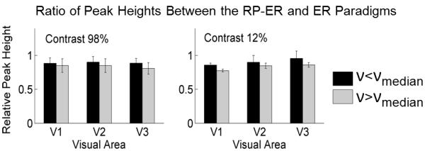
Comparison of the nonlinear BOLD response-induced reduction effect in the RP-ER paradigm in voxels containing large vessels (ν > νmedian) with those containing microvasculature (ν < νmedian). The error bars denote the standard deviations.
Discussion and Conclusions
The similarity of the BOLD signal intensity time course for the two contrasts across the visual areas shows a more homogeneous rather than a heterogonous hemodynamic response in the ER paradigm (Fig. 2, top panel). The strong, voxelwise correlation between the undershoot depth and the BOLD response peak height in each visual area for both contrasts and all subjects provides further evidence to support this conclusion. Although the stimulus-evoked neuronal activity in each visual area was not known, the larger contrast stimulus should evoke a larger neuronal activity in the visual areas as evidenced from EEG and MEG studies (Gö pfert et al., 1999; Hall et al., 2005). Indeed, the amplitude of the BOLD response to the 98% contrast was significantly larger than that to the 12% contrast in each visual area (Fig. 2, bottom panel, left). For a given activated voxel the difference in the neuronal activity was due to the difference between the two contrasts because the stimulus pattern was remained unchanged. This neuronal activity difference might be the same across all the activated voxels within each visual area because the contrast change was uniform across the whole visual field. Within each visual area, the BOLD responses to the two contrasts were strongly correlated with each other, and their distribution followed a straight line with a small intercept that did not differ significantly from zero (Fig. 3, bottom panel). This proportional relationship of the BOLD response between the two contrasts implies a constant ratio between the two responses across all the activated voxels within each visual area. This result suggests that the difference in the underlying neuronal activity between the two contrasts most likely remained a constant across these activated voxels, though a quantitative neuronal activity to each contrast was unknown. It provides a means to link the underlying neuronal activity difference with the BOLD response difference. The large variation in the response peak height for both contrasts showed a large neuronal activity variation across the activated voxels in each visual area, most likely reflecting pattern-evoked different neuronal activity across these activated voxels. Although the BOLD response was affected by the blood volume fraction, the response peak height still varied largely for any given blood volume fraction index (Fig. 4(C)), indicating that the neuronal activity variation from voxel to voxel was mainly responsible for the large BOLD response variation across the visual areas. The larger the neuronal activity, the larger the response peak height as well as the undershoot depth, while the ratio of the latter to the former remained unchanged across the visual areas, reflecting the homogeneous hemodynamic response across the visual cortex in the ER paradigm.
In ER paradigms the neuronal activity is relatively short and induces transient dynamic changes in CBF, CBV, and CMRO2. These transient dynamic changes are tightly coupled together, reflected in the strong correlation between the undershoot depth and the response peak height (Fig. 3, top and middle panels). In contrast, the neuronal activity in block-design paradigms is relatively long, its temporal profile is usually unknown and it may vary spatially across the cortex. Accordingly, the corresponding dynamic changes in CBF, CBV, and CMRO2 may not be tightly coupled, resulting in possibly no relationship or a different relationship between the post-stimulus undershoot and the positive BOLD response. In several block-design studies, the undershoot depth was found to be independent of stimulation intensity (Hoge et al., 1999; Chen and Pike 2009; Sadaghiani et al., 2009). Harshbarger and Song (2008) found a spatial dependence of the post-stimulus undershoots on the vascular and neuronal hierarchy.
The correlation of the peak height with the index υ in Fig. 4(C) provides evidence that the magnitude of the BOLD response is also affected by the blood volume fraction, consistent with the theoretical results of Ogawa et al. (1993) and Obata et al. (2004). The larger the blood volume fraction, the larger the response peak height. This effect also affects the undershoot depth; the larger the blood volume fraction, the larger the undershoot depth. The response peak height varied substantially for a given index υ (Fig. 4(C)), so did the undershoot depth (data not presented). The correlation of the undershoot depth with the response peak height, however, remained unchanged for any given index υ, showing the independence of the correlation to the blood volume fraction. The similarity of the normalized BOLD responses in Fig. 5(B) between the voxels containing large vessels and those containing microvasculature provide further evidence to a homogeneous hemodynamic response across the visual cortex in ER paradigms.
Despite the well-known BOLD nonlinearity, its effect on the estimated BOLD responses in RP-ER paradigms has rarely been investigated (Heckman et al., 2007; Zong and Huang 2010). The source of BOLD nonlinearity could come from either nonlinear neuronal activity and/or nonlinear vascular responses (Birn and Bandettini, 2005; Zhang et al., 2008). Nonlinear neuronal activity would occur when two stimuli are presented too close to each other; the first stimulus would suppress the transient on-response of the second stimulus (forward masking) and the latter would suppress the transient after-discharge of the former (backward masking), resulting in reduced neuronal activity as observed in a cell-recording study (Macknik and Livingstone, 1998) and confirmed in an ER-fMRI study (Huang et al., 2006). This neuronal interaction between the two stimuli diminishes rapidly with increasing the inter-stimulus interval (ISI). In our RP-ER paradigm, the minimal ISI of 400 ms would effectively eliminate the interaction, enabling us to investigate the effect of the nonlinear BOLD response originated from the nonlinear vascular response. The estimated BOLD response in the RP-ER paradigm is smaller relative to the response in the ER paradigm across the visual cortex for both stimulus contrasts (Fig. 7), demonstrating a reduction effect of the nonlinear vascular response in RP-ER paradigms. However, the ratio of the response peak heights of the two contrasts remained approximately the same for the two paradigms (Fig. 8(B), right), suggesting the same scaling effect of the nonlinear vascular response across the stimulus contrasts on the estimated responses in the RP-ER paradigm, consistent with a recent study using a similar RP-ER paradigm (Heckman et al., 2007). Accordingly, in the absence of nonlinear neuronal activity, a scaling to the estimated responses might provide a simple way to account for the nonlinear vascular effect in RP-ER paradigms as noted by Heckman et al. (2007).
The observed nonlinear BOLD effect in our RP-ER paradigm is quite homogeneous across the visual cortex for the two stimulus contrasts. This nonlinear effect is present in both the voxels containing large vessels and those containing microvasculature, and the effect is slightly but not significantly larger in the voxels containing large vessels, further supporting a quite homogeneous nonlinear effect (Fig. 10). In contrast, heterogeneous nonlinear BOLD effects were observed in several studies using different stimulus presentation paradigms (Birn et al., 2001; Pfeuffer et al., 2003; Zhang et al., 2008), suggesting a paradigm-dependent nonlinear BOLD effect. It may reflect different sources responsible for these different nonlinear effects. Birn et al. (2001) observed a significant variation in the nonlinearity across different voxels in the visual and motor cortices in paradigms using stimuli with stimulus durations ranged from 250 ms to 20s, and no correlations were found between the nonlinearity indices and the vascular architecture, suggesting that the nonlinearity might be caused mainly by neuronal nonlinear effects. Pfeuffer et al. (2003) also observed a decreased BOLD impulse response to a visual stimulus with increasing the stimulus duration from 100 ms to 2000 ms, and a spatial dependence of this nonlinear BOLD response across the visual cortex. Using a paired-stimulus paradigm composed of two ultra-short visual stimuli separated by a variable ISI, Zhang et al. (2008) found a decreasing nonlinearity with increasing ISI and a more severe effect in the voxels containing large vessels than those containing microvasculature structures, demonstrating the vascular response as the main source for the nonlinearity since the neuronal responses to all stimuli are identical in the paradigm.
In summary, this study revealed a linear coupling between the positive BOLD response and the post-stimulus undershoot across the visual cortex in an ER paradigm. This voxelwise linear coupling across the visual cortex strongly supports a homogeneous hemodynamic response in ER paradigms. The magnitude of the BOLD response is influenced not only by neuronal activity, but also by the blood volume fraction. The latter effect needs to be accounted for in any quantitative interpretation of the neural event from the BOLD response measurement. In the absence of nonlinear neuronal activities, the nonlinear vascular response renders the estimated BOLD responses smaller in RP-ER paradigms compared to that in ER paradigms, and this reduction effect also needs to be considered for interpreting the estimated BOLD responses in RP-ER paradigms. Interestingly, the reduction effect might be simply modeled by a scaling factor, though the effectiveness of this modeling requires further investigation.
Highlights.
>We found the correlation of the undershoot with the BOLD response in an ER paradigm. >This voxelwise linear coupling supports a homogeneous hemodynamic response. >The blood volume fraction was found to affect the BOLD response. >We also studied the effect of nonlinear vascular response in a rapid ER paradigm. >The effect might be accounted for by a scaling factor across the visual cortex.
ACKNOWLEDGMENTS
This work was supported in part by NIH grant R21NS054202. We appreciate the Department of Radiology at Michigan State University for providing technical support.
Footnotes
Publisher's Disclaimer: This is a PDF file of an unedited manuscript that has been accepted for publication. As a service to our customers we are providing this early version of the manuscript. The manuscript will undergo copyediting, typesetting, and review of the resulting proof before it is published in its final citable form. Please note that during the production process errors may be discovered which could affect the content, and all legal disclaimers that apply to the journal pertain.
References
- Birn RM, Saad ZS, Bandettini PA. Spatial Heterogeneity of the Nonlinear Dynamics in the FMRI BOLD Response. NeuroImage. 2001;14:817–826. doi: 10.1006/nimg.2001.0873. [DOI] [PubMed] [Google Scholar]
- Birn RM, Bandettini PA. The effect of stimulus duty cycle and “off” duration on BOLD response linearity. NeuroImage. 2005;27:70–82. doi: 10.1016/j.neuroimage.2005.03.040. [DOI] [PubMed] [Google Scholar]
- Boynton G, Engel S, Glover G, Heeger D. Linear Systems Analysis of Functional Magnetic Resonance Imaging in Human V1. J. Neuroscience. 1996;16:4207. doi: 10.1523/JNEUROSCI.16-13-04207.1996. [DOI] [PMC free article] [PubMed] [Google Scholar]
- Brainard DH. The Psychophysics Toolbox, Spatial Vision. 1997;10:433–436. [PubMed] [Google Scholar]
- Buxton RB, Wong EC, Frank LR. Dynamics of blood flow and oxygenation changes during brain activation: the balloon model. Magn. Reson. Med. 1998;39:855–864. doi: 10.1002/mrm.1910390602. [DOI] [PubMed] [Google Scholar]
- Chen J, Pike GB. Origins of the BOLD post-stimulus undershoot. NeuroImage. 2009;46:559–568. doi: 10.1016/j.neuroimage.2009.03.015. [DOI] [PubMed] [Google Scholar]
- Chen W, Zhu XH, Kato T, Andersen P, Ugurbil K. Spatial and Temporal Differentiation of fMRI BOLD Response in Primary Visual Cortex of Human Brain during Sustained Visual Simulation. Magn. Reson. Med. 1998;39:520–527. doi: 10.1002/mrm.1910390404. [DOI] [PubMed] [Google Scholar]
- Dale AM, Buckner RL. Selective Averaging of Rapidly Presented Individual Trials Using fMRI. Human Brain Mapping. 1997;5:329–340. doi: 10.1002/(SICI)1097-0193(1997)5:5<329::AID-HBM1>3.0.CO;2-5. [DOI] [PubMed] [Google Scholar]
- Dale AM. Optimal Experimental Design for Event-Related fMRI. Human Brain Mapping. 1999;8:109–114. doi: 10.1002/(SICI)1097-0193(1999)8:2/3<109::AID-HBM7>3.0.CO;2-W. [DOI] [PMC free article] [PubMed] [Google Scholar]
- Devor A, Tian P, Nishimura N, Teng IC, Hillman EMC, Narayanan SN, Ulbert I, Boas DA, Kleinfeld D, Dale AM. Suppressed neuronal activity and concurrent arteriolar vasoconstriction may explain negative blood oxygenation level-dependent signal. J. Neurosci. 2007;27:4452–4459. doi: 10.1523/JNEUROSCI.0134-07.2007. [DOI] [PMC free article] [PubMed] [Google Scholar]
- Donahue MJ, Stevens RD, de Boorder M, Pekar JJ, Hendrikse J, van Zijl PC. Hemodynamic changes after visual stimulation and breath holding provide evidence for an uncoupling of cerebral blood flow and volume from oxygen metabolism. J. Cereb. Blood Flow Metab. 2008;29:176–185. doi: 10.1038/jcbfm.2008.109. [DOI] [PMC free article] [PubMed] [Google Scholar]
- Donahue MJ, Blicher JU, Østergaard L, Feinberg DA, MacIntosh BJ, Miller KL, Gunther M, Jezzard P. Cerebral blood flow, blood volume, and oxygen metabolism dynamics in human visual and motor cortex as measured by whole-brain multi-modal magnetic resonance imaging. J. Cereb. Blood Flow Metab. 2009;29:1856–1866. doi: 10.1038/jcbfm.2009.107. [DOI] [PubMed] [Google Scholar]
- Ernst T, Hennig J. Observation of a fast response in functional MR. Magn. Reson. Med. 1994;32:146–149. doi: 10.1002/mrm.1910320122. [DOI] [PubMed] [Google Scholar]
- Frahm J, Krüger G, Merboldt KD, Kleinschmidt A. Dynamic uncoupling and recoupling of perfusion and oxidative metabolism during focal brain activation in man. Magn. Reson. Med. 1996;35:143–148. doi: 10.1002/mrm.1910350202. [DOI] [PubMed] [Google Scholar]
- Frahm J, Baudewig J, Kallenberg K, Kastrup A, Merboldt KD, Dechentb P. The post-stimulation undershoot in BOLD fMRI of human brain is not caused by elevated cerebral blood volume. NeuroImage. 2008;40:473–481. doi: 10.1016/j.neuroimage.2007.12.005. [DOI] [PubMed] [Google Scholar]
- Friston KJ, Holmes AP, Worsley KJ, Poline J-P, Frith CD, Frackowiak RSJ. Statistical parametric maps in functional imaging: A general linear approach. Human Brain Mapping. 1995;2:189–210. [Google Scholar]
- Friston KJ, Josephs O, Rees G, Turner R. Nonlinear Event-Related Responses in fMRI. Magn. Reson. Med. 1998;39:41–52. doi: 10.1002/mrm.1910390109. [DOI] [PubMed] [Google Scholar]
- Glover GH, Li TQ, Ress D. Image-Based Method for Retrospective Correction of Physiological Motion Effects in fMRI: RETROICOR. Magn. Reson. Med. 2000;44:162–167. doi: 10.1002/1522-2594(200007)44:1<162::aid-mrm23>3.0.co;2-e. [DOI] [PubMed] [Google Scholar]
- Gö pfert E, Müller R, Breuer D, Greenlee MW. Similarities and dissimilarities between pattern VEPs and motion VEPs. Documenta Ophthalmologica. 1999;97:67–79. doi: 10.1023/a:1001888618774. [DOI] [PubMed] [Google Scholar]
- Hall SD, Holliday IE, Hillebrand A, Furlong PL, Singh KD, Barnes GR. Distinct contrast response functions in striate and extra-striate regions of visual cortex revealed with magnetoencephalography (MEG) Clinical Neurophysiology. 2005;116:1716–1722. doi: 10.1016/j.clinph.2005.02.027. [DOI] [PubMed] [Google Scholar]
- Harshbarger TB, Song AW. Differentiating Sensitivity of Post-Stimulus Undershoot under Diffusion Weighting: Implication of Vascular and Neuronal Hierarchy. PLoS ONE. 2008;3(8):e2914. doi: 10.1371/journal.pone.0002914. [DOI] [PMC free article] [PubMed] [Google Scholar]
- Heckman GM, Bouvier SE, Carr VA, Harley EM, Cardinal KS, Engel SA. Nonlinearities in rapid event-related fMRI explained by stimulus scaling. NeuroImage. 2007;34:651–660. doi: 10.1016/j.neuroimage.2006.09.038. [DOI] [PMC free article] [PubMed] [Google Scholar]
- Hoge RD, Atkinson J, Gill B, Crelier GR, Marrett S, Pike GB. Stimulus-Dependent BOLD and Perfusion Dynamics in Human V1. NeuroImage. 1999;9:573–585. doi: 10.1006/nimg.1999.0443. [DOI] [PubMed] [Google Scholar]
- Hu X, Le TH, Ugurbil K. Evaluation of the early response in fMRI in individual subjects using short stimulus duration. Magn. Reson. Med. 1997;37:877–884. doi: 10.1002/mrm.1910370612. [DOI] [PubMed] [Google Scholar]
- Huettel SA, McCarthy G. Evidence for a Refractory Period in the Hemodynamic Response to Visual Stimuli as Measured by MRI. NeuroImage. 2000;11:547–553. doi: 10.1006/nimg.2000.0553. [DOI] [PubMed] [Google Scholar]
- Inan S, Mitchell T, Song A, Bizzell J, Belger A. Hemodynamic correlates of stimulus repetition in the visual and auditory cortices: an fMRI study. NeuroImage. 2004;21:886–893. doi: 10.1016/j.neuroimage.2003.10.029. [DOI] [PubMed] [Google Scholar]
- Jin T, Kim S-G. Cortical layer-dependent dynamic blood oxygenation, cerebral blood flow and cerebral blood volume responses during visual stimulation. NeuroImage. 2008;43:1–9. doi: 10.1016/j.neuroimage.2008.06.029. [DOI] [PMC free article] [PubMed] [Google Scholar]
- Krüger G, Kleinschmidt A, Frahm J. Dynamic MRI sensitized to cerebral blood oxygenation and flow during sustained activation of human visual cortex. Magn. Reson. Med. 1996;35:797–800. doi: 10.1002/mrm.1910350602. [DOI] [PubMed] [Google Scholar]
- Krüger G, Kleinschmidt A, Frahm J. Stimulus dependence of oxygenation-sensitive MRI responses to sustained visual activation. NMR Biomed. 1998;11:75–79. doi: 10.1002/(sici)1099-1492(199804)11:2<75::aid-nbm504>3.0.co;2-7. [DOI] [PubMed] [Google Scholar]
- Liu TT, Frank LR. Efficiency, power, and entropy in event-related fMRI with multiple trial types—Part I: theory. NeuroImage. 2004;21:387–400. doi: 10.1016/j.neuroimage.2003.09.030. [DOI] [PubMed] [Google Scholar]
- Lu H, Golay X, Pekar JJ, van Zijl PCM. Sustained poststimulus elevation in cerebral oxygen utilization after vascular recovery. J. Cereb. Blood Flow Metab. 2004;24:764–770. doi: 10.1097/01.WCB.0000124322.60992.5C. [DOI] [PubMed] [Google Scholar]
- Huang J, Xiang M, Cao Y. Reduction in V1 activation associated with decreased visibility of a visual target. NeuroImage. 2006;31:1693–1699. doi: 10.1016/j.neuroimage.2006.02.020. [DOI] [PubMed] [Google Scholar]
- Liu H-L, Gao J-H. An investigation of the impulse functions for the nonlinear BOLD response in functional MRI. Magnetic Resonance Imaging. 2000;18:931–938. doi: 10.1016/s0730-725x(00)00214-9. [DOI] [PubMed] [Google Scholar]
- Macknik SL, Livingstone MS. Neuronal correlates of visibility and invisibility in the primate visual system. Nature Neuroscience. 1998;1:144–149. doi: 10.1038/393. [DOI] [PubMed] [Google Scholar]
- Mandeville JB, Marota JJA, Ayata C, Moskowitz MA, Weisskoff RM, Rosen BR. MRI measurement of the temporal evolution of relative CMRO2 during rat forepaw stimulation. Magn. Reson. Med. 1999a;42:944–951. doi: 10.1002/(sici)1522-2594(199911)42:5<944::aid-mrm15>3.0.co;2-w. [DOI] [PubMed] [Google Scholar]
- Mandeville JB, Marota JJA, Ayata C, Zaharchuk G, Moskowitz MA, Rosen BR, Weisskoff RM. Evidence for a cerebral postarteriole windkessel with delayed compliance. J. Cereb. Blood Flow Metab. 1999b;19:679–689. doi: 10.1097/00004647-199906000-00012. [DOI] [PubMed] [Google Scholar]
- Menon RS, Ogawa S, Strupp JP, Anderson P, Ugurbil K. BOLD based functional MRI at 4 tesla includes a capillary bed contribution: echo-planer imaging correlates with previous optical imaging using intrinsic signals. Magn. Reson. Med. 1995;33:453–459. doi: 10.1002/mrm.1910330323. [DOI] [PubMed] [Google Scholar]
- Miller KL, Luh W-M, Liu TT, Martinez A, Obata T, Wong EC, Frank LR, Buxton RB. Nonlinear Temporal Dynamics of the Cerebral Blood Flow Response, Human Brain Mapping. 2001;13:1–12. doi: 10.1002/hbm.1020. [DOI] [PMC free article] [PubMed] [Google Scholar]
- Obata T, Liu TT, Miller KL, Luh W-M, Wong EC, Frank LR, Buxton RB. Discrepancies between BOLD and flow dynamics in primary and supplementary motor areas: application of the balloon model to the interpretation of BOLD transients. NeuroImage. 2004;21:144–153. doi: 10.1016/j.neuroimage.2003.08.040. [DOI] [PubMed] [Google Scholar]
- Ogawa S, Menon RS, Tank DW, Kim S-G, Merkle H, Ellermann JM, Ugurbilt K. Functional brain mapping by blood oxygenation level-dependent contrast magnetic resonance imaging: A comparison of signal characteristics with a biophysical model. Biophys. J. 1993;64:803–812. doi: 10.1016/S0006-3495(93)81441-3. [DOI] [PMC free article] [PubMed] [Google Scholar]
- Pfeuffer J, McCullough JC, Van de Moortele P-F, Ugurbil K, Hu X. Spatial dependence of the nonlinear BOLD response at short stimulus duration. NeuroImage. 2003;18:990–1000. doi: 10.1016/s1053-8119(03)00035-1. [DOI] [PubMed] [Google Scholar]
- Poser BA, van Mierlo E, Norris DG. Exploring the Post-Stimulus Undershoot With Spin-Echo fMRI: Implications for Models of neurovascular Response. Human Brain Mapping. 2011;32:141–153. doi: 10.1002/hbm.21003. [DOI] [PMC free article] [PubMed] [Google Scholar]
- Sadaghiani S, Uğurbil K, Uludağ K. Neural activity-induced modulation of BOLD poststimulus undershoot independent of the positive signal. Magnetic Resonance Imaging. 2009;27:1030–1038. doi: 10.1016/j.mri.2009.04.003. [DOI] [PubMed] [Google Scholar]
- Schroeter ML, Kupka T, Mildner T, Uludag K, von Cramon DY. Investigating the post-stimulus undershoot of the BOLD signal – a simultaneous fMRI and fNIRS study. Neuroimage. 2006;30:349–358. doi: 10.1016/j.neuroimage.2005.09.048. [DOI] [PubMed] [Google Scholar]
- Sereno MI, Dale AM, Reppas JB, Kwong KK, Belliveau JW, Brady TJ, Rosen BR, Tootell RB. Borders of multiple visual areas in humans revealed by functional magnetic resonance imaging. Science. 1995;268:889–893. doi: 10.1126/science.7754376. [DOI] [PubMed] [Google Scholar]
- Vazquez AL, Noll DC. Nonlinear Aspects of the BOLD Response in Functional MRI. NeuroImage. 1998;7:108–118. doi: 10.1006/nimg.1997.0316. [DOI] [PubMed] [Google Scholar]
- Wager TD, Vazquez A, Hernandez L, Noll DC. Accounting for nonlinear BOLD effects in fMRI: parameter estimates and a model for prediction in rapid event-related studies. NeuroImage. 2005;25:206–218. doi: 10.1016/j.neuroimage.2004.11.008. [DOI] [PubMed] [Google Scholar]
- Wandell BA, Dumoulin SO, Brewer AA. Visual Field Maps in Human Cortex. Neuron. 2007;56:366. doi: 10.1016/j.neuron.2007.10.012. [DOI] [PubMed] [Google Scholar]
- Yacoub E, Ugurbil K, Harel N. The spatial dependence of the poststimulus undershoot as revealed by high-resolution BOLD- and CBV-weighted fMRI. J. Cereb. Blood Flow Metab. 2006;26:634–644. doi: 10.1038/sj.jcbfm.9600239. [DOI] [PubMed] [Google Scholar]
- Zhao F, Jin T, Wang P, Kim S-G. Improved spatial localization of post-stimulus BOLD undershoot relative to positive BOLD. NeuroImage. 2007;34:1084–1092. doi: 10.1016/j.neuroimage.2006.10.016. [DOI] [PMC free article] [PubMed] [Google Scholar]
- Zhao F, Zhao T, Zhou L, Wu Q, Hu X. BOLD study of stimulation-induced neural activity and resting-state connectivity in medetomidine-sedated rat. NeuroImage. 2008;39:248–260. doi: 10.1016/j.neuroimage.2007.07.063. [DOI] [PMC free article] [PubMed] [Google Scholar]
- Zhang N, Zhu XH, Chen W. Investigating the source of BOLD nonlinearity in human visual cortex in response to paired visual stimuli. NeuroImage. 2008;43:204–212. doi: 10.1016/j.neuroimage.2008.06.033. [DOI] [PMC free article] [PubMed] [Google Scholar]
- Zong X, Huang J. Maximal Accuracy and Precision of HRF Measurements in Rapid-Presentation ER-fMRI Experimental Designs. Proc. Intl. Soc. Mag. Reson. Med. 2010;18:1132. [Google Scholar]