Abstract
In this paper, we investigate the performance of time-of-flight (TOF) PET in improving lesion detectability. We present a theoretical approach to compare lesion detectability of TOF versus non-TOF systems and perform computer simulations to validate the theoretical prediction. A single-ring TOF PET tomograph is simulated using the SimSET software and images are reconstructed in 2D from list-mode data using a maximum a posteriori (MAP) method. We use a channelized Hotelling observer (CHO) to assess the detection performance. Both the receiver operating characteristic (ROC) and localization ROC (LROC) curves are compared for the TOF and non-TOF PET systems. We first studied the SNR gains for TOF PET with different scatter and random fractions, system timing resolutions, and object sizes. We found that the TOF information improves the lesion detectability and the improvement is greater with larger fractions of randoms, better timing resolution, and bigger objects. The scatters by themselves have little impact on the SNR gain after correction. Since the true system timing resolution may not be known precisely in practice, we investigated the effect of mismatched timing kernels and showed that using a mismatched kernel during reconstruction always degrades the detection performance, no matter whether it is narrower or wider than the real value. Using the proposed theoretical framework, we also studied the effect of lumpy backgrounds on the detection performance. Our results indicated that with lumpy backgrounds, the TOF PET still outperforms the non-TOF PET, but the improvement is smaller compared with the uniform background case. More specifically, with the same correlation length, the SNR gain reduces with bigger number of lumpy patches and greater lumpy amplitudes. With the same variance, the SNR gain reaches the minimum when the width of the Gaussian lumps is close to the size of the tumor.
Keywords: TOF PET, ROC, LROC, lesion detection, channelized Hotelling observer, lumpy background
1. Introduction
In recent years, there has been renewed interest in the time-of-flight (TOF) positron emission tomography (PET) with the introduction of fast and efficient scintillator materials such as lutetium oxy-orthosilicate (LSO), lutetium-yttrium oxy-orthosilicate (LYSO), and lanthanum bromide (LaBr3), high-performance photomultiplier tubes (PMT), and better electronics designs [1, 2, 3, 4, 5]. In TOF PET, the time difference between the detection of two coincidence photons is used to reduce the uncertainty of the annihilation positions. With a timing resolution Tr, where Tr denotes the full-width-at-half-maximum (FWHM) value, the localization uncertainty along a line of response (LOR) is reduced from the length of the LOR to Δdr = cTr/2, where c denotes the speed of light. Thus, TOF PET can achieve noise reduction without increasing the number of events (i.e., increasing the dose or imaging time). Early work of Snyder et al. [6] showed that for a uniform cylinder with a diameter D and a back-projection reconstruction algorithm, the SNR gain of TOF PET over non-TOF PET is proportional to . Similar relationship was also derived by Tomitani [7] by comparing an infinite uniform source for TOF PET to a finite source with diameter D for non-TOF PET. More recently, Harrison et al. [8] demonstrated using Monte Carlo simulations that the SNR improves with TOF but the improvement is less than theoretically predicted. Kimdom et al. [9] studied the effect of random and scatter fraction in the variance reduction of TOF PET using a simple scatter model, and they showed that the TOF gain increases with higher fraction of scatters and randoms. Conti [10] theoretically modified the traditional estimate for the SNR gain by incorporating the random fraction. Karp et al. [5] and Lois et al. [11] showed using both phantom and clinical measurements that TOF PET provides improved contrast recovery versus noise trade-off as well as faster convergence of contrast recovery in hot lesions. Vunckx et al. [15] used an analytic Fisher information based approach to evaluate the image variance of the TOF PET and showed that less benefit of TOF was seen in eccentric and hot regions.
In this paper, we present a theoretical approach to evaluate the performance of TOF PET in lesion detectability. We assess the detection performance by using a channelized Hotelling observer (CHO) and present a theoretical expression of the SNR of the CHO. Computer simulations were performed to validate the theoretical predictions. We used the Monte Carlo simulation package SimSET (Simulation System for Emission Tomography) to model a single-ring TOF PET tomograph [12], and images were reconstructed in 2D using a list-mode maximum a posteriori (MAP) method. Both the receiver operating characteristic (ROC) and localization ROC (LROC) curves were compared for the TOF and non-TOF cases. We first considered detection of a known lesion in a uniform background and studied the SNR gains for TOF PET with different scatter and random fractions, system timing resolutions, object sizes, and tumor sizes. We also studied the effect of mismatched timing kernels, since the real system timing resolution may not be known precisely. In the end, we investigated the effect of lumpy backgrounds on the SNR gains using the theoretical framework alone.
In [13], Surti and Karp reported their experimental evaluation of a simple lesion detection task with a Philips Gemini TF PET/CT scanner using a non-prewhitening matched filter and a list-mode OSEM reconstruction method. In [14], LROC studies were performed on a prototype TOF PET/CT scanner (Siemens Medical Solutions) to detect focal warm lesions. A channelized non-prewhitened observer was used and images were reconstructed using OSEM. Comparing with their work, our work focuses on the theoretical framework for evaluating the lesion detection performance for TOF PET. In addition, we use Monte Carlo simulations to quantify the effects of randoms and scatters on the TOF detectability improvement.
This paper is organized as follows. In Section 2, we describe the system model and the Bayesian framework we used for image reconstruction. In Section 3, we present methods for lesion detection using the CHO and the theoretical expression of the SNR of CHO. Computer simulations and results are given in Section 4 to study the advantage of TOF in lesion detection. Conclusions are drawn in Section 5.
2. System Model and Image Reconstruction
PET data are modelled as a set of independent Poisson random variables where the expectation of the measurements, ȳ ∈ ℛM×1, relates to the unknown tracer distribution x ∈ ℛN×1 through an affine transformation
| (1) |
where y ∈ ℛM×1 is the measured sinogram data, P ∈ ℛM×N the system matrix with the (i, j)th element representing the probability of detecting an event from the jth voxel at the ith line of response (LOR), and r ∈ ℛM×1 the expectation of the background data (scatters and randoms). In this work, the elements in P incorporate the effect of object attenuation, crystal penetration, and scanner geometry (solid angle formulation). They are computed using the multiray-tracing technique that was proposed in [16], and for each TOF LOR modified by a Gaussian TOF kernel
| (2) |
where Δt− and Δt+ denote the lower and upper limits of the time difference of the TOF LOR, with Δdr being the FWHM value of the localization uncertainty, and s is the distance of a voxel from the center of the LOR.
We reconstruct images using a Bayesian approach which regularizes the image through the use of a prior distribution p(x) on the unknown image. We consider a Gibbs prior of the form
| (3) |
where
| (4) |
is the prior energy function, β the regularization parameter controlling the resolution of the reconstructed image, and Z a normalization constant. Nj represents the set of neighborhood of voxel j, klj the inverse of the Euclidean distance between voxel l and j, and V a pair-wise potential function. For quadratic priors, we have
| (5) |
and ϕ can be expressed as with R being a positive semi-definite matrix and ‘′’ denoting vector (or matrix) transpose. Combining the likelihood function and the image prior, the maximum a posteriori (MAP) estimate is given by
| (6) |
| (7) |
where
| (8) |
is the log-likelihood function.
3. Detection Performance Analysis
In this section, we first describe the channelized Hotelling observer (CHO) and then the theoretical expressions of the SNR for the CHO under the MAP reconstruction framework.
3.1. Channelized Hotelling Observer and Observer Performance
For a given reconstructed image x̂, a linear numerical observer computes a test statistic η(x̂) by
| (9) |
where t ∈ ℛN×1 is the observer template. In this work, we use the channelized Hotelling observer (CHO) which has been shown to have a good correlation with human performances [17]. The test statistic of the CHO is
| (10) |
where z = E[x̂|H1]−E[x̂|H0] represents the expected profile of the reconstructed lesion with H0 being the null hypothesis representing lesion absent and H1 the alternative hypothesis representing lesion present. The term U ∈ ℛL×N denotes frequency-selective channels that mimic the human visual system, L the number of channels, n ∈ ℛL×1 the internal channel noise that models the uncertainty in the human detection process, and Σ ∈ ℛL×L the covariance of the channel outputs. If we assume that n is zero-mean Gaussian with a covariance matrix ΣN ∈ ℛL×L, Σ can be expressed as
| (11) |
where Σx̂|H1 ∈ ℛN×N and Σx̂|H0 ∈ ℛN×N denote the covariance matrices of x̂ under H1 and H0, respectively. Here we assumed equal probability for the signal to be present or absent. We used the differences of four Gaussian (DOG) functions with standard deviations σ = 2.653, 1.592, 0.995, 0.573 as our channel function (corresponding to an L = 3) [18]. The SNR of the CHO is given as
| (12) |
Observers (human or numerical) make a decision by comparing the test statistic η with a preset threshold γ0. If η > γ0, we refer to it as a positive decision. A plot of the true positive (TP) rate versus the false positive (FP) rate as γ0 varies is called an ROC curve. One figure of merit for the detection performance is the area under the curve (AUC). When η(x̂) is normally distributed, the AUC is related to the SNR by
| (13) |
where is the error function.
The ROC curve measures the ability of the observer to differentiate whether an image contains a target (e.g., lesion). In order to take into account whether the observer identifies the location of the actual lesion, a localization ROC (LROC) study should be performed. The LROC curve measures the joint ability to detect and correctly localize the lesion in the images. It is a plot of the TP rate with correct localization against the FP rate [25]. Similar with ROC, the AUC value can be used as a figure of merit for LROC.
3.2. Lesion Detectability in MAP Reconstruction
Even though the size of Σ is manageable for the CHO, evaluating equation (12) involves image reconstruction for a large number of data sets, which is time consuming and may not be practically feasible. In the following, we show a theoretical expression of the detection SNR, which can be computed directly without resorting to reconstructed images.
Consider small lesion and low noise situations, we can apply the first-order Taylor series expansion to the MAP estimation x̂(y) around the point y̿ = PE[x] + r and obtain [19, 20]
| (14) |
| (15) |
where F = P′diag[1/ȳi]P is the Fisher information matrix (F ∈ ℛN×N) with P′ representing the backprojection kernel and P the forward projection kernel, x̄1 = E[x|H1] − E[x|H0] the expected lesion profile, and Σx|Hk ∈ ℛN×N the covariance of the image under Hk (k = 0, 1). Direct computation of equation (14) and (15) is time consuming due to the inversion of a large matrix F + βR. Following previous work [20, 21, 22, 23], we approximate F and R as locally stationary, i.e., if we view the jth column of F (and R) as an image associated with the jth voxel, the intensity of the image concentrates in a local region and varies slowly as we move between the columns associated with neighboring voxels. Then equation (14) and (15) can be computed “locally” using a fast Fourier transform (FFT). Consider voxel j1 where the lesion exists, equation (12) can be approximated as
| (16) |
where B ∈ ℛL×L is defined as
| (17) |
| (18) |
and w ∈ ℛL×1 is a column vector with its lth element defined as
| (19) |
{λj, j = 1,…,N} and {μj, j = 1,…,N} are the Fourier coefficients of fj1 and rj1, respectively, with
| (20) |
| (21) |
representing the column vector corresponding to the lesion location of F and R, respectively. ej denotes a unit vector with 1 on its jth element and 0 otherwise, {ξj, j = 1,…,N} the Fourier transform of x̄1, and Ũ = UQ′ the Fourier coefficients of the channel functions. Q and Q′ represent the Kronecker form of the Fourier transform and its inverse, respectively [24]. More details on the computation of λj and μj can be found in [20].
Equation (16) allows fast evaluation of lesion detectability under various conditions because no image reconstruction is involved. We define the TOF SNR gain in lesion detectability as
| (22) |
The theoretical expression shows that the TOF SNR gain depends on the Fisher information matrix F, prior parameters (β and μj), and channel noise. When β = 0, ΣN = 0, and Σx = 0, the TOF SNR gain for detecting a lesion at the center of a large object is about proportional to the object size because the Poisson noise in non-TOF data increases as the object size increases, while the noise in TOF data that affect the point of interest remains unchanged. However, the linear relationship is no longer valid when we consider object variation and/or observer internal noise.
3.2.1. Effect of a Mismatched Timing Kernel
In TOF reconstruction, the system timing resolution is usually assumed to be known accurately in advance and is modeled in the system matrix. However, this is hardly true in reality. While the timing resolution of the current TOF PET systems is fairly stable, it has been shown that it can change significantly with count rate [4]. Therefore, it would be of practical interest to study the effect of using a mismatched timing kernels during reconstruction when the real system resolution is not known precisely. The theoretical SNR for mismatched timing kernels can be easily derived by examining equations (14) and (15). With a mismatched timing kernel, these two equations become
| (23) |
| (24) |
where Fmis = P′diag[1/ȳi]Ptrue and F = P′diag[1/ȳi]P with P being the system matrix used in reconstruction and Ptrue the true system matrix in data generation. Note that the first term in equation (24) is caused by Poisson noise in PET data and thus is independent of Ptrue once ȳ is given. The corresponding CHO SNR is
| (25) |
where Bmis is given by
| (26) |
and wmis is a column vector with its lth element defined as
| (27) |
{λmis,j, j = 1,…,N} are the Fourier coefficients of the column vector corresponding to the lesion location of Fmis.
4. Computer Simulations
In this section, we present computer simulation results to evaluate the detection performance of TOF and non-TOF PET systems under different conditions. We first consider a lesion in a uniform background and perform Monte Carlo simulations to validate the theoretical prediction. We considered the effects of scatter and random fractions, system timing resolutions, object sizes, and mismatched timing kernels. We then use the theoretical framework to study the effects of tumor sizes and lumpy backgrounds on the TOF SNR gains.
We used SimSET to model a single-ring TOF PET tomograph that is similar to what is under development at Lawrence Berkeley National Laboratory. The detector ring has a diameter of 79.5 cm. It consists of 384 crystals of 6.1 mm in width and 25 mm in radial length. The axial dimension of the crystal is set to 10 cm to obtain reasonable sensitivity and scatter fraction, although the axial dimension of the crystal on the prototype system is actually 6.1 mm. The coincidence window was selected as 3 ns and the energy resolution was chosen to be 15%. We set the timing resolution at 200 ps, which corresponds to a FWHM of 30 mm. The time difference of each coincidence pair was first blurred using the Gaussian timing kernel and then discretized into 127 timing bins with a width of 50 ps (7.5 mm).
4.1. Validation using Monte Carlo Simulations
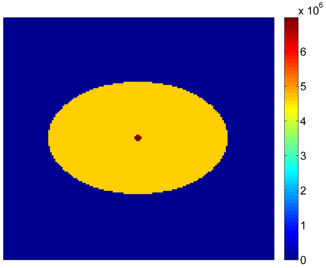
We used a 10 cm long elliptical cylinder with uniform activities as the background (Figure 1). The ellipse has a long axis of 30 cm and a short axis of 20 cm. A hot rod of 12 mm in diameter was placed at the center of the phantom as a lesion. The lesion-to-background activity ratio is 3:2. The true and scatter coincidences were generated by SimSET directly with an energy window between 400 keV and 600 keV. For random coincidences, we first calculated their expectations from the singles rate that was obtained by running the SimSET in SPECT mode, and then we generated each random coincidence as a Poisson realization. Each random coincidence was assigned a time difference that is uniformly distributed among the 127 time bins. We set the initial activity at 100 MBq and obtained an average of 1.06 M prompts in each data set. Each data set took around 1 hour to generate and a total of 200 Monte Carlo simulations were performed. The mean of scatters was computed from these 200 samples. The random fraction (RF = R/(T + S + R)) is around 24.5% and the scatter fraction (SF = S/(T + S)) is around 27.8%. All images were reconstructed from list-mode data using the MAP algorithm with 248×248 3×3×100 mm3 voxels. Scatter and random events were corrected by including the estimated mean scatter and random sinogram in the forward model (1). For the CHO, we selected ΣN = 109I3, where In denotes an identify matrix of dimension n.
Figure 1.
Illustration of the 20 cm × 30 cm phantom used in the simulation. The lesion at the center is 12 mm in diameter with a 3:2 contrast.
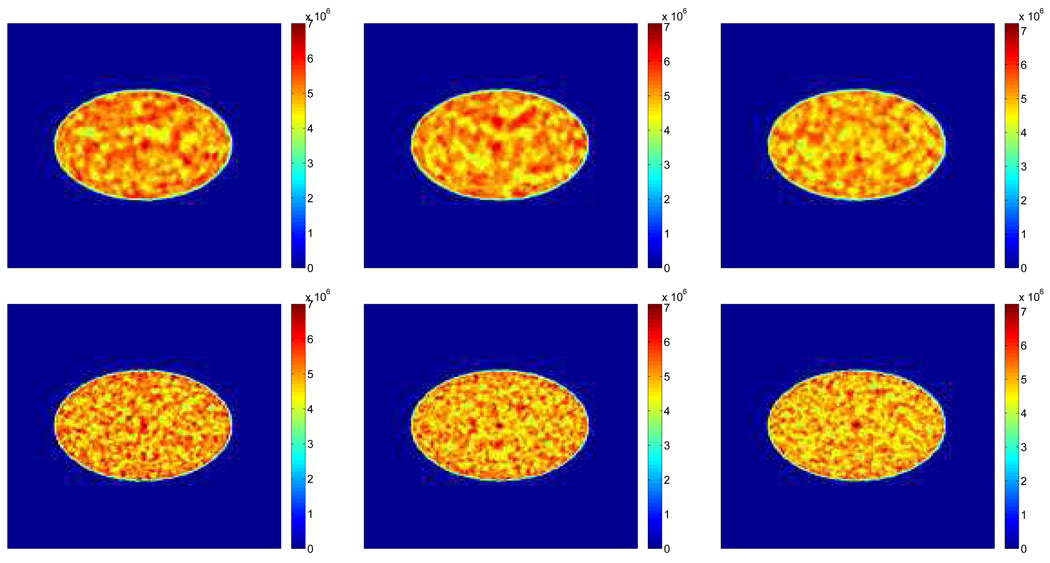
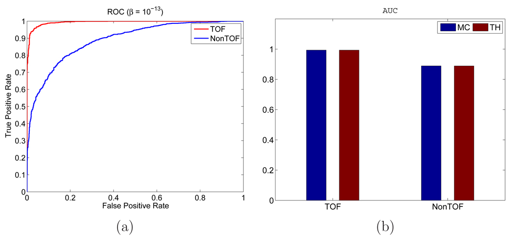
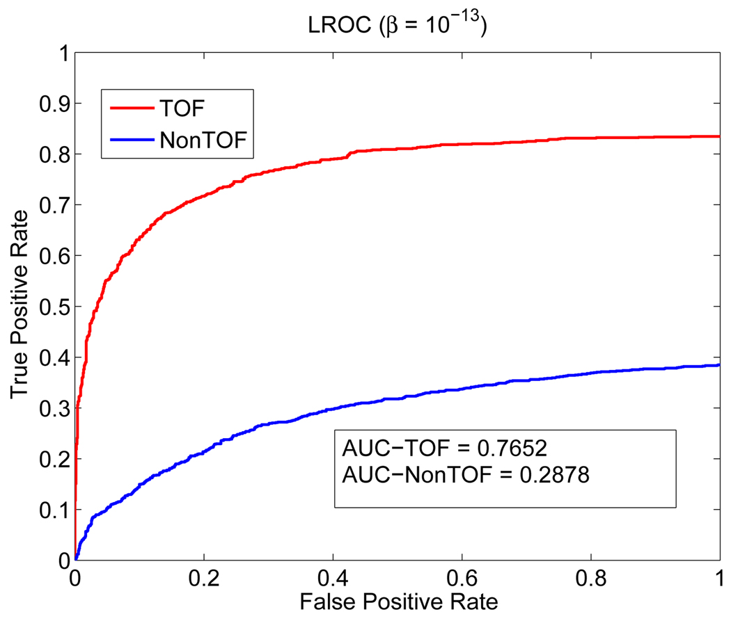
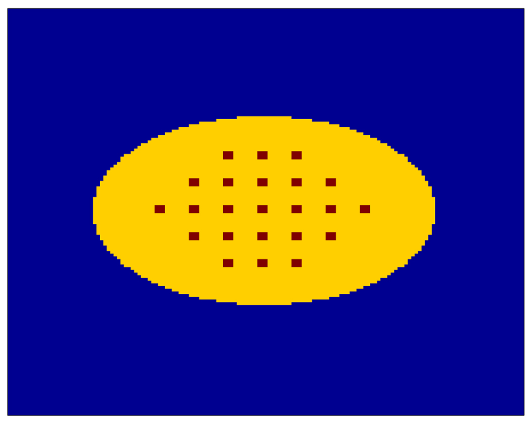
Figure 2 shows examples of reconstructed images from different realizations with and without TOF information. Visually, the lesion is more obvious in the TOF images than the non-TOF ones. To see the effect of β, Figure 3 shows a set of reconstructed images with the lesion present for the TOF PET with β ranging from 10−12 to 10−14. We can see that the image is over-smoothed for β = 10−12 and is very noisy for β = 10−14. In Figure 4(a), we give the ROC curves for the TOF and non-TOF at β = 10−13 and in Figure 4(b), we show the AUC values computed both theoretically (from equation (13) with SNR computed from equation (16)) and from simulation (by numerical integration of the ROC curves). For the current signal-known-exactly and background-known-exactly (SKE-BKE) case (Σx = 0), the ROC curves were obtained by applying the CHO to the reconstructed images and thresholding the resulting test statistics. We can see that the TOF PET (AUCMC = 0.9957) clearly outperforms the non-TOF PET (AUCMC = 0.8894) in terms of lesion detection, and the AUC values computed from Monte Carlo reconstructions match well with the theoretical predictions. In Figure 6, we show the LROC curves for the TOF PET and non-TOF PET at β = 10−13. In this work, we selected 23 non-overlapping areas in the object (see Figure 5) and applied the CHO to each area. The numerical observer is unaware of the correct lesion location and identifies the lesion position by choosing the area with the largest test statistics. The test statistics (equation 10) was modified to consider the channel covariance of each area. We can see that the advantage of the TOF PET is more obvious when the localization ability is considered: the TOF PET has an area of 0.7652 under the LROC curve, whereas the non-TOF PET only has 0.2878. The probability of correctly localizing the lesion with the TOF PET is 80%, whereas with the non-TOF PET it is less than 40% in this study.
Figure 2.
Examples of reconstructed images with β = 10−13. The top row is for the non-TOF reconstruction and the bottom row is for the TOF case. Each column corresponds to a different realization.
Figure 3.
Examples of reconstructed images for TOF PET with different β. (a) β = 10−12. (b) β = 10−13. (c) β = 10−14.
Figure 4.
(a) ROC curves for the TOF PET and non-TOF PET with β = 10−13. (b) AUC values computed from theoretical predictions (in red) and numerical integrations (in blue).
Figure 6.
LROC curves for the TOF PET and non-TOF PET with β = 10−13.
Figure 5.
The selected regions for computing the LROC curve.
4.1.1. Effect of the Random and Scatter Fractions
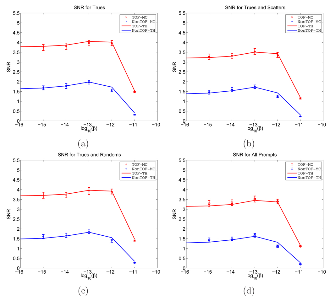
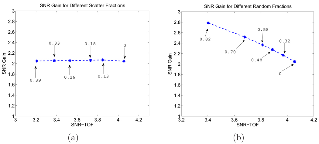
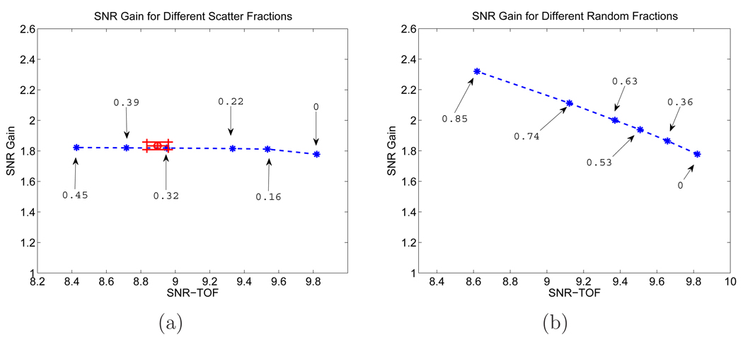
One advantage of using computer simulations is that we can separate true, scattered, and random events, and study their effects on the TOF gain separately. In Figure 7, we show the SNRs computed from theoretical predictions and from Monte Carlo reconstructed images. We considered four different conditions: true events only (579K), true plus scattered events (801K), true plus random events (838K), and all prompts (1.06M). We can see that the SNRs for both TOF and non-TOF are a function of the regularization parameter β, and the values from the Monte Carlo simulation match well with theoretical predications for all four cases. To take a further look at the separate effects of randoms and scatters, in Figure 8, we plot the theoretically predicted SNR gains as a function of the TOF SNR for different random and scatter fractions. The different random fractions were achieved by keeping the trues unchanged and applying a scaling factor to the random distribution. The different scatter fraction was simulated by varying the axial length of the scanner from 4 cm to 25 cm. The sinogram (trues+scatters) for each case was scaled so that they all have the same number of trues. We can see that the SNR gain increases with larger random fraction, but an increase in scatter fraction has little effect on the SNR gain, although it reduces the absolute SNR.
Figure 7.
SNRs computed from theoretical predictions and Monte Carlo reconstructed images under four conditions. (a) True events only. (b) True plus scattered events. (c) True plus random events. (d) All prompts. The solid line represents the SNRs computed from theoretical predictions and the cross indicates the SNRs computed from Monte Carlo reconstructed images. The error bars were obtained from 200 bootstrap samples.
Figure 8.
SNR gains from the theoretical prediction for different (a) scatter and (b) random fractions (β = 10−13). Each point corresponds to a different scatter or random fraction with the corresponding value marked in the plots.
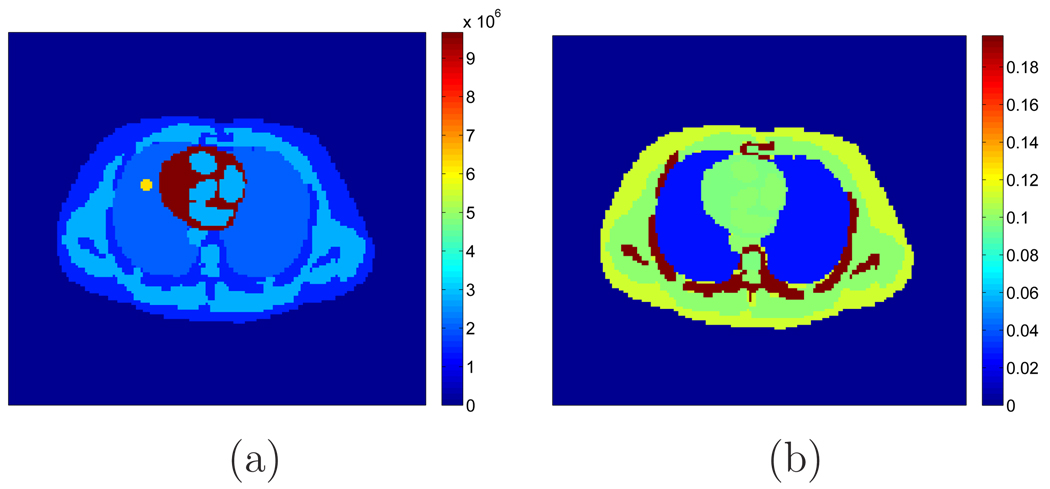
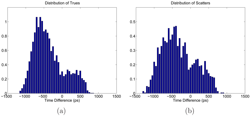
The relative insensitivity of the SNR gain with respect to the scatter fraction is surprising, as scatters were sometimes modeled as events originated from a heavily smoothed object [9]. To verify that this phenomenon is not unique to the uniform phantom, we performed an addition Monte Carlo simulation using an anthropomorphic phantom shown in Figure 9 [26]. The phantom has an activity distribution of myocardium:muscle:blood pool:lung:bone:skin = 14:4:4:3:2:2, and the attenuation coefficient of each organ is provided in Table 1 [12]. A 12-mm diameter lesion was inserted in the left lung and it has a contrast ratio of 3:1 to the lung. Different scatter and random fractions were simulated in the same way as in the uniform phantom simulation. The theoretically computed SNR gain for different scatter and random fractions is shown in Figure 10. To validate our theoretical calculation, we also computed the TOF SNR and SNR gain from 200 Monte Carlo reconstructed images for the scatter fraction of 32% (shown in Figure 10(a) as the red circle with errorbars obtained from 200 bootstrap samples.) We can see that similar to the uniform phantom case, the SNR gain remains relatively insensitive to the scatter fractions and increases as the random fraction becomes larger. This insensitivity of the SNR gain with respect to the scatters is likely due to the fact that scatter events have a similar distribution in time difference as true events. To illustrate this point, we plot in Figure 11 the mean distribution of trues and scatters in the central vertical LOR as a function of time difference. We can see that the trues and scatters share similar distributions in time difference, and the ranges of the time difference are similar as well. Thus the TOF information is not effective in discriminating between trues and scatters.
Figure 9.
(a) A thorax phantom derived from the Zubal phantom. (b) Attenuation map of the thorax phantom (in cm−1).
Table 1.
Attenuation coefficients of the Zubal Phantom (in cm−1)
| myocardium | muscle | blood | lung | bone | skin | |
|---|---|---|---|---|---|---|
| Atn. coef. | 0.098 | 0.099 | 0.1 | 0.025 | 0.197 | 0.113 |
Figure 10.
SNR gains from the theoretical prediction for different (a) scatter and (b) random fractions (β = 10−13) for the Zubal thorax phantom. Each star point corresponds to a different scatter or random fraction with the corresponding value marked in the plots. The red circle in (a) corresponds to the TOF SNR and SNR gain computed from 200 Monte Carlo reconstructed images for the scatter fraction of 32%. The horizontal and vertical error bars are for the TOF SNR and SNR gain, respectively, obtained from 200 bootstrap samples.
Figure 11.
Distribution of the mean of (a) trues and (b) scatters as a function of the time difference for the central vertical LOR.
4.1.2. Effect of the System Timing Resolution
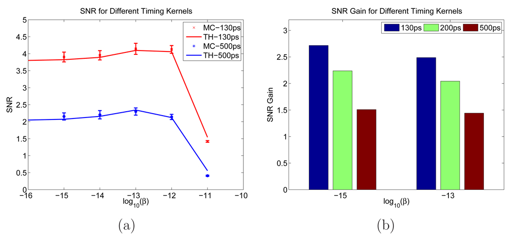
We studied the effect of the system timing resolution on the SNR gain. In addition to the 200 ps timing resolution, we also simulated timing resolutions of 130 ps and 500 ps and reconstructed images using the corresponding values. Examples of reconstructed images are shown in Figure 12. We can see that as the timing resolution gets worse, the lesion becomes less discernible from the background. In Figure 13, we plot the SNR and SNR gains for different system timing resolutions. As we can see, the SNR values increase with better timing resolution and the Monte Carlo simulation results match well with the theoretical predictions. The ratio of the SNR gain between two different systems is proportional to the ratio of the square root of the corresponding system timing resolutions.
Figure 12.
Examples of reconstructed images with different system timing resolutions at β = 10−13. (a) 130 ps. (b) 200 ps. (c) 500 ps.
Figure 13.
(a) SNRs computed from theoretical predictions and Monte Carlo reconstructed images for 130 ps and 500 ps timing resolutions. (b) Monte Carlo simulation based SNR gains for different timing resolutions.
4.1.3. Effect of the Object Size
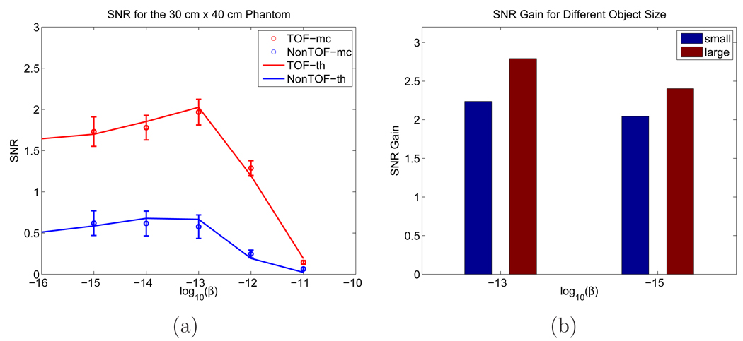
We considered a larger elliptical phantom to study the effect of object size on the TOF SNR gains. The large ellipse has a long axis of 40 cm and a short axis of 30 cm (Figure 14(a)). The lesion size and the activity-background ratio remain the same as in the previous examples. We obtained 100 data sets using SimSET with 1.75 M counts in each realization. The scatter fraction was around 33% and the random fraction was around 48.6%. Examples of reconstructed images using TOF PET and non-TOF PET are shown in Figure 14(b) and Figure 14(c).
Figure 14.
(a) The large phantom (30 cm × 40 cm) used in the simulation. (b) A sample reconstruction of TOF PET data. (c) A sample reconstruction of non-TOF PET data.
The theoretically computed and Monte Carlo simulation based SNR values are given in Figure 15(a) and the corresponding SNR gains are plotted in Figure 15(b) with a comparison with the smaller phantom. We can see that as the patient size becomes larger, the SNR values decreases for both TOF and non-TOF cases. However, the SNR gain is greater for the bigger object and the ratio of the increase is roughly proportional to the square root of the patient size.
Figure 15.
(a) SNRs computed from theoretical predictions and Monte Carlo reconstructed images for the 30 × 40 cm2 phantom. (b) SNR gains from Monte Carlo simulations for objects of different sizes.
4.1.4. Effect of Mismatched Timing Kernels
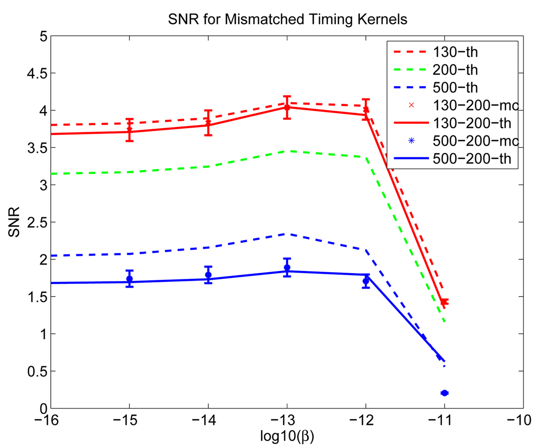
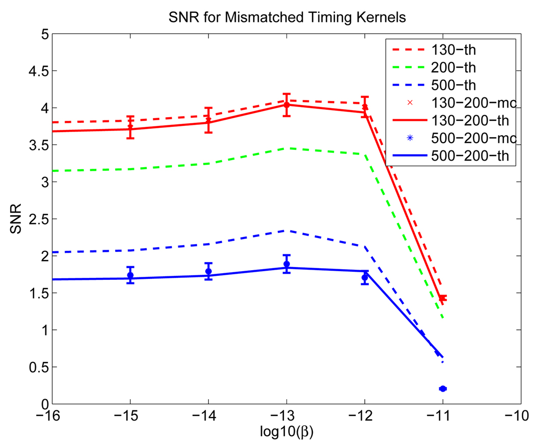
We used the phantom in Figure 1. We generated simulation data with system timing resolution of 130 ps and 500 ps, respectively, and reconstructed all the data using a 200 ps timing kernel. Large mismatch values were used for easier demonstration of the effect. Two hundred data samples were generated for each case. The SNRs from theoretical predictions and Monte Carlo simulations are shown in Figure 16. We can see that the detection performance worsens for both mismatched cases (either using a wider kernel or a narrower one). In general, the performance improves with better timing resolution, but the improvement deteriorates compared with the matched case.
Figure 16.
SNRs computed from theoretical predictions and Monte Carlo reconstructed images for mismatched compared to matched timing kernels.
In Figure 17, we show the theoretically computed SNR when the real system timing resolution is 20% off the reconstructed kernel. More specifically, we assumed that the real timing resolution is 160 ps and 240 ps, respectively, and reconstructed the image using the 200 ps resolution. We can see that compared with Figure 16, the performance degradation is reduced as the mismatch gets smaller. The detection SNR is hardly affected for the 160 ps system when a 200 ps timing resolution is assumed during the reconstruction. The degradation is slightly noticeable when the system resolution is 240 ps and a 200 ps timing kernel is used in reconstruction.
Figure 17.
SNRs computed from theoretical predictions for mismatched compared to matched timing kernels.
4.2. Performance Analysis using the Theoretical Formulae
From Sections 4.1.1–4.1.4, we have shown that the SNR values from Monte Carlo simulations match well with the theoretical predictions. As the theoretical approach does not require any image reconstruction, it can be used as a general framework to study the detection performance under different scenario. In this section, we investigate the effects of the lesion size and lumpy backgrounds on the detection performance.
4.2.1. Effect of the Lesion Size
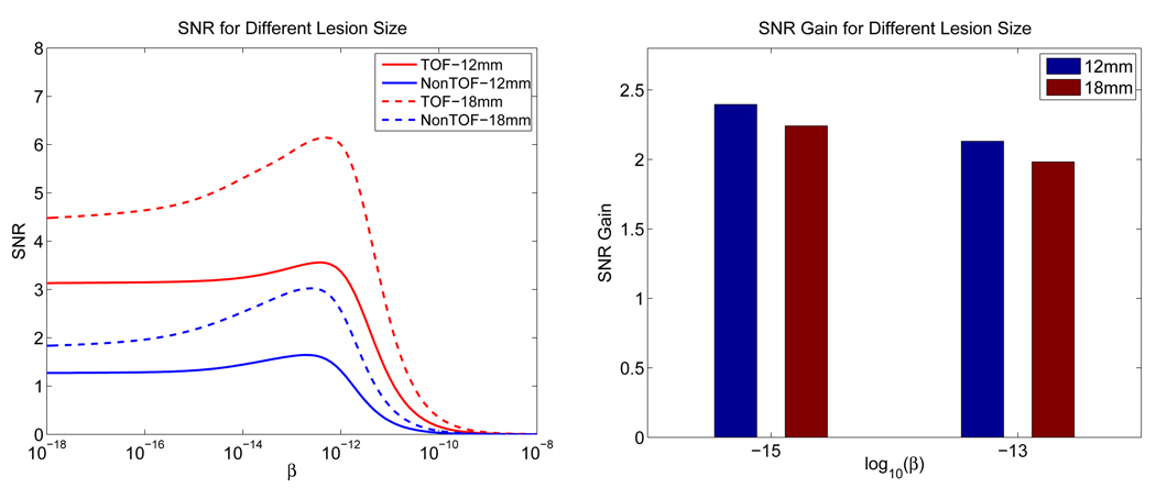
In Figure 18, we show the theoretically computed SNRs for a 12 mm lesion and a 18 mm one, with all the other factors remaining the same. We can see that as the lesion increases in size, the SNR values increase, but the SNR gains for the TOF PET over non-TOF PET actually decreases. The result shows that with other factors being the same, it is less advantageous to use the TOF information for detecting a larger lesion.
Figure 18.
(a) SNRs computed from theoretical predictions for a 18 mm lesion and a 12 mm lesion. (b) Theoretically predicted SNR gains.
4.2.2. Effect of Lumpy Backgrounds
The lumpy background was simulated by randomly superimposing Gaussian functions on a constant background over the phantom space [27]. The lumpy component can be mathematically modeled as
| (28) |
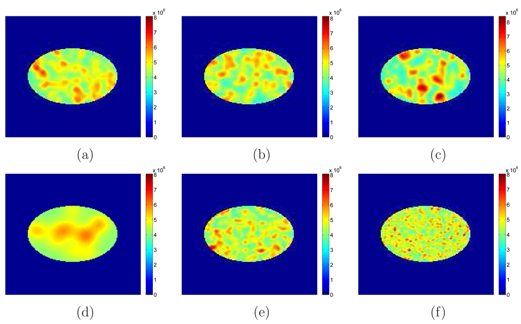
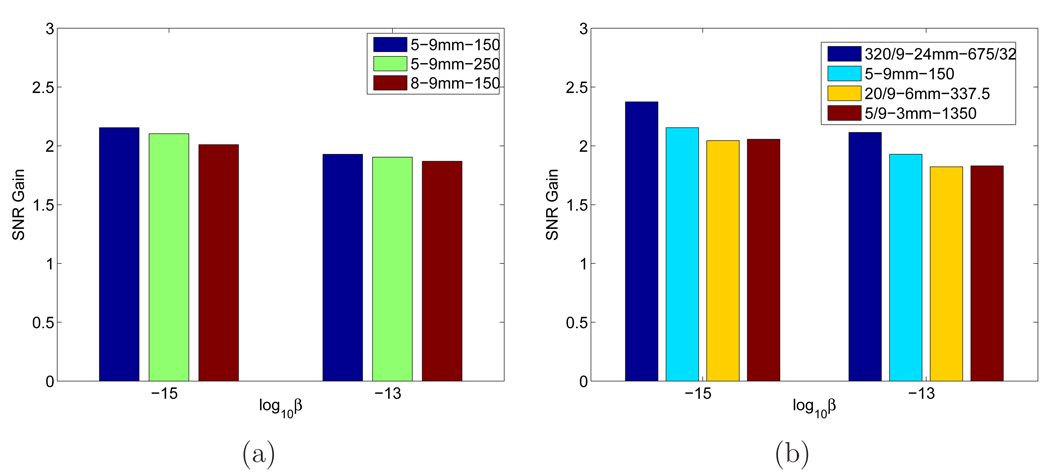
where G(σ2, rk) is a Gaussian blob with variance σ2 centered at a random location rk which was uniformly distributed within the phantom, K represents the total number of blobs, which is a Poisson random variable with mean Kmean, b represents the amplitude of the blob. Assuming that the constant background has an amplitude of b0, we considered 6 parameter combinations to represent different lumpiness: (a) b/b0 = 5, σ = 9 mm, Kmean = 150; (b) b/b0 = 5, σ = 9 mm, Kmean = 250; (c) b/b0 = 8, σ = 9 mm, Kmean = 150; (d) b/b0 = 320/9, σ = 24 mm, Kmean = 675/32; (e) b/b0 = 20/9, σ = 6 mm, Kmean = 337.5; and (f) b/b0 = 5/9, σ = 3 mm, Kmean = 1350. The first three cases (a–c) share the same correlation length (σ in Equation (28)) but different variance (the diagonal elements of Σx), while the first and the last three cases (a, d–f) have the same variance but different correlation. For each case, images were scaled to the same activity level as the example shown in Section 4.1 (with an expected number of true events of 579k). We added a hot lesion of diameter 12 mm at the center with an activity-background ratio of 3 : 2. Examples of these lumpy backgrounds are shown in Figure 19.
Figure 19.
Examples of lumpy backgrounds with different parameters. (a) b/b0 = 5, σ = 9 mm, Kmean = 150; (b) b/b0 = 5, σ = 9 mm, Kmean = 250; (c) b/b0 = 8, σ = 9 mm, Kmean = 150; (d) b/b0 = 320/9, σ = 24 mm, Kmean = 675/32; (e) b/b0 = 20/9, σ = 6 mm, Kmean = 337.5; and (f) b/b0 = 5/9, σ = 3 mm, Kmean = 1350.
The theoretical SNRs of TOF PET and non-TOF PET were computed using equation (16) where Σx was estimated from 5000 samples. The theoretical SNR gains are plotted in Figure 20. We can see that with all other conditions being the same, the SNR gain for the lumpy background is smaller than the uniform background case, although the changes in SNR gain are less than the corresponding changes in the absolute SNR values. In Figure 20(a), we show the SNR gains for different lumpy backgrounds with the same correlation length (σ = 9 mm). We can see that with the same correlation length, the SNR gain reduces with larger number of patches and greater amplitudes (both increase the variance). Figure 20(b) gives the SNR gain for different lumpy backgrounds with the same variance. It shows that with the same variance, the SNR gain reduces with the correlation length. It reaches the minimum when the width of the lumps is close to the tumor size. While the difference between σ = 6 mm and σ = 3 mm cases are small, we found that the SNR gain increased substantially when we removed the correlation completely by setting all the off-diagonal elements in Σx to zero. These results indicate it is important to consider background variability in evaluating TOF PET.
Figure 20.
Theoretically computed SNR gains for different lumpy backgrounds: (a) with the same correlation length σ = 9 mm; (b) with the same variance. The three numbers in the legend are the values of the lumpy background parameters b/b0, σ, and Kmean, respectively.
5. Conclusions
In this paper, we present a theoretical approach to investigate the performance of TOF PET in improving the lesion detectability. We used the list-mode MAP reconstruction and assessed the detection performance using the channelized Hotelling observer. We showed that the TOF PET provides better lesion detection performance than the non-TOF PET and the SNR gain is greater with higher random fraction, better system timing resolution, and larger patient. The scatters by themselves have little impact on the SNR gain after correction. Since the true system timing resolution may not be known precisely in practice, we investigated the effect of mismatched timing kernels and showed that using a mismatched timing kernel in reconstruction always degrades the detection performance, no matter whether it is narrower or wider than the real value. Using the proposed theoretical framework, we also studied the effect of background variability on the detection performance. Our results indicated that with lumpy background, the TOF PET still outperforms non-TOF PET, but the improvement is smaller compared with the uniform background case. More specifically, with the same correlation length, the SNR gain reduces with bigger number of lumpy patches and larger lumpy amplitudes. With the variance being equal, the SNR gain reaches the minimum when the width of the lumps is close to the size of the tumor. We plan to apply the analysis to real data in future work.
Acknowledgments
This work is supported in part by the Director, Office of Science, Office of Biological and Environmental Research, Medical Science Division of the U.S. Department of Energy under Contract No. DE-AC02-05CH11231, and in part by the National Institutes of Health, National Institute of Biomedical Imaging and Bioengineering under grant number R01-EB006085 and R01EB000194.
Reference
- 1.Moses W. Time-of-flight in PET revisited. IEEE Tran. Nucl. Sci. 2003;50:2325–2330. [Google Scholar]
- 2.Moses WW, Janecek M, Spurrier MA, Szupryczynski P, Choong W-S, Melcher CL, Andreaco M. Optimization of a LSO-Based Detector Module for Time-of-Flight PET. IEEE Trans. Nucl. Sci. 2010 doi: 10.1109/TNS.2010.2047266. in press. [DOI] [PMC free article] [PubMed] [Google Scholar]
- 3.Conti M, Bendriem B, Casey M, Chen M, Kehren F, Michel C, Panin V. First experimental results of time-of-flight reconstruction on an LSO PET scanner. Phys. Med. Biol. 2006;50:4507–4526. doi: 10.1088/0031-9155/50/19/006. [DOI] [PubMed] [Google Scholar]
- 4.Surti S, Huhn A, Werner M, Perkins A, Kolthammer J, Karp J. Performance of Philips Germini TF PET/CT scanner with special consideration for its time-of-flight imaging capabilities. J. Nucl. Med. 2007;48:471–480. [PubMed] [Google Scholar]
- 5.Karp J, Surti S, Daube-Witherspoon M, Muehllehner G. Benefit of time-of-flight in PET: Experimental and clinical results. J. Nucl. Med. 2008;49:462–470. doi: 10.2967/jnumed.107.044834. [DOI] [PMC free article] [PubMed] [Google Scholar]
- 6.Synder D, Thomas L, Jr, Ter-Pogossian M. A mathematical model for positron-emission tomography systems having time-of-flight measurements. IEEE Tran. Nucl. Sci. 1981;28:3575–3583. [Google Scholar]
- 7.Tomitani T. Image reconstruction and noise evaluation in photon time-of-flight assisted positron emission tomography. IEEE Tran. Nucl. Sci. 1981;28:4852–4859. [Google Scholar]
- 8.Harrison R, Alessio A, Kinahan P, Lewellen T. Signal to noise ratio in simulations of time-of-flight positron emission tomography. Conf. Record of the 2004 Nucl. Sci. Symp. and Med. Imaging Conf.; 2004. pp. 4080–4083. [Google Scholar]
- 9.Kimdom J, Qi J, Moses WW. Effect of random and scatter fractions in variance reduction using time-of-flight information. Conf. Record of the 2004 Nucl. Sci. Symp. and Med. Imaging Conf.; 2004. pp. 2571–2573. [Google Scholar]
- 10.Conti M. Effect of randoms on signal-to-noise-ratio in TOF PET. IEEE Tran. Nucl. Sci. 2006;53:1188–1193. [Google Scholar]
- 11.Lois C, Jakoby BW, Long MJ, Hubner KF, Barker DW, Casey ME, Conti M, Panin VY, Kadrmas DJ, Townsend DW. An assessment of the impact of incorporating time-of-flight information into clinical PET/CT imaging. J. Nucl. Med. 2010;51:237–245. doi: 10.2967/jnumed.109.068098. [DOI] [PMC free article] [PubMed] [Google Scholar]
- 12.Tewellen TK, Harrison RL, Vannoy S. The SimSET program, in Monte Carlo calculations. Monte Carlo Calculations in Nuclear Medicine. 1998:77–92. [Google Scholar]
- 13.Surti S, Karp J. Experimental evaluation of a simple lesion detection task with time-of-flight pet. Phys. Med. Biol. 2009;54:373–384. doi: 10.1088/0031-9155/54/2/013. [DOI] [PMC free article] [PubMed] [Google Scholar]
- 14.Kadrmas DJ, Casey ME, Conti M, Jakoby BW, Lois C, Townsend DW. Impact of time-of-flight on PET tumor detection. J. Nucl. Med. 2009;50:1315–1323. doi: 10.2967/jnumed.109.063016. [DOI] [PMC free article] [PubMed] [Google Scholar]
- 15.Vunckx K, Zhou L, Matej S, Defrise M, Nuyts J. Fisher infomration-based evaluation of image quality for time-of-flight PET. IEEE Tran. Med. Imaging. 2010;29:311–321. doi: 10.1109/TMI.2009.2029098. [DOI] [PMC free article] [PubMed] [Google Scholar]
- 16.Huesman RH, Klein G, Moses W, Qi J, Reutter B, Virador P. List-mode maximum-likelihood reconstruction applied to positron emission mammography (PET) with irregular sampling. IEEE Tran. Med. Imaging. 2000;19:532–537. doi: 10.1109/42.870263. [DOI] [PubMed] [Google Scholar]
- 17.Yao J, Barrett HH. Predicting human performance by a channelized hotelling model. Proc. SPIE. 1992;1768:161–168. [Google Scholar]
- 18.Oldan J, Kulkarni S, Xing Y, Khurd P, Gindi G. Channelized hotelling and human observer study of optimal smoothing in spect map reconstruction. IEEE Tran. Nucl. Sci. 2004;51:733–741. [Google Scholar]
- 19.Qi J. Analysis of lesion detectability in bayesian emission reconstruction with nonstationary object variability. IEEE Trans. Med. Imaging. 2004;23:321–329. doi: 10.1109/TMI.2004.824239. [DOI] [PubMed] [Google Scholar]
- 20.Qi J, Leahy RM. Resolution and noise properties of MAP reconstruction for fully 3D PET. IEEE Tran. Med. Imaging. 2000;19:493–506. doi: 10.1109/42.870259. [DOI] [PubMed] [Google Scholar]
- 21.Fessler JA, Rogers JL. Spatial resolution properties of penalized likelihood image reconstruction: Space-invariant tomographs. IEEE Tran. Image Process. 1996;5:1346. doi: 10.1109/83.535846. [DOI] [PubMed] [Google Scholar]
- 22.Vunckx K, Bequ D, Defrise M, Nuyts J. Single and multipinhole collimator design evaluation method for small animal SPECT. IEEE Tran. Med. Imag. 2008;27:36–46. doi: 10.1109/TMI.2007.902802. [DOI] [PubMed] [Google Scholar]
- 23.Stayman JW, Fessler JA. Compensation for nonuniform resolution using penalized-likelihood reconstruction in space-variant imaging systems. IEEE Tran. Med. Imag. 2004;23:269–284. doi: 10.1109/TMI.2003.823063. [DOI] [PubMed] [Google Scholar]
- 24.Johnson RJ, Johnson JJ, Rodriguez D, Tolimieri R. A methodology for designing, modifying, and implementing Fourier transform algorithms on various architectures. J. Circ. Sys. Signal. Proc. 1990:9. [Google Scholar]
- 25.Swensson R. Unified measurement of observer performance in detecting and localizing target objects on images. Med. Phys. 1996;23:1709–1725. doi: 10.1118/1.597758. [DOI] [PubMed] [Google Scholar]
- 26.Zubal IG, Harrell CR, Smith EO, Rattner Z, Gindi G, Hoffer PB. Computerized three-dimensional segmented human anatomy. Med. Phys. 1994;21:299–302. doi: 10.1118/1.597290. [DOI] [PubMed] [Google Scholar]
- 27.Rolland JP, Barrett HH. Effect of random background inhomogenerity on observer detection performance. J. Opt. Soc. Amer. A. 1992;9:649–658. doi: 10.1364/josaa.9.000649. [DOI] [PubMed] [Google Scholar]


