Potential for Bias in Case-Crossover Studies With Shared Exposures Analyzed Using SAS

Abstract

The case-crossover method is an efficient study design for evaluating associations between transient exposures and the onset of acute events. In one common implementation of this design, odds ratios are estimated using conditional logistic or stratified Cox proportional hazards models, with data stratified on each individual event. In environmental epidemiology, where aggregate time-series data are often used, combining strata with identical exposure histories may be computationally convenient. However, when the SAS software package (SAS Institute Inc., Cary, North Carolina) is used for analysis, users can obtain biased results if care is not taken to properly account for multiple cases observed at the same time. The authors show that fitting a stratified Cox model with the “Breslow” option for handling tied failure times (i.e., ties = Breslow) provides unbiased health-effects estimates in case-crossover studies with shared exposures. The authors’ simulations showed that using conditional logistic regression—or equivalently a stratified Cox model with the “ties = discrete” option—in this setting leads to health-effect estimates which can be biased away from the null hypothesis of no association by 22%–39%, even for small simulated relative risks. All methods tested by the authors yielded unbiased results under a simulated scenario with a relative risk of 1.0. This potential bias does not arise in R (R Foundation for Statistical Computing, Vienna, Austria) or Stata (Stata Corporation, College Station, Texas).

The case-crossover design is used to evaluate associations between transient exposures and the onset of acute events (1). In one common implementation of this design, each subject's exposure before a case-defining event (case period) is compared with his or her own exposure experience during 1 or more control periods in which the subject did not become a case. The use of matched, within-subject comparisons provides effective control of confounding by measured or unmeasured subject characteristics that are stable over time, although confounding by time-varying characteristics or exposures is still possible (1, 2). This implementation of the case-crossover design is analogous to a matched case-control study, and the odds ratio estimated with conditional logistic regression—or equivalently the stratified Cox proportional hazards model—is typically used as the measure of association.

Case-crossover methods have been applied to studies in a number of different substantive areas, including pharmacoepidemiology (3–6), cardiovascular disease (7–10), injury (11–14), infectious disease (15–17), and environmental epidemiology (18–20). The application of case-crossover methods is a common approach in studies evaluating the association between short-term changes in levels of ambient air pollutants and the risk of acute morbid or fatal events (8, 21–24). In this setting, it is common to assign the same exposure history to all persons experiencing the event of interest on a given day. In theory, case-crossover analyses should treat each event as a separate stratum in the analysis. In settings where exposure is shared, it is often convenient to condition the analysis on calendar day rather than the individual. Because conditioning on day allows data to be aggregated into fewer strata, analytic data sets are smaller and computation time can be reduced substantially. However, we show that when the analyses are performed using the SAS statistical software package, version 9.2 (SAS Institute Inc., Cary, North Carolina), failure to properly account for this aggregation can lead to health-effects estimates that are biased away from the null hypothesis of no association. Our goal in this paper is to characterize the magnitude, direction, and conditions under which this potential bias occurs.

MATERIALS AND METHODS

Suppose that one wants to evaluate the relation between levels of ambient fine particles (particulate matter with an aerodynamic diameter ≤2.5 μm (PM_2.5)) and the risk of hospitalization for a specific cause. The left side of Table 1 shows how one might structure the data set for a time-stratified case-crossover study. In this design, PM_2.5 levels at the time of each event are compared with PM_2.5 levels during referent periods sampled from other times in the same calendar month (25, 26). In this example, we assume that data are available on the date (but not the time) of each event, and we match case periods and referent periods on day of the week, but neither is necessary to the method or to our demonstration. Each event has a unique identifier. As is typical in this type of study, the same value of PM_2.5 is assigned to all events that occur at the same time.

Table 1.

Sample Data Set Structure for a Case-Crossover Analysis Conditioning on Each Individual (Left) or Conditioning on Each Calendar Day (Right) (n = 4 cases)^a

Row	Conditioning on Event ID					Conditioning on Day
	Event IDb	Datec	Daily PM2.5	Cased	Timee	Countf	Datec	Daily PM2.5	Cased	Timee
1	1	January 1, 2000	26.3	1	1	2	January 1, 2000	26.3	1	1
2	1	January 1, 2000	16.0	0	2	2	January 1, 2000	16.0	0	2
3	1	January 1, 2000	19.3	0	2	2	January 1, 2000	19.3	0	2
4	1	January 1, 2000	26.6	0	2	2	January 1, 2000	26.6	0	2
5	1	January 1, 2000	28.5	0	2	2	January 1, 2000	28.5	0	2
6	2	January 1, 2000	26.3	1	1	3	January 2, 2000	27.4	1	1
7	2	January 1, 2000	16.0	0	2	3	January 2, 2000	19.7	0	2
8	2	January 1, 2000	19.3	0	2	3	January 2, 2000	28.3	0	2
9	2	January 1, 2000	26.6	0	2	3	January 2, 2000	24.0	0	2
10	2	January 1, 2000	28.5	0	2	3	January 2, 2000	22.5	0	2
11	3	January 2, 2000	27.4	1	1
12	3	January 2, 2000	19.7	0	2
13	3	January 2, 2000	28.3	0	2
14	3	January 2, 2000	24.0	0	2
15	3	January 2, 2000	22.5	0	2
16	4	January 2, 2000	27.4	1	1
17	4	January 2, 2000	19.7	0	2
18	4	January 2, 2000	28.3	0	2
19	4	January 2, 2000	24.0	0	2
20	4	January 2, 2000	22.5	0	2
21	5	January 2, 2000	27.4	1	1
22	5	January 2, 2000	19.7	0	2
23	5	January 2, 2000	28.3	0	2
24	5	January 2, 2000	24.0	0	2
25	5	January 2, 2000	22.5	0	2

Abbreviations: ID, identifier; PM_2.5, particulate matter with an aerodynamic diameter ≤2.5 μm.

^aAll cases that occur on the same calendar day are assumed to involve exposure to the same levels of PM_2.5. Controls are chosen according to the time-stratified approach, such that all days in the same month and on the same day of the week as the case day are used as control days.

^bUnique individual identifier.

^cCalendar day during follow-up.

^d1 if case day, 0 if control days.

^e1 if case day, 2 if control days.

^fNumber of cases that occurred on that day.

We use conditional logistic regression, stratifying on each event, to estimate the association between PM_2.5 and the risk of hospitalization. In SAS, we can implement this analysis using the PHREG procedure as follows.

PROC PHREG data = expanded;

 MODEL time × case(0) = pm25 covariate₁…covariate_p/ties = Breslow;

 STRATA eventid;

run;

The MODEL statement describes the regression model to be fitted and the STRATA statement denotes that the analysis is conditioned on each individual event. Note that as part of the MODEL statement, SAS enables the user to specify how tied failure times will be handled in the analysis (e.g., ties = Breslow). However, since we are conditioning on each event (i.e., there is exactly 1 case in each stratum), there are no ties and all of the available ties-handling options yield exactly the same answer. Equivalently, one could use SAS's LOGISTIC procedure to fit the conditional logistic regression model as follows:

PROC LOGISTIC data = expanded;

 MODEL case = pm25 covariate₁…covariate_p;

 STRATA eventid;

run;

Since all events that occur at the same time are assigned the same exposure value, an attractive alternative approach is to create a data set with 1 stratum per calendar day and to weight each observation by the number of cases observed on that day (see right side of Table 1). We can implement this weighted analysis in SAS as follows:

PROC PHREG data = weighted;

 MODEL time*case(0) = pm25 covariate₁… covariate_p/ties = Breslow;

 STRATA date;

 FREQ count;

run;

In this case, the PHREG procedure treats each observation as if it appears n times, where n is the value of the FREQ variable for the observation. Since in this example we are conditioning on strata defined by calendar day, each stratum contains n_d events, where n_d may be more than 1. This approach is attractive because the analysis is computationally much faster, since there are many fewer strata. For large data sets, the difference in computation times can be substantial.

Now the approach used to handle tied failure times matters, since each stratum can contain multiple events. The default ties-handling option uses the approach described by Breslow (27), which maximizes a partial likelihood function that is identical to the partial likelihood function for the case-crossover design, as previously described (25, 26, 28) and as shown in the Appendix. However, the SAS manuals advise that when the PHREG procedure is being used to implement conditional logistic regression models (such as when analyzing data from a matched case-control study), the “discrete” ties-handling option should be used (29). As is shown in the Appendix, this construction differs from that which assumes independence across all matched sets in the case-crossover design. Therefore, the partial likelihood function generated from the “discrete” ties option differs from the correct partial likelihood function for case-crossover analyses, suggesting that use of the “discrete” option with the PHREG procedure may lead to biased effect estimates. However, the direction and magnitude of this potential bias are not clear.

Alternatively, we could use SAS's LOGISTIC procedure to fit the conditional logistic model incorporating the weights as follows:

PROC LOGISTIC data = weighted;

 MODEL case = pm25 covariate₁…covariate_p;

 STRATA date;

 FREQ count;

run;

This yields effect estimates identical to those of the PHREG procedure with the “ties = discrete” option but is computationally less efficient. The partial likelihood maximized by the LOGISTIC procedure with the frequency weights again differs from the correct partial likelihood function for case-crossover analyses.

Simulation studies

We performed simulations to quantify the direction and magnitude of the bias that results when the ties-handling procedure is incorrectly specified for a typical time-series study of air pollution health effects. First, we simulated the number of cause-specific hospital admissions on day i (Y_i) over a 10-year period as a Poisson random variable:

where PM_i represents PM_2.5 levels on day i and β₁ represents the hypothesized log rate ratio associated with a 1-μg/m³ increase in PM_2.5 on the same day. For PM_i, we simulated a time series of daily measures of PM_2.5 where the natural log of the exposure was normally distributed with a mean of 2.58 and a standard deviation of 0.54. These values were those observed in Chicago, Illinois, between 2000 and 2006 and were used in the applied example below. β₀ was chosen such that the mean number of events at the average PM_2.5 level was 5. Second, for each simulated data set, we evaluated the association between same-day PM_2.5 and risk of hospitalization using the time-stratified case-crossover design (25, 26), where referents were all days in the same year, month, and day of the week as the simulated case day, excluding the case day.

We simulated data sets for true rate ratios ranging from 0.80 to 2.00 per 10-μg/m³ increase in PM_2.5, including the null hypothesis of no association (rate ratio = 1.0). We used SAS's PHREG procedure with either the “Breslow” or the “discrete” ties-handling option to estimate odds ratios and 95% confidence intervals. We stratified on calendar day in all analyses. For each effect size, we simulated results for 250 data sets, and we report the average and the relative bias, defined as 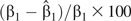The simulated data sets were created in R, version 2.7.2 (30), and exported into SAS for analysis.

Applied example

As an applied example, we evaluated the association between daily PM_2.5 and the risk of hospital admission for congestive heart failure among Medicare beneficiaries aged ≥65 years residing in the Chicago metropolitan area between January 1, 2000, and December 31, 2006. We obtained hospital admission records from the Centers for Medicare and Medicaid Services and defined cases as patients admitted from the emergency department with a primary discharge diagnosis of heart failure (International Classification of Diseases, Ninth Revision, code 428). We obtained daily measures of PM_2.5 from the Environmental Protection Agency and computed daily mean concentrations, as previously described (19). We obtained meteorologic data from the National Weather Service (National Climatic Data Center, Asheville, North Carolina). Finally, we evaluated the association between PM_2.5 and same-day risk of hospital admission using the time-stratified case-crossover design as above. We used SAS's PHREG procedure with either the “Breslow” or the “discrete” ties-handling option to estimate odds ratios and 95% confidence intervals. In all models, we controlled for confounding by temperature and dew point. This analysis was approved by the institutional review boards of the Harvard School of Public Health (Boston, Massachusetts) and Beth Israel Deaconess Medical Center (Boston, Massachusetts).

RESULTS

Simulation studies

Figure 1 shows the results of using SAS to analyze simulated data sets. Use of the “Breslow” ties-handling option when stratifying on day resulted in unbiased estimates of the simulated associations between PM_2.5 and same-day hospital admissions. As expected, when the “Breslow” ties option was used, results were identical regardless of whether we conditioned on each individual event or conditioned on calendar day weighted by the number of cases per day. However, using the “discrete” ties option, conditioning on calendar day, and weighting by the number of cases per day resulted in estimates that were potentially biased away from the null hypothesis of no association. Specifically, when the simulated relative risk differed from 1.0, effect estimates were biased by 22%–39% away from the null hypothesis. Using SAS's LOGISTIC procedure conditioned on calendar day and weighted by the number of cases per day yielded identical (biased) results. Under the simulated null hypothesis of no association, all methods yielded unbiased estimates.

Figure 1.

Results of analyses performed in SAS for simulated relative risks of hospitalization for heart failure ranging from 0.8 to 2.0 per 10-μg/m³ increase in particulate matter with an aerodynamic diameter ≤2.5 μm. Box plots show the distribution of effect estimates from 250 simulated data sets. Each box denotes the median value and interquartile range (25th–75th percentiles), and whiskers denote the upper and lower adjacent values. The vertical dashed lines denote the simulated relative risk.

Applied example

We evaluated the association between ambient PM_2.5 and the risk of hospitalization for congestive heart failure among Medicare beneficiaries residing in Chicago using the time-stratified case-crossover design (Table 2). Using SAS's PHREG procedure with the “Breslow” ties option and conditioning on each event, we observed a 1.2% (95% confidence interval: 0.1, 2.4) increase in risk of hospitalization for heart failure per 10-μg/m³ increase in PM_2.5. Conditioning on calendar day but still using the “Breslow” ties option yielded identical results. However, conditioning on calendar day and using the “discrete” ties option, we found a 1.6% (95% confidence interval: 0.3, 2.9) increase in risk of hospitalization per 10-μg/m³ increase in PM_2.5, representing a 30% relative bias away from the null on the log odds scale.

Table 2.

Association Between Ambient PM_2.5 and Risk of Hospitalization for Congestive Heart Failure, Estimated With Different SAS^a Procedures, Ties-Handling Options, and Frequency Weights, Among Medicare Beneficiaries Residing in Chicago, Illinois, 2000–2006

SAS Procedure	Ties Option	Conditioning On:	Weighted By:	Estimate, %b	95% Confidence Interval	Computational Time, seconds
PHREG	Breslowc	Each event		1.2	0.1, 2.4	18.3
PHREG	Breslow	Each day	Events/day	1.2	0.1, 2.4	0.8
PHREG	Discrete	Each day	Events/day	1.6	0.3, 2.9	9.3
LOGISTIC		Each event		1.2	0.1, 2.4	6.2
LOGISTIC		Each day	Events/day	1.6	0.3, 2.9	25.5

Abbreviation: PM_2.5, particulate matter with an aerodynamic diameter ≤2.5 μm.

^aSAS Institute Inc., Cary, North Carolina.

^bPercentage increase in risk of hospitalization for heart failure per 10-μg/m³ increase in PM_2.5.

^cAny of the available ties-handling options would yield identical results in this case.

Analysis of the weighted data set using the LOGISTIC procedure yielded (biased) estimates identical to those observed with the PHREG procedure using the “discrete” ties option, but took almost 3 times longer (25.5 seconds vs. 9.3 seconds). The PHREG procedure using the “Breslow” ties-handling option took 0.8 seconds to execute.

DISCUSSION

The case-crossover study design has been applied in a large number of epidemiologic studies, and its use is common in studies of the health effects of environmental exposures. It has been shown that when an appropriate control selection strategy is used, conditional logistic regression stratified on the individual subject yields unbiased estimates of the relative risk (25, 26). When analyses are stratified on the individual, there are no tied failure times, and all of the commonly available partial likelihoods (i.e., ties options) reduce to the same valid partial likelihood function. However, when multiple subjects are assigned a common exposure history, it is computationally advantageous to group subjects with identical exposure histories and condition on each group rather than each individual event. Because of the analogy between case-crossover and matched case-control studies—and by extension, Cox proportional hazards analysis of time-to-event data—we suspect that some investigators may use the discrete partial likelihood, as suggested by the software manuals, to mimic the likelihood function used in conditional logistic regression (29, 31). Other investigators may be using SAS's LOGISTIC procedure, conditioning on each calendar day and weighting the analysis by the number of cases observed per day. Our results show that use of these approaches in SAS will result in estimates that are biased away from the null hypothesis of no association. Results from our simulations demonstrate that the relative magnitude of this bias can be substantial even for small effect sizes.

Notably, these results do not imply that there is a problem with SAS's implementation of the PHREG or LOGISTIC procedures, the handling of tied failure times, or the handling of frequency weights. Rather, as the Appendix shows, because of how these SAS procedures incorporate frequency weights into the analysis, the partial likelihood function fitted by SAS is not the correct one for case-crossover analyses with shared exposures. Stata (Stata Corporation, College Station, Texas) and R (R Foundation for Statistical Computing, Vienna, Austria) are not prone to this bias because of the way in which each of these software packages incorporates frequency weights into the analysis. Recall that SAS's FREQ statement treats each observation as if it appeared in the data set n times. This is equivalent to manually replicating each row in the data set n times. In contrast, Stata's clogit function incorporates frequency weights directly into the partial likelihood function and therefore yields unbiased estimates. In R, the clogit function of the “survival” package does not allow weights to be used. Neither the coxph function in R nor the stcox function in Stata allows the use of weights when the exact partial likelihood function is specified for handling tied failure times (the “exact” option in R and the “exactp” option in Stata). Therefore, this potential bias arises in SAS only because of the particular manner in which SAS implements the FREQ statement.

Thus, we recommend that SAS users wishing to collapse strata with identical exposure histories use the PHREG procedure with the “Breslow” ties-handling option. A weighted analysis using SAS's LOGISTIC procedure or using the PHREG procedure with the “discrete” ties option will lead to biased results. Of course, it must be emphasized that using an expanded data set (as in Table 1) and conditioning on each individual event yields unbiased estimates with any of these procedures. Even so, for large data sets the PHREG procedure may be preferable to the LOGISTIC procedure because of computational efficiency. For very large data sets, such as those typically used in recent studies (32–34), the computational time needed to use the LOGISTIC procedure may be problematic. Investigators in recent studies have performed similar analyses in more than 200 cities, such that even with today's high-performance computers, the difference in computational time may be important.

Since few published articles describe the statistical implementation of the conditional logistic regression model, it is difficult to know how prevalent this error is in the published literature. However, examples can be found in both published research articles and publicly available presentations, suggesting that at least some researchers and educators are confused as to the appropriate approach.

The potential problem identified here is not unique to studies of air pollution health effects. Shared exposures are common in other areas of environmental epidemiology, including studies of the health effects of weather and climate (15, 19) and water quality (18), and in areas outside of environmental health, such as the health effects of alcohol sales (35), hospital nurse staffing levels (36), and air travel (37). As the popularity of the case-crossover method grows, it is important that investigators be aware of potential analytic pitfalls. Moreover, this potential problem may also arise in case-specular or case-control studies with shared or ecologic exposure information among cases.

Glossary

Abbreviation

PM_2.5

particulate matter with an aerodynamic diameter ≤2.5 μm

APPENDIX

The case-crossover study design compares the exposure of cases in interval t_i with the exposures from a set of reference periods. Using the notation of Lu and Zeger (28), we denote the event interval by t_i, the set of reference periods by W(t_i), and the exposure for subject i during the event interval as $X_{i{t}_i}$. Assuming that the n subjects are independent and that the baseline risk is constant within the reference window, the likelihood function is given by

(A1)

Taking account of the shared exposure for all events on a given day, $X_{i{t}_i}$ can be notationally represented by X_d, which represents the exposure associated with day d of the study. Using this notation, equation A1 is equivalent to

(A2)

where n_d denotes the number of cases observed on day d. Equation A2 is identical to the partial likelihood function used by the Breslow approach for handling tied failure times in the setting of the proportional hazards model (29).

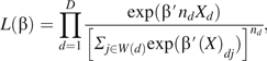
In contrast, the partial likelihood function specified by the “discrete” ties option in SAS (29) is given by

(A3)

where Q_d is the set of all possible collections of n_d cases from an expanded risk set constructed from n_d replications of the correct risk set W(d), and s_q is the sum of the exposures associated with the n_d cases in collection q. Generally, the denominators of equations A2 and A3 will not be equal, suggesting that use of the likelihood function shown in equation A3 will result in biased estimates of β.

References

- 1.Maclure M. The case-crossover design: a method for studying transient effects on the risk of acute events. Am J Epidemiol. 1991;133(2):144–153. doi: 10.1093/oxfordjournals.aje.a115853. [DOI] [PubMed] [Google Scholar]
- 2.Suissa S. The case-time-control design. Epidemiology. 1995;6(3):248–253. doi: 10.1097/00001648-199505000-00010. [DOI] [PubMed] [Google Scholar]
- 3.Barbone F, McMahon AD, Davey PG, et al. Association of road-traffic accidents with benzodiazepine use. Lancet. 1998;352(9137):1331–1336. doi: 10.1016/s0140-6736(98)04087-2. [DOI] [PubMed] [Google Scholar]
- 4.Confavreux C, Suissa S, Saddier P, et al. Vaccinations and the risk of relapse in multiple sclerosis. Vaccines in Multiple Sclerosis Study Group. N Engl J Med. 2001;344(5):319–326. doi: 10.1056/NEJM200102013440501. [DOI] [PubMed] [Google Scholar]
- 5.Olesen JB, Hansen PR, Erdal J, et al. Antiepileptic drugs and risk of suicide: a nationwide study. Pharmacoepidemiol Drug Saf. 2010;19(5):518–524. doi: 10.1002/pds.1932. [DOI] [PubMed] [Google Scholar]
- 6.Hallas J, Bjerrum L, Stovring H, et al. Use of a prescribed ephedrine/caffeine combination and the risk of serious cardiovascular events: a registry-based case-crossover study. Am J Epidemiol. 2008;168(8):966–973. doi: 10.1093/aje/kwn191. [DOI] [PMC free article] [PubMed] [Google Scholar]
- 7.Mittleman MA, Maclure M, Glasser DB. Evaluation of acute risk for myocardial infarction in men treated with sildenafil citrate. Am J Cardiol. 2005;96(3):443–446. doi: 10.1016/j.amjcard.2005.03.097. [DOI] [PubMed] [Google Scholar]
- 8.Levy D, Sheppard L, Checkoway H, et al. A case-crossover analysis of particulate matter air pollution and out-of-hospital primary cardiac arrest. Epidemiology. 2001;12(2):193–199. [PubMed] [Google Scholar]
- 9.Muller JE, Mittleman MA, Maclure M, et al. Triggering myocardial infarction by sexual activity. Low absolute risk and prevention by regular physical exertion. Determinants of Myocardial Infarction Onset Study Investigators. JAMA. 1996;275(18):1405–1409. doi: 10.1001/jama.275.18.1405. [DOI] [PubMed] [Google Scholar]
- 10.Baylin A, Hernandez-Diaz S, Siles X, et al. Triggers of nonfatal myocardial infarction in Costa Rica: heavy physical exertion, sexual activity, and infection. Ann Epidemiol. 2007;17(2):112–118. doi: 10.1016/j.annepidem.2006.05.004. [DOI] [PubMed] [Google Scholar]
- 11.Valent F, Di Bartolomeo S, Marchetti R, et al. A case-crossover study of sleep and work hours and the risk of road traffic accidents. Sleep. 2010;33(3):349–354. doi: 10.1093/sleep/33.3.349. [DOI] [PMC free article] [PubMed] [Google Scholar]
- 12.Chen SY, Fong PC, Lin SF, et al. A case-crossover study on transient risk factors of work-related eye injuries. Occup Environ Med. 2009;66(8):517–522. doi: 10.1136/oem.2008.042325. [DOI] [PubMed] [Google Scholar]
- 13.Möller J, Hallqvist J, Laflamme L, et al. Emotional stress as a trigger of falls leading to hip or pelvic fracture. Results from the ToFa study—a case-crossover study among elderly people in Stockholm, Sweden. BMC Geriatr. 2009;9:7. doi: 10.1186/1471-2318-9-7. (doi: 10.1186/1471-2318-9-7) [DOI] [PMC free article] [PubMed] [Google Scholar]
- 14.Gmel G, Kuendig H, Rehm J, et al. Alcohol and cannabis use as risk factors for injury—a case-crossover analysis in a Swiss hospital emergency department. BMC Public Health. 2009;9:40. doi: 10.1186/1471-2458-9-40. (doi: 10.1186/1471-2458-9-40) [DOI] [PMC free article] [PubMed] [Google Scholar]
- 15.Soverow JE, Wellenius GA, Fisman DN, et al. Infectious disease in a warming world: how weather influenced West Nile virus in the United States (2001–2005) Environ Health Perspect. 2009;117(7):1049–1052. doi: 10.1289/ehp.0800487. [DOI] [PMC free article] [PubMed] [Google Scholar]
- 16.Yang Z, Zhou F, Dorman J, et al. Association between infectious diseases and type 1 diabetes: a case-crossover study. Pediatr Diabetes. 2006;7(3):146–152. doi: 10.1111/j.1399-543X.2006.00163.x. [DOI] [PMC free article] [PubMed] [Google Scholar]
- 17.Dixon KE. A comparison of case-crossover and case-control designs in a study of risk factors for hemorrhagic fever with renal syndrome. Epidemiology. 1997;8(3):243–246. doi: 10.1097/00001648-199705000-00003. [DOI] [PubMed] [Google Scholar]
- 18.Ng V, Tang P, Jamieson F, et al. Going with the flow: legionellosis risk in Toronto, Canada is strongly associated with local watershed hydrology. Ecohealth. 2008;5(4):482–490. doi: 10.1007/s10393-009-0218-0. [DOI] [PubMed] [Google Scholar]
- 19.O'Neill MS, Zanobetti A, Schwartz J. Modifiers of the temperature and mortality association in seven US cities. Am J Epidemiol. 2003;157(12):1074–1082. doi: 10.1093/aje/kwg096. [DOI] [PubMed] [Google Scholar]
- 20.Tsai SS, Goggins WB, Chiu HF, et al. Evidence for an association between air pollution and daily stroke admissions in Kaohsiung, Taiwan. Stroke. 2003;34(11):2612–2616. doi: 10.1161/01.STR.0000095564.33543.64. [DOI] [PubMed] [Google Scholar]
- 21.Peel JL, Metzger KB, Klein M, et al. Ambient air pollution and cardiovascular emergency department visits in potentially sensitive groups. Am J Epidemiol. 2007;165(6):625–633. doi: 10.1093/aje/kwk051. [DOI] [PubMed] [Google Scholar]
- 22.Karr C, Lumley T, Shepherd K, et al. A case-crossover study of wintertime ambient air pollution and infant bronchiolitis. Environ Health Perspect. 2006;114(2):277–281. doi: 10.1289/ehp.8313. [DOI] [PMC free article] [PubMed] [Google Scholar]
- 23.Zeka A, Zanobetti A, Schwartz J. Individual-level modifiers of the effects of particulate matter on daily mortality. Am J Epidemiol. 2006;163(9):849–859. doi: 10.1093/aje/kwj116. [DOI] [PubMed] [Google Scholar]
- 24.Peters A, Dockery DW, Muller JE, et al. Increased particulate air pollution and the triggering of myocardial infarction. Circulation. 2001;103(23):2810–2815. doi: 10.1161/01.cir.103.23.2810. [DOI] [PubMed] [Google Scholar]
- 25.Lumley T, Levy D. Bias in the case-crossover design: implications for studies of air pollution. Environmetrics. 2000;11(6):689–704. [Google Scholar]
- 26.Levy D, Lumley T, Sheppard L, et al. Referent selection in case-crossover analyses of acute health effects of air pollution. Epidemiology. 2001;12(2):186–192. doi: 10.1097/00001648-200103000-00010. [DOI] [PubMed] [Google Scholar]
- 27.Breslow N. Covariance analysis of censored survival data. Biometrics. 1974;30(1):89–99. [PubMed] [Google Scholar]
- 28.Lu Y, Zeger SL. On the equivalence of case-crossover and time series methods in environmental epidemiology. Biostatistics. 2007;8(2):337–344. doi: 10.1093/biostatistics/kxl013. [DOI] [PubMed] [Google Scholar]
- 29.SAS Institute Inc. Example 64.5 . SAS/STAT 9.2 User's Guide. 2nd ed. Cary, NC: SAS Institute Inc; 2010. Conditional logistic regression for m: n matching. [Google Scholar]
- 30.R Development Core Team . R Foundation for Statistical Computing. Vienna: Austria; 2008. R: A Language and Environment for Statistical Computing. [Google Scholar]
- 31.Cleves MA, Gould WW, Gutierrez RG. An Introduction to Survival Analysis Using Stata. Revised Edition. College Station, TX: Stata Press; 2004. [Google Scholar]
- 32.Dominici F, Peng RD, Bell ML, et al. Fine particulate air pollution and hospital admission for cardiovascular and respiratory diseases. JAMA. 2006;295(10):1127–1134. doi: 10.1001/jama.295.10.1127. [DOI] [PMC free article] [PubMed] [Google Scholar]
- 33.Peng RD, Bell ML, Geyh AS, et al. Emergency admissions for cardiovascular and respiratory diseases and the chemical composition of fine particle air pollution. Environ Health Perspect. 2009;117(6):957–963. doi: 10.1289/ehp.0800185. [DOI] [PMC free article] [PubMed] [Google Scholar]
- 34.Bell ML, Ebisu K, Peng RD, et al. Seasonal and regional short-term effects of fine particles on hospital admissions in 202 US counties, 1999–2005. Am J Epidemiol. 2008;168(11):1301–1310. doi: 10.1093/aje/kwn252. [DOI] [PMC free article] [PubMed] [Google Scholar]
- 35.Ray JG, Moineddin R, Bell CM, et al. Alcohol sales and risk of serious assault. PLoS Med. 2008;5(5):e104. doi: 10.1371/journal.pmed.0050104. (doi: 10.1371/journal.pmed.0050104) [DOI] [PMC free article] [PubMed] [Google Scholar]
- 36.Hugonnet S, Villaveces A, Pittet D. Nurse staffing level and nosocomial infections: empirical evaluation of the case-crossover and case-time-control designs. Am J Epidemiol. 2007;165(11):1321–1327. doi: 10.1093/aje/kwm041. [DOI] [PubMed] [Google Scholar]
- 37.Schreijer AJ, Hoylaerts MF, Meijers JC, et al. Explanations for coagulation activation after air travel. J Thromb Haemost. 2010;8(5):971–978. doi: 10.1111/j.1538-7836.2010.03819.x. [DOI] [PubMed] [Google Scholar]