Is the Homunculus “Aware” of Sensory Adaptation?

Abstract

Neural activity and perception are both affected by sensory history. The work presented here explores the relationship between the physiological effects of adaptation and their perceptual consequences. Perception is modeled as arising from an encoder-decoder cascade, in which the encoder is defined by the probabilistic response of a population of neurons, and the decoder transforms this population activity into a perceptual estimate. Adaptation is assumed to produce changes in the encoder, and we examine the conditions under which the decoder behavior is consistent with observed perceptual effects in terms of both bias and discriminability. We show that for all decoders, discriminability is bounded from below by the inverse Fisher information. Estimation bias, on the other hand, can arise for a variety of different reasons and can range from zero to substantial. We specifically examine biases that arise when the decoder is fixed, “unaware” of the changes in the encoding population (as opposed to “aware” of the adaptation and changing accordingly). We simulate the effects of adaptation on two well-studied sensory attributes, motion direction and contrast, assuming a gain change description of encoder adaptation. Although we cannot uniquely constrain the source of decoder bias, we find for both motion and contrast that an “unaware” decoder that maximizes the likelihood of the percept given by the preadaptation encoder leads to predictions that are consistent with behavioral data. This model implies that adaptation-induced biases arise as a result of temporary suboptimality of the decoder.

1 Introduction

Sensory perception and the responses of sensory neurons are affected by the history of sensory input over a variety of timescales. Changes that occur over relatively short timescales (tens of milliseconds to minutes) are commonly referred to as adaptation effects, and have been observed in virtually all sensory systems. In the mammalian visual cortex, physiological recordings show that adaptation leads to a decrease in neurons’ responsivity, as well as other changes in tuning curves shapes and noise properties (see Kohn, 2007, for a review). In behavioral experiments, adaptation leads to illusory aftereffects (the best-known example is the waterfall illusion; Addams, 1834), as well as changes in the value and precision of attributes estimated from the visual input. Specifically, prolonged exposure to a visual stimulus of a particular orientation, contrast, or direction of movement induces a systematic bias in the estimation of the orientation (Gibson & Radner, 1937; Clifford, 2002), contrast (Hammett, Snowden, & Smith, 1994), or direction (Levinson & Sekuler, 1976) of subsequent stimuli. Adaptation also profoundly modulates the perceptual discrimination performance of these same variables (Regan & Beverley, 1985; Clifford, 2002).

From a normative perspective, it seems odd that the performance of sensory systems, which is generally found to be quite impressive, should be so easily disrupted by recent stimulus history. A variety of theoretical explanations for the observed neural effects have been proposed, including reduction of metabolic cost (Laughlin, de Ruyter van Steveninck, & Anderson, 1998), homeostatic remapping of dynamic range (Laughlin, 1981; Fairhall, Lewen, Bialek, & de Ruyter Van Steveninck, 2001), improvement of signal-to-noise ratio around the adapter (Stocker & Simoncelli, 2005), and efficient coding of information (Barlow, 1990; Atick, 1992; Wainwright, 1999; Wainwright, Schwartz, & Simoncelli, 2002; Langley & Anderson, 2007). On the perceptual side, explanations have generally centered on improvement of discriminability around the adapter (see Abbonizio, Langley, & Clifford, 2002), although the evidence for this is somewhat inconsistent. No current theory serves to fully unify the physiological and perceptual observations.

From a more mechanistic perspective, the relationship between the physiological and the perceptual effects also remains unclear. A number of authors have pointed out that repulsive biases are consistent with a fixed labeled-line readout of a population of cells in which some subset of the responses has been suppressed by adaptation (Blakemore & Sutton, 1969; Coltheart, 1971; Clifford, Wenderoth, & Spehar, 2000). More recent physiological measurements reveal that adaptation effects in neurons are often more varied and complex than simple gain reduction (Jin, Dragoi, Sur, & Seung, 2005; Kohn, 2007), and several authors have shown how some of these additional neural effects might contribute to perceptual after-effects (Jin et al., 2005; Schwartz, Hsu, & Dayan, 2007). In all of these cases, the authors examine how the neural effects of adaptation produce the perceptual effects, assuming a fixed readout rule for determining a percept from a neural population. Assuming such a fixed readout strategy corresponds to assuming implicitly that downstream decoding mechanisms are “unaware” of the adaptation-induced neural changes, thus becoming mismatched to the new response properties. This assumption has been explicitly discussed (Langley & Anderson, 2007) and referred to as a decoding ambiguity (Fairhall et al., 2001) or coding catastrophe (Schwartz et al., 2007). However, this “unaware” decoder assumption is at odds with the normative perspective, which typically assumes that the decoder should be “aware” of the postadaptation responses and adjust accordingly. Currently the solution adopted by the brain for the reading out of dynamically changing neural responses remains a mystery.

In this article, we re-examine the relationship between the physiological and psychophysical aspects of adaptation. We assume that perception can be described using an encoding-decoding cascade. The encoding stage represents the transformation between the external sensory stimuli and the activity of a population of neurons in sensory cortex, while the decoding stage represents the transformation from that activity to a perceptual estimate. We assume simple models of neural response statistics and adaptation at the encoding stage, and examine what type of optimal readout of the population activity is consistent with observed perceptual effects. In particular, we compare the behavior of aware and unaware decoders in explaining the perceptual effects of adaptation to motion direction and contrast. For each type of adaptation, we examine changes in the mean and variability of perceptual estimates resulting from adaptation, and we relate these to perceptually measurable quantities of bias and discriminability. We show that the Fisher information, which is widely used to compute lower bounds on the variance of unbiased estimators and has been used to assess the impact of adaptation on the accuracy of perceptual representations (Dean, Harper, & McAlpine, 2005; Durant, Clifford, Crowder, Price, & Ibbotson, 2007; Schwartz et al., 2007; Gutnisky & Dragoi, 2008), can also be used to compute a bound on perceptual discrimination thresholds, even in situations where the estimator is biased. Our results are consistent with the notion that simple models of neural adaptation, coupled with an unaware readout, can account for the main features of the perceptual behavior.

2 Encoding-Decoding Model

We define the relationship between physiology and psychophysics using an encoding-decoding cascade. We make simplifying assumptions. In particular, we assume that perception of a given sensory attribute is gated by a single, homogeneous population of neurons whose responses vary with that attribute, and we assume that the full population is arranged so as to cover the full range of values of that attribute.

2.1 Encoding

Consider a population of N sensory neurons responding to a single attribute of a stimulus s (e.g., the direction of motion of a moving bar). On a given stimulus presentation, the response of each neuron is a function of the neuron’s tuning curve and the neuron’s variability from trial to trial. For example, if the tuning curves are denoted f_i (s) and the variability is gaussian and independent, the response of neuron i can be written as

$$r_i=f_i(s)+{\eta }_i,$$ (2.1)

where the η_i’s are independent gaussian random variables. The population response to stimulus s is described by the probability density P(r | s), where r = {r₁, r₂…, r_N} is the vector of the spike counts of all neurons on each trial. The encoding process is fully characterized by the conditional density P(r | s), which, when interpreted as a function of s, is known as the likelihood function.

2.2 Decoding

Decoding refers to the inverse problem: given the noisy response r, one wants to obtain an estimate ŝ(r) of the stimulus. A variety of decoders can be constructed, with different degrees of optimality and complexity.¹ In general, an optimal decoder is one that is chosen to minimize some measure of error. The selection of an optimal estimator depends on the encoder model, P(r | s). A common choice in the population coding literature is the maximum likelihood (ML) estimator, ŝ(r) = arg max_s P(r | s). Another common choice is the minimum mean squared error (MMSE) estimator, ŝ(r) = 〈s | r〉, the conditional mean of the stimulus given the neural responses. Note that the ensemble of stimuli over which the mean is taken is part of the definition of optimality. Some common suboptimal examples include the population vector decoder² (the sum of the responses, weighted by the label of each neuron, divided by the sum of responses) (Georgopoulos, Schwartz, & Kettner, 1986) and the winner-takes-all decoder (which chooses the label associated with the neuron with the strongest response).

It is common to assess the quality of a decoder based on two quantities: the bias b(s) and the variance σ ²(s). The bias is the difference between the average of ŝ(r) across trials that use the stimulus s and the true value of s:

$$b(s)=\langle \widehat{s}(\mathbf{r})\rangle -s,$$ (2.2)

where the angle brackets again indicate an average over the responses, r, conditioned on the stimulus, s. An estimator is termed unbiased if b(s) = 0 for all stimulus values. The variance of the estimator, which quantifies how much the estimate varies about its mean value, is defined as

$${\widehat{\sigma }}^2(s)=\langle {[\widehat{s}(\mathbf{r})-\langle \widehat{s}(\mathbf{r})\rangle ]}^2\rangle .$$ (2.3)

The bias and the variance can be used to compute the trial average squared estimation error:

$$E(s)=\langle {(\widehat{s}(\mathbf{r})-s)}^2\rangle ={\sigma }^2(s)+b^2(s).$$ (2.4)

Thus, for an unbiased estimator, the average squared estimation error is equal to the variance. The ML estimator is often used because it is, under mild assumptions, asymptotically (i.e., in the limit of infinite data) unbiased and minimal in variance (Kay, 1993).

2.3 Aware and Unaware Decoders

During sensory adaptation, neurons’ tuning curves and response properties change, and thus the encoder model P(r | s) changes. But what about the decoder? Is it fixed, or does it also change during adaptation? As illustrated in Figure 1, two types of readout have been considered in adaptation studies. The first, common in the neural coding literature (Deneve, Latham, & Pouget, 1999; Xie, 2002; Jazayeri & Movshon, 2006), assumes that the decoder is optimized to match the encoder (typically, a maximum likelihood estimate is used). In order to maintain this optimality under adaptation, it must be aware of the changes in the encoder, and it must dynamically adjust to match those changes.³ This model, which we refer to as ŝ_aw(r), is often implicitly assumed in studies looking at the functional benefit of adaptation, in particular for discrimination performance. For example, a number of authors use the Fisher information to characterize neural responses before and after adaptation (Dean et al., 2005; Durant et al., 2007; Gutnisky & Dragoi, 2008). As detailed below, Fisher information is usually used to provide a bound on the accuracy of optimal (thus aware) population decoders.

Figure 1.

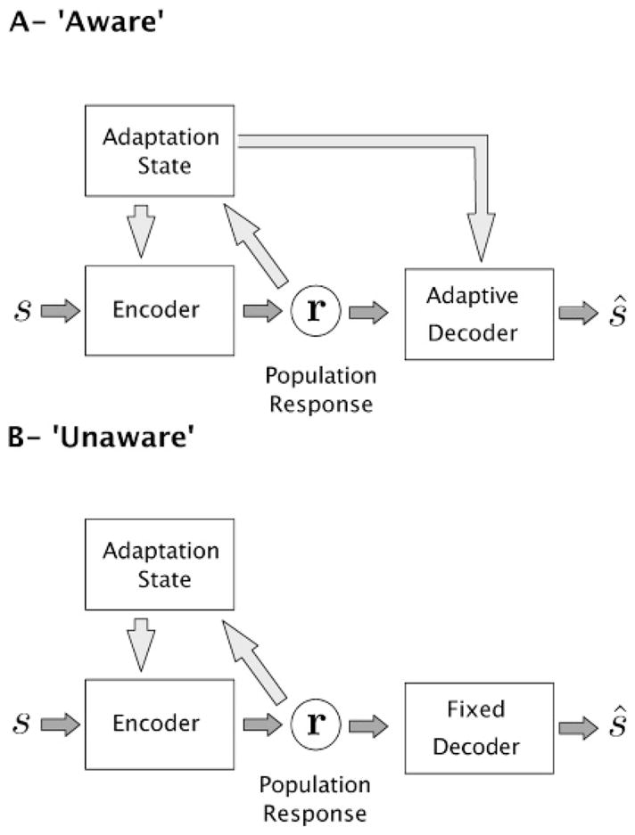
Encoding-decoding framework for adaptation. The encoder represents stimulus s using the stochastic responses of a neural population, r. This mapping is affected by the current adaptation state, and the responses can also affect the adaptation state. Two types of decoders can be considered. (A) An aware decoder knows of the adaptive state of the encoder and can adjust itself accordingly. Note that although the diagram implies that the adaptation state must be transmitted via a separate channel, it might also be possible to encode it directly in the population response. (B) An unaware decoder is fixed and ignores any adaptive changes in the encoder.

An aware decoder must have full knowledge of the adaptation-induced changes in the responses of the encoder. An alternative approach, found in much of the earlier literature on adaptation, assumes that the decoder is fixed and will thus be mismatched to the adapted encoder. Simple forms of this type of model have been successfully used to account for estimation biases induced by adaptation (Sutherland, 1961; Blakemore & Sutton, 1969; Coltheart, 1971; Clifford et al., 2000; Jin et al., 2005; Langley & Anderson, 2007). We will refer to any decoder that is unaffected by adaptive changes in the encoder as unaware, but we will be particularly interested in decoders that are chosen to be optimal prior to adaptation. For example, we could assume an unaware ML decoder, denoted ML_unaw, which selects as an estimate the stimulus that maximizes the probability of the observed response under the preadaptation encoding model P_pre(r | s).

In conclusion, two distinct types of decoder, “aware” and “unaware,” have been related to measures of discriminability or estimation, respectively: biases in estimation have typically been explained using fixed (and thus, unaware) decoders such as the population vector (see e.g., Jin et al., 2005), whereas discriminability has typically been studied using the Fisher information, which implicitly assumes an unbiased (and thus, in most cases, aware) estimator. However, no consistent account has been provided of both types of perceptual effect simultaneously. In the following, we examine both aware and unaware decoders, and we compare their behaviors to psychophysical measurements of both bias and discrimination.

3 Relating Decoder Behavior to Psychophysical Measurements

The output of the encoding-decoding cascade, as characterized by its estimation bias b(s) and variance σ̂²(s), represents the percept of the stimulus, which can be measured experimentally. We discuss in the following how estimation bias and variances relate to typical psychophysical measurements of bias and discriminability before and after adaptation.

3.1 Estimation Performance

Estimation biases are commonly measured by giving the subject a tool to indicate the perceived value of the stimulus parameter (e.g., by asking subjects to adjust an arrow pointing in the perceived direction of a moving stimulus) or by a two-alternative-forced-choice paradigm (2AFC) where subjects are asked to compare the stimulus with another stimulus presented in a control situation (e.g., at a nonadapted position). The parameter value of this control stimulus is then varied until the subject perceives both stimuli to be identical (point of subjective equality). Either procedure can be used to determine the estimation bias b(s).

3.2 Discrimination Performance

Discriminability is a measure of how well the subject can detect small differences in the stimulus parameter s. It is typically measured using a 2AFC paradigm. Discrimination performance is commonly summarized by the threshold (or just noticeable difference) (δs)_α, the amount by which the two stimuli must differ in parameter value s such that the subject answers correctly with probability P_correct = α.

In order to understand how the discrimination threshold is related to the bias b(s) and the variance σ̂²(s) of the estimator, consider the situation where two stimuli are present with parameters s₁ = s₀ − δs/2 and s₂ = s₀ + δs/2. The subject’s task is to assess which stimulus has the larger parameter value. Based on the noisy neural responses, the subject computes a parameter estimate for both stimuli, which we denote as ŝ₁ and ŝ₂.⁴ These estimates vary from trial to trial, forming distributions that we approximate by gaussians with mean μ̂(s) and standard deviation σ̂(s).

Signal detection theory (Green & Swets, 1966) may be extended (Stocker & Simoncelli, 2006) to describe how the subject’s probability of detecting the correct parameter difference between the two stimuli is related to the characteristics of the estimates:

$$P_{\mathit{correct}}(s_1,s_2)=\frac{1}{2}\text{erfc}\left(-\frac{D(s_1,s_2)}{2}\right),$$ (3.1)

where

$$\text{erfc}(x)=\frac{2}{\sqrt{\pi }}{\int }_{-\infty }^{x}d{ye}^{-y^2},$$ (3.2)

and D(s₁, s₂) is the normalized distance (often called d prime) between the distributions of the estimates ŝ₁ and ŝ₂, given as

$$D(s_1,s_2)=\frac{\widehat{\mu }(s_2)-\widehat{\mu }(s_1)}{\sqrt{\frac{{\widehat{\sigma }}^2(s_2)+{\widehat{\sigma }}^2(s_1)}{2}}}.$$ (3.3)

For small δs, we can assume that the variance of the two estimates is approximately the same. Writing μ̂ (s) = s + b(s), we can approximate D(s₁, s₂) as

$$D(s_0,\delta s)\approx \frac{\delta s(1+b^{\prime }(s_0))}{\widehat{\sigma }(s_0)},$$ (3.4)

where b′(s) is the derivative of the bias b(s).

For a given discrimination criterion α, equation 3.1 can be used to find the corresponding value D_α, (e.g., D_80% ≃ 1.4, and D_76% ≃ 1). The discrimination threshold (δs)_α is then obtained from equation 3.4 as

$${(\delta s)}_{\alpha }=D_{\alpha }\frac{\widehat{\sigma }(s_0)}{1+b^{\prime }(s_o)}.$$ (3.5)

The threshold is a function of both the standard deviation of the estimates and the derivative of the bias, as illustrated in Figure 2. Specifically, a positive bias derivative corresponds to an expansion of the perceptual parameter space (in the transformation from the stimulus space to the estimate space) and improves discriminability (decreases threshold), while a negative derivative corresponds to a contraction and decreases discriminability. Thus, adaptation-induced repulsive biases away from the adapter can improve discriminability around the adapter (assuming that the estimate variability does not change), while attractive biases are generally detrimental to discriminability. Note also that if the bias is constant, the discrimination threshold will be proportional to the standard deviation of the estimate.

Figure 2.

Linking estimation to psychophysically measurements. The bold lines correspond to the subject’s average percept as a function of stimulus parameter s. How well the difference δs between stimulus parameters s₁ and s₂ can be discriminated depends on the overlap between the distributions of the estimates ŝ₁ and ŝ₂. The more separated and the narrower the distributions, the better the discriminability, and thus the lower the discrimination threshold. (A) The estimates are unbiased. On average, the estimates ŝ₁ and ŝ₂ are equal to the true parameter values. The discriminability depends on only the standard deviation σ̂ of the estimates. (B) The estimates are biased. Now, the distance between the distributions is scaled by a factor (1 + b′), which represents the linearized distortion factor from stimulus space to estimate space. Discrimination performance is thus controlled by both σ̂ and the derivative of the bias b′(s).

4 Fisher Information and Perceptual Discriminability

The Fisher information (FI) is defined as (Cox & Hinkley, 1974)

$$I_F(s)=-\int d\mathbf{r}P[\mathbf{r}\mid s]\frac{{\partial }^2}{\partial s^2}lnP[\mathbf{r}\mid s],$$ (4.1)

and provides a measure of how accurately the population response r represents the stimulus parameter s, based on the encoding model P[r | s].

Fisher information has first been applied to theoretical questions, such as understanding the influence of tuning curve shapes (Zhang & Sejnowski, 1999; Pouget, Deneve, Ducom, & Latham, 1999; Nakahara, Wu, & Amari, 2001; Shamir & Sompolinsky, 2006) or response variability and correlations (Abbott & Dayan, 1999; Seriès, Latham, & Pouget, 2004) on the precision of neural codes. Recently there has been an effort to compute FI based on neurophysiological data recorded under adaptation conditions. Results in the auditory midbrain of guinea pig (Dean et al., 2005) and cat and macaque V1 (Durant et al., 2007; Gutnisky & Dragoi, 2008) suggest that adaptation leads to increases of FI for stimuli similar to the adapter.

For Poisson and gaussian noise, I_F can be expressed analytically as a function of the properties of the tuning curves and the noise variability. For example, if the noise is gaussian with covariance matrix Q(s) and the tuning curves are denoted f(s), FI can be written as

$$I_F(s)={\mathbf{f}}^{\prime }{(\mathbf{s})}^{\mathbf{T}}\mathbf{Q}{(\mathbf{s})}^{-\mathbf{1}}{\mathbf{f}}^{\prime }(\mathbf{s})+\frac{1}{2}\text{Tr}({\mathbf{Q}}^{\prime }(\mathbf{s})\mathbf{Q}{(\mathbf{s})}^{-\mathbf{1}}{\mathbf{Q}}^{\prime }(\mathbf{s}){\mathbf{Q}}^{-\mathbf{1}}(\mathbf{s})),$$ (4.2)

where Q⁻¹ and Q′ are the inverse and derivative of the covariance matrix. Approximations of equation 4.1 or 4.2 allow the computation of I_F from neural population data, using measurements of tuning curves and variability.

4.1 Cramér-Rao Bound

Fisher information provides a bound on the quality of a decoder. Specifically, the estimator variance σ̂²(s) is bounded from below according to the Cramér-Rao inequality (Cox & Hinkley, 1974):

$${\widehat{\sigma }}^2(s)\ge \frac{{[1+b^{\prime }(s)]}^2}{I_F(s)},$$ (4.3)

where b′(s) is the derivative of the decoding bias b(s). When the bias is constant, as in an unbiased estimator, the estimator variance becomes fully specified by the FI. This is thus the situation where FI is typically used. When an unbiased estimator achieves the bound (when equation 4.3 is an equality), the estimator is said to be efficient.

4.2 Fisher Information and Discriminability

Adaptation induces biases in decoding, and in this case, the Cramér-Rao bound is no longer a simple function of the FI, but, as shown by equation 4.3, depends on the properties of the estimator. Although the Fisher information does not directly determine the variance of the decoder,⁵ it retains an important and, to the best of our knowledge, previously unnoticed relationship to the discrimination threshold, δs. Combining equations 4.3 and 3.5, we see that a lower bound for the threshold is

$${(\delta s)}_{\alpha }\ge D_{\alpha }\frac{1}{\sqrt{I_F(s)}}.$$ (4.4)

That is, the bias is eliminated, leaving an expression containing only FI and the chosen discriminability criterion D_α. Thus, while FI does not provide a bound for the variance of the estimator, it does provide a bound for the perceptually measurable discrimination threshold.

5 Examples

In this section, we examine the encoding-decoding cascade framework in the context of two examples of perceptual adaptation. In each case, we use an encoding stage that is based on known neural response characteristics in visual cortex and their changes under adaptation, and we compare the predictions of aware and unaware decoders to each other, the bound determined by the FI, and existing psychophysical data.

5.1 Adaptation to Motion Direction

Adaptation to a moving stimulus with a particular motion direction (the adapter) changes the perceived motion direction of a subsequently presented stimulus (the test). Psychophysical studies show that this effect depends in a characteristic way on the difference in the directions of test and adapter (Levinson & Sekuler, 1976; Patterson & Becker, 1996; Schrater & Simoncelli, 1998; Alais & Blake, 1999). For direction differences up to 90 degrees, the perceived direction of the test stimulus is biased away from the adapter direction. This repulsive bias is antisymmetric around the adapter, as shown in Figure 3A. For larger angles, the bias disappears or reverses slightly (the indirect effect).

Figure 3.

Motion direction adaptation: Psychophysical measurements. (A) Shift in perceived direction as a function of the test direction relative to the adapter direction. Stimuli whose directions are close to the adapter are repelled away from it. Data are replotted from Levinson and Sekuler (1976) (squares—mean of two subjects), Patterson and Becker (1996) (circles—subject MD), and Alais and Blake (1999) (triangles—mean of four subjects). (B) Ratio of discrimination thresholds after and before adaptation. Adaptation induces no change or a modest improvement in discriminability near the adapter direction, but a substantial decrease away from the direction. Data replotted from Phinney, Bowd, and Patterson (1997) (circles—subject AW) and Hol and Treue (2001) (triangles—mean of 10 subjects). All studies used random dot stimuli, but the details of the experiments (e.g., the duration of adaptation) differed.

Direction discrimination thresholds are found to be unchanged (Hol & Treue, 2001) or slightly improved (Phinney, Bowd, & Patterson, 1997) for stimuli with directions near that of the adapter, while they increase substantially away from the adapter (see Figure 3B). A similar pattern of results has been reported for the effect of orientation adaptation on orientation estimation and discrimination (Clifford, 2002).

5.1.1 Encoding Model

To explore how these effects arise from the underlying neural substrate, we consider a population of N = 100 neurons with tuning curves f(θ) = {f₁(θ), f₂(θ), …, f_N(θ)} describing the mean spike count of each neuron as a function of the stimulus direction θ. Furthermore, we assume that these N neurons tile the space of all directions uniformly and have unimodal tuning curves given as the circular normal distribution

$$f_i(\theta )=G_{i}exp({\sigma }_i^{-1}(cos(\theta -{\theta }_1)-1)),$$ (5.1)

where the gain G_i controls the response amplitude of neuron i, σ_i the width of its tuning curve, and θ_i its preferred direction.

We denote the joint response of these N neurons to a single presentation of stimulus with direction as r(θ) = {r_i (θ), …, r_N(θ)}. We assume that the response variability over many presentations of the same stimulus is gaussian with variance equal to the mean spike count and independent between neurons. Given these assumptions, the encoding model is specified as the probability of observing a particular population response r(θ) for a given stimulus:

$$P[\mathbf{r}\mid \theta ]=\frac{1}{\sqrt{{(2\pi )}^N{\prod }_i{f}_i(\theta )}}exp\left(-\sum _i\frac{{(r_i-f_i(\theta ))}^2}{2f_i(\theta )}\right).$$ (5.2)

Based on physiological studies, we assume that the primary effect of adaptation is a change in the response gain G_i such that those neurons most responsive to the adapter reduce their gain the most (van Wezel & Britten, 2002; Clifford, 2002; Kohn, 2007). Specifically, we assume that the amount of gain reduction in the ith neuron is a gaussian function of the difference between the adapter direction and the preferred direction of that neuron:

$$G_i=G_o\left(1-{\alpha }_{a}exp\left[-\frac{{({\theta }_i-{\theta }_{\mathit{adapt}})}^2}{2{\sigma }_a^2}\right]\right),$$ (5.3)

where the parameter α_a specifies the maximal suppression, σ_a determines the spatial extent of the response suppression in the direction domain, and G₀ is the preadaptation gain (assumed to be the same for all neurons). The encoding model, before and after adaptation, is illustrated in Figure 4.

Figure 4.

Model of adaptation in motion direction encoding. (A) Tuning curves before adaptation. (B) Population response for a test stimulus moving in direction θ = 30 degrees (black arrow), before adaptation. The dots illustrate the response of neurons with preferred direction θ_i during one example trial after adaptation. The line represents the mean response. (C) Tuning curves after adaptation at 0 degree. Adaptation induces a gain suppression of neurons selective to the adapter. (D) Population response after adaptation at 0 degree (gray arrow). The responses of cells with preferred directions close to 0 degree respond much less to the test than they did prior to adaptation, whereas the cells with preferred directions larger than the test (e.g., 60 degrees) are not strongly affected. As a result, the population tuning curve seems to shift rightward, away from the adapter. Most fixed (unaware) decoders thus predict a repulsive shift of the direction estimate, in agreement with previous studies (Clifford et al., 2000; Jin et al., 2005).

5.1.2 Decoding Models

Now that we have specified the encoding model and the ways that it is affected by adaptation, we examine the perceptual predictions that arise from different decoders. Specifically, we consider the maximum likelihood (ML) decoder in two variants: the aware version is based on the postadaptation likelihood function, and the unaware version is based on the preadaptation likelihood function. For each of these, we compute the bias and variance of the estimates and the discrimination threshold over a large number of simulated trials and for each test stimulus (see the appendix for details). We also compute the Fisher information using equation 4.2 and compare its inverse square root to the standard deviation and discriminability of the decoder.

First consider the predictions of the aware ML decoder (see Figure 5A). The most striking features of the estimates are that they are unbiased and that the discrimination thresholds achieve the bound determined by the Fisher information I_F^−1/2 (see equations 4.4 and 4.3). Thus, the decoder compensates for the adaptation-induced changes in the encoder. ML is generally asymptotically unbiased and efficient (when the number of neurons and the spike counts are large enough). Convergence to the asymptote, as a function of the number of neurons, is fast: our simulations show that tens of neurons are sufficient.⁶ Clearly, an aware ML decoder (in the asymptotic limit) cannot account for the characteristic perceptual bias induced by adaptation (but see Section 6).

Figure 5.

Bias and discriminability predictions for aware and unaware ML decoder. (Left) Preadaptation (dashed) and postadaptation (solid) estimation bias. (Middle) Preadaptation (dashed) and postadaptation (solid) standard deviation, along with I_F (θ)^−1/2 (dash-dotted) and the Cramér-Rao bound (dotted). (Right) Postadaptation (solid) relative discrimination thresholds ${(\delta \theta )}_{76\%}^{\mathit{post}}/{(\delta \theta )}_{76\%}^{\mathit{pre}}$, along with IF (θ)^−1/2 (dash-dotted) normalized by the pre-adaptation threshold. (A) The aware estimator predicts no perceptual bias. Its standard deviation and discrimination threshold match I_F(θ)^−1/2, which is the Cramér-Rao bound. (B) The unaware estimator is capable of explaining large perceptual biases, as well as increases in thresholds away from the adapter, comparable with the experimental data. In this case, I_F(θ)^−1/2 differs from the Cramér-Rao bound: it provides a meaningful bound for the discrimination threshold but not for the standard deviation of the estimates. Values are based on simulations of 10,000 trials.

Now consider the unaware ML decoder (see Figure 5B). Here, the mean estimates are affected by adaptation, showing a large repulsive bias away from the adapter (see Figure 5B). This is consistent with previous implementations of the fatigue model used to account for the tilt aftereffect (Sutherland, 1961; Coltheart, 1971; Clifford et al., 2000; Jin et al., 2005). An intuitive explanation for this effect is given in Figure 4: the decrease in gain at the adapter results in an asymmetrical decrease of the population response in cells selective to the adapter, which is interpreted by the readout as a horizontal shift of the population response.

The relative change in discrimination threshold is qualitatively comparable to the psychophysical results (see Figure 3). It is also clear that the unaware decoder is suboptimal (since it is optimized for the preadaptation encoder), and thus it does not reach the derived lower bound given by I_F^−1/2. We can also see a direct demonstration that I_F^−1/2 does not provide a lower bound for the standard deviation of the decoder, but it does for the discrimination thresholds. Note that the shape of I_F^−1/2 is qualitatively comparable to the results observed in psychophysics: a modest change at the adapter and a strong increase in thresholds away from the adapter.

The characteristic differences between the aware and unaware versions of the ML decoder are found to be representative for other decoders. For example, the MMSE, the optimal linear, and the winner-take-all decoder all lead to comparable predictions (see Section A.1). And in all cases, Fisher information provides a relevant bound for the discrimination threshold but not for the variability of the estimates.

5.1.3 Additional Encoding Effects

While the model predictions for the unaware decoder are in rough agreement with psychophysical data, there are noticeable discrepancies with regard to the discrimination threshold (Phinney et al., 1997) at the adapter and the indirect bias effects far from the adapter (Schrater & Simoncelli, 1998). It is likely that these discrepancies are partly due to our rather simplified description of the physiological changes induced by adaptation. Physiological studies have shown that adaptation can lead to a whole range of additional changes in the response properties of sensory neurons other than a gain reduction. Although these effects are debated (Kohn, 2007), we explore the impact of four reported effects: (1) changes in the width of the tuning curves (e.g., Dragoi, Sharma, & Sur, 2000); (2) shifts in neurons’ preferred direction (e.g., Müller, Metha, Krauskopf, & Lennie, 1999; Dragoi et al., 2000); (3) flank suppression (e.g., Kohn & Movshon, 2004); and (4) changes in response variability (e.g., Durant et al., 2007). Details on the models and simulations are provided in Section A.2.

The predictions of these adaptation effects are illustrated in Figure 6. We find that a sharpening of the tuning curves at the adapter produces a repulsive perceptual bias, as well as an improvement in discriminability at the adapter (see Figure 6A). A repulsive shift of the preferred directions induces an attractive bias, as well as an increase in threshold in the vicinity of the adapter (see Figure 6B).

Figure 6.

Predicted bias and discriminability arising from different neural adaptation effects. (A) Sharpening of the tuning curves around the adapter. (B) Repulsive shift of the tuning curves sensitive to the adapter, away from the adapter. (C) Flank suppression of tuning curves for stimuli close to the adapter. (D) Increase in the Fano factor at the adapter (the gray area shows the standard deviation of the spike count at the peak of each tuning curve). Each plot presents the predictions in terms of bias (middle column) and discrimination threshold (right column) for the ML_unaw readout (solid lines). The dash-dotted line on the right column is (I_F)^−1/2. See also Jin et al. (2005); Schwartz et al. (2007).

Flank suppression of the tuning curves (see Figure 6C) leads to no bias but a strong increase in discrimination threshold. We modeled flank suppression as a response gain reduction, identical for all neurons that depends not on the distance between the neurons’ preferred directions and the adapter (as in our standard model), but on the distance between the test stimulus and the adapter, (θ_test − θ_adapt). At the level of tuning curves, this model can be described as a combination of a gain change, a shift in preferred direction, and a sharpening that mimics some experimental data (Kohn & Movshon, 2004). The decoder is unbiased because all the cells are modulated by the same factor, and thus the population response is simply scaled. This does, however, lead to an increase in discrimination threshold at the adapter. Finally, Figure 6D illustrates the effect of an increase in the ratio of the variance to the mean response around the adapter (the Fano factor). This results in a very weak perceptual bias and an increase in threshold at the adapter. As earlier, in all four cases, the Fisher information can be used to determine a lower bound on the discrimination threshold, (I_F)^−1/2.

These effects can be combined to provide a better fit to the psychophysical data than using gain suppression alone. For example, combining gain suppression and a repulsive shift in the tuning curves leads to a weaker repulsive bias than that observed for gain suppression alone, providing a possible model for V1 orientation data (Jin et al., 2005). The indirect direction after-effect might be accounted for by a broadening of the tuning curves away from the adapter (Clifford, Wyatt, Arnold, Smith, & Wenderoth, 2001). Finally, the decrease of the discrimination thresholds at the adapter could be explained by a sharpening of the tuning curves near the adapter.

5.2 Adaptation to Contrast

As a second example, we consider contrast adaptation. The encoding of contrast is quite different from motion direction since it is not a circular variable, and responses of neurons typically increase monotonically with contrast, as opposed to the unimodal tuning curves seen for motion direction.

Data from two psychophysical studies on the effects of contrast adaptation are shown in Figure 7. In both cases, subjects were first presented with a high-contrast adaptation stimulus and then tested for their ability to evaluate the contrast of subsequent test stimuli. After adaptation, perceived contrast is reduced at all contrast levels (Georgeson, 1985; Hammett et al., 1994; Langley, 2002; Barrett, McGraw, & Morrill, 2002). Also discrimination performance is significantly worse at low contrast (Greenlee & Heitger, 1988; Määttänen & Koenderink, 1991; Abbonizio et al., 2002; Pestilli, Viera, & Carrasco, 2007), yet shows a modest improvement at high contrasts (Abbonizio et al., 2002; Greenlee & Heitger, 1988) (see Figure 7B). Large variations are observed across subjects and test conditions (Blakemore, Muncey, & Ridley, 1971; Barlow, Macleod, & van Meeteren, 1976; Abbonizio et al., 2002).

Figure 7.

Contrast adaptation: Psychophysical measurements. Effect of high-contrast adaptation on apparent contrast and contrast discrimination. (A) Bias in apparent contrast as a function of test contrast. Circles represent the data replotted from Langley (2002) (mean of subjects KL and SR; the test and adapter are horizontal gratings; the contrast of the adapter is 88%). Triangles show the data from Ross and Speed (1996) (subject HS, after adaptation to a 90% contrast grating). Perceived contrast decreases after adaptation for all test contrasts. (B) Effect of adaptation on contrast discrimination threshold, as a function of test contrast. Circles: Data replotted from Abbonizio et al. (2002) (mean of subjects KL and GA, after adaptation to 80% contrast as shown in their Figure 1). Triangles: data replotted from Greenlee and Heitger (1988) (subject MWG after adaptation to a 80% contrast grating). At low test contrasts, thresholds increase, while modest improvements can be observed at high contrasts.

5.2.1 Encoding Model

We assume contrast is encoded in the responses of a population of N cells whose contrast response functions are characterized using the Naka-Rushton equation:

$$f_i(c)=R_i\frac{c^{n_i}}{c^{n_i}+{\beta }_i^{n_i}}+M_i,$$ (5.4)

where c is the contrast of the stimulus, R_i is the maximum evoked response of neuron i, β_i denotes the contrast at which the response reaches half its maximum (semisaturation constant; also called c50), exponent n_i determines the steepness of the response curve, and M is the spontaneous activity level. As in the motion direction model, we assume the variability of the spike count over trials is gaussian distributed with a variance equal to the mean.

Before adaptation, and as a simplification from previous work (e.g., Chirimuuta & Tolhurst, 2005), all cells have identical contrast response functions except for their β_i values, which we assume to be log-normal distributed around some mean contrast value. As in the previous example, we assume that adaptation changes the response gain of cells according to their sensitivity for the adapter contrast by shifting their contrast response functions (shift in β_i) toward the adapter. Cells that respond most to the adapter exhibit the largest shift. This sort of contrast gain model has been proposed in both psychophysical and physiological studies (e.g., Greenlee & Heitger, 1988; Carandini & Ferster, 1997; Gardner et al., 2005). Figure 8 illustrates the changes in the response curve averaged over all neurons and the shift of the β distribution in the population before and after adaptation to a 80% contrast.

Figure 8.

Encoding model for contrast adaptation. Contrast adaptation is assumed to produce a rightward shift of the response functions of each neuron. The amount of shift depends on the neuron’s responsivity to the adapting contrast. (A) The contrast response curve averaged over all neurons (dash-dot) also shifts compared to its position before adaptation (solid line) and slightly changes its slope. (B) Scatter plot showing the shift in the distribution of the model neurons’ semisaturation constants (β_i) toward the adapter. Model neurons with low values respond more to the high-contrast adapter and thus shift more.

5.2.2 Decoding Model

With the encoding model specified, we can now compare the adaptation-induced changes in perceived contrast as predicted by an aware or an unaware ML decoder.

Figure 9 illustrates the contrast estimation bias, the standard deviation, and the discrimination threshold for the two decoders. As in the previous example, the aware ML decoder is unbiased, and the standard deviation of its estimates and the derived discrimination threshold are close to the bound given by (I_f)^−1/2. The unaware ML decoder is systematically biased toward lower values of contrast, in good qualitative agreement with the psychophysical data shown in Figure 7. The two decoders show similar behavior for variance and discriminability. At very low levels of contrast, the threshold is increased after adaptation, and at high contrasts, it is decreased, consistent with the psychophysical results shown in Figure 7.

Figure 9.

Bias and discriminability predictions for aware and unaware ML decoders. Bias (left), standard deviation (middle) and discrimination threshold (right) as a function of test contrast, after adaptation to a high-contrast stimulus. Values are based on simulations of 10,000 trials. The dash-dotted line represents (I_F)^−1/2 in the middle panel and (I_F)^−1/2 normalized by the preadaptation threshold in the right panel. (A) The aware ML decoder predicts no bias, but an increase in threshold at low test contrasts and a decrease at high contrasts. (B) The unaware ML decoder predicts a decrease in apparent contrast and an increase in threshold at low contrasts and a decrease at high contrasts. These characteristics are consistent with the experimental results shown in Figure 7. Again, (I_F)^−1/2 is a relevant bound for the discrimination threshold but not for the standard deviation of the estimates.

5.2.3 Additional Encoding Effects

Electrophysiological studies indicate that, in addition to changes in semi-saturation constant β_i, contrast adaptation can induce changes in the maximum response (R_i in the Naka-Rushton function), the slope of individual response functions (n_i), and the variability (Fano factor) (Durant et al., 2007) of primary visual cortex neurons. The influence of each of these effects on bias and discrimination is illustrated in Figure 10 (implementation details are provided in the appendix). These effects can have a strong impact on the predicted perception of contrast: a reduction in the maximal response induces a decrease in apparent contrast and an increase in discrimination threshold (see Figure 10A). An increase in the slope of the response function induces a small decrease in apparent contrast at low test contrasts and a strong increase at high contrast. It also induces a reduction in discrimination threshold for low-medium test contrasts and an increase elsewhere (see Figure 10B). Finally, an increase in the Fano factor results in a slight estimation bias at high contrast and a strong threshold elevation (see Figure 10C). As before, biases are seen only in the unaware ML decoder.

Figure 10.

Effects of different adaptation behaviors on bias and discriminability. (A) A reduction in maximal responses R_i induces a decrease in apparent contrast and an increase in discrimination threshold. (B) An increase in the slopes n_i of the response functions induces a small decrease in apparent contrast at low test contrasts and a strong increase at high contrast. It also induces a reduction in discrimination threshold for low-medium test contrasts and an increase elsewhere. (C) An increase in the Fano factor (dark gray: variability before adaptation, light gray: after adaptation) results in a slight estimation bias at high contrast and a strong threshold elevation. Solid lines: predictions of ML_unaw. Dash-dot: predictions of ML_aw (I_F ^−1/2 in the middle panel, and I_F^−1/2 normalized by the preadaptation threshold in the right panel).

6 Discussion

We have formalized the relationship between the physiological and perceptual effects of adaptation using an encoding-decoding framework and explicitly related the response of the decoder to the perceptually measurable quantities of bias and discriminability. We have assumed throughout that the decoder should be optimally matched to either the adapted encoder or the unadapted encoder, and we have shown that in both cases, the Fisher information can be used to directly provide a lower bound on perceptual discrimination capabilities. Although previous adaptation studies have used Fisher information to quantify the accuracy of the code before and after adaptation (Dean et al., 2005; Durant et al., 2007; Gutnisky & Dragoi, 2008), they have generally assumed an unbiased estimator and used the Fisher information to bound the variance of the estimates.

We have compared simulations of optimal aware and unaware ML decoders, under the assumption that adaptation in the encoder causes gain reductions in those neurons responding to the adapting stimulus. In the case of motion direction adaptation, we find that this simple encoder is qualitatively compatible with psychophysically measured biases and discriminability, but only when the decoder is unaware of the adaptation state. Note that this conclusion may have been missed in previous studies that did not distinguish between the estimator variance and the discrimination threshold. Similarly, in the case of contrast adaptation, we find that unaware decoders can account for both biases and changes in discriminability.

We have also extended our analysis to investigate the predictions of other possible adaptation effects. We note, however, that our models remain very simple. We have not exhaustively explored all encoder changes or their myriad combinations. For example, recent physiological evidence suggests that adaptation can lead to complex spatiotemporal receptive field changes in the retina (Smirnakis, Berry, Warland, Bialek, & Meister, 1997; Hosoya, Baccus, & Meister, 2005) or that cortical adaptation may cause changes in the noise correlations between neurons (Gutnisky & Dragoi, 2008). These data are intriguing, but still somewhat controversial, with different laboratories obtaining different results. Given this, we have chosen to focus on gain change, which seems to be the least controversial of the neural effects reported in the literature. Second, the perceptual data do not provide a sufficient constraint to allow the identification of a unique combination of neural effects. Finally, most of the perceptual data are human, while the physiological data come from cats and monkeys and often use different stimuli.

Although our examples suggest that perceptual biases arise from an unaware (and therefore, temporarily suboptimal) decoder, it is important to realize that there are several other fundamental attributes of a decoder (even an aware decoder) that could lead to estimation biases. These are summarized in Figure 11. First, the ML estimator (and many others) are only asymptotically unbiased, and can produce biased estimates when the number of neurons is small or the noise is high. Our encoding models are based on relatively large populations of neurons, but the number used by the brain to make perceptual judgements is still debated. Some studies have estimated that as few as four neurons might participate in an opposite angle discrimination task (Tolhurst, Movshon, & Dean, 1983), whereas other studies suggest that more than 20 (Purushothaman & Bradley, 2005) or even 100 (Shadlen et al., 1996) must be pooled to match behavioral performance. We have found that simulations of our model with a smaller number of neurons (≤ 10) and high noise produce small biases after adaptation, but these are attractive instead of repulsive. This is due to the fact that adaptation is modeled as a gain decrease at the adapter (and thus, for Poisson spiking, a decrease in signal-to-noise ratio). Conversely, aware optimal readout models that assume an increase in the signal-to-noise ratio at the adapter can produce repulsive effects (Stocker & Simoncelli, 2005).

Figure 11.

Potential causes of bias in an optimal estimator. Optimal decoders that are aware of changes in the encoding side, unrestricted, and operate in the asymptotic regime can result in unbiased perception. On the contrary, readouts that are either unaware (and thus, temporarily suboptimal), restricted to a particular form (e.g., linear, local connectivity), or operating in a nonasymptotic regime (e.g., a few neurons or high levels of noise) can lead to perceptual biases.

Second, Bayesian estimators (such as the MMSE) are designed to optimize a loss function over a particular input ensemble, as specified by the prior distribution. In a nonasymptotic regime (the likelihood is not too narrow), the prior can induce biases in the estimates, favoring solutions that are more likely to have arisen in the world. In the context of adaptation, it would seem intuitive that the decoder should increase its internal representation of the prior in the vicinity of the adapting stimulus parameter, consistent with the fact that the adapter stimulus has been frequently presented in the recent past. Such changes in the prior, however, would induce attractive biases, inconsistent with the repulsive shifts observed psychophysically (Stocker & Simoncelli, 2005).

Third, ML and MMSE are examples of unconstrained estimators. One can instead consider estimators that are restricted in some way. For example, in modeling both direction and contrast adaptation, we found that an aware optimal linear estimator exhibited biases, although these were generally fairly small and inconsistent with the psychophysics (again, the details depend on the specifics of the encoding model). Nevertheless, we cannot rule out the possibility that biological constraints might restrict the readout in such a way as to produce substantial biases under adaptation conditions.

Of course, it is also possible that the decoder is simply not optimal in the ways that we are assuming (see the discussion in Schwartz et al., 2007). Nonoptimal decoding is an idea that is found in other contexts, such as determining the performance of a decoder that ignores correlations (Wu, Nakahara, Murata, & Amari, 2000; Nirenberg & Latham, 2003; Schneidman, Bialek, & Berry, 2003; Seriès et al., 2004; Pillow et al., 2008). The question of the readout is fundamental for understanding the neural code and the implications of the observed changes in neurons’ tuning or noise. As in the studies of correlations, we found that the performance of a decoder that ignores a part of the signal (e.g., that the tuning curves have changed or that the neurons are correlated) is very different from the performance obtained when that part of the signal is absent (when the tuning curves have not changed or the neurons are uncorrelated).

Our model assumes a partitioning of the adaptation problem into an encoding and a decoding stage. This is a somewhat artificial construction. In particular, we assume that a single cell population is selective for the stimulus feature of interest and primarily responsible for its encoding. In reality, multiple sensory areas may be selective for the same stimulus features, and the decoder could consider all of these sensory areas in determining the percept (Stocker & Simoncelli, 2009).

Physiological evidence suggests that different areas might exhibit their own type of adaptation effects (e.g., Kohn & Movshon, 2004). Alternatively, it is conceivable that gain changes that occur in a population for an attribute of the stimulus are propagated forward and manifest themselves as nongain changes (e.g., shifts in tuning curves) in subsequent areas. In this respect, it is interesting to note that the unaware framework suggests that if adaptation occurs at an early processing stage (e.g., V1), later stages (e.g., MT or IT) do not compensate for it. On the contrary, the “coding catastrophe” might propagate to sensory processing at these later stages. This seems consistent with explanations of how contrast adaptation might lead to motion illusions such as the rotating snakes (Backus & Oruc, 2005) or how line adaptation can lead to face after-effects (Xu, Dayan, Lipkin, & Qian, 2008). In any case, a full explanation of adaptation will surely need to consider the problem in the context of a sequential cascade of computations.

Finally, the question of the adjustment of the readout to dynamic changes in the properties of neural responses is not limited to sensory adaptation. It is known, for example, that the tuning curve properties of visual neurons can be gain-modulated by the spatial context of the stimulation (Seriés, Lorenceau, & Frégnac, 2003), as well as by attentional factors (Reynolds & Chelazzi, 2004). A readout that is temporarily unaware of these modulations might explain why surround stimuli can lead to a variety of spatial illusions (e.g., the tilt illusion; Schwartz et al., 2007), or why attention induces an illusory increase in perceived contrast (Oram, Xiao, Dritschel, & Payne, 2002; Carrasco, Ling, & Read, 2004). Furthermore, it has been suggested that perceptual learning bears some resemblance to adaptation and might be viewed as a similar phenomenon operating on a longer timescale (Teich & Qian, 2003). But perceptual learning generally improves performance (and does not induce systematic biases), and recent studies suggest that it can be accounted for by a change in the readout (Li, Levi, & Klein, 2004; Petrov, Dosher, & Lu, 2005). Thus, we might speculate that the awareness of the readout is the primary distinction between these two forms of plasticity.

Appendix

A.1 Other Decoders

To assess the generality of our findings, we simulated three other types of aware and unaware readouts:

1. The minimum mean squared-error estimator (MMSE). This is a decoder that minimizes the reconstruction error, averaged over all trials. It is equal to the mean of the posterior P[s | r]. We assumed a flat prior P(s) on the stimulus directions. In the aware version, the posterior corresponds to the model after adaptation P_adapt[s | r] ∝ P_adapt[r | s] P[s], while in the unaware version, it corresponds to the model before adaptation P_ini [s | r] ∝ P_ini [r | s] P[s].

2. The optimal linear estimator (OLE). This is the linear estimator that minimizes the reconstruction error averaged over all trials. Before adaptation, or in its unaware version after adaptation, it is equivalent to the population vector method when the tuning curves are convolutional (shifted copies of a common curve) (Salinas & Abbott, 1994). The aware readout after adaptation has slightly different weights, reflecting the changes in the encoding model. The weights of the OLE are learned using linear regression.

3. A winner take-all mechanism (WTA). In the unaware version, this is simply the estimator that selects the preferred direction of the cell that is responding most. In the aware version, the responses of all cells are compensated for the gain changes before the winner is chosen.

These decoders were chosen because they are both commonly used in the literature and, at least for the first two, based on well-grounded optimality principles. Their predictions are shown in Figures 12 and 13. Starting with the aware estimators, we find that the MMSE behaves much like the ML_aw: it is unbiased, and the discrimination threshold is given by I_F^−1/2. The OLE is very slightly biased (≃ 1 degree), and its discrimination threshold is significantly greater than I_F^−1/2, indicating that the constraint of linearity significantly impairs the performances of the decoder under these conditions.⁷ The WTA predicts a bias in the direction opposite from that of the psychophysical data and a variability that is much larger than that of the other estimators, consistent with a report on the performance of this estimator (Shamir, 2006). The unaware estimators, on the contrary, exhibit biases that are comparable to the psychophysics. Their discrimination thresholds are characterized by a strong increase away from the adapter as in the psychophysics, and they are always bounded by I_F^−1/2.

Figure 12.

Predictions of different aware decoders on bias and discriminability. (A) Minimum mean square error (MMSE). (B) Optimal linear estimator (OLE). (C) Winner-take-all (WTA). As found with the aware ML readout, these estimators are unable to account for the perceptual biases found in psychophysics: the biases are absent, very small, or of the wrong sign. Only the discrimination threshold of the MMSE follows closely the bound given by $I_F^{-\frac{1}{2}}$ and exhibits a shape that is similar to that of the experimental data.

Figure 13.

Predictions of different unaware decoders on bias and discriminability. (A) Minimum mean-square error (MMSE). (B) Optimal linear estimator (OLE). (C) Winner-take-all (WTA). As found with the unaware ML readout, these estimators exhibit biases and discrimination thresholds that are qualitatively comparable with the psychophysics.

A.2 Other Models of Direction Adaptation

In our simulations, the model had N = 100 neurons. The parameters of the tuning curves and adaptation are G₀ = 50 Hz, σ_i = 1/3, α_a = 0.85, and σ_a = 22.5 degrees. The discrimination threshold is defined as the minimal difference in θ that can be detected in 76% of the trials, in which case the discriminability D_76% is equal to 1.

Besides a simple modulation of the gain, four other models of direction adaptation were explored (see Figure 6):

1. Sharpening. In this model, the tuning curves of the neurons that are most selective to the adapter exhibit a stronger decrease in their width σ_i. We used:

   $${\sigma }_i=[{\sigma }_o+A_s{exp}^{-\frac{{({\theta }_i-{\theta }_{\mathit{adapt}})}^2}{2{\sigma }_s^2}}],$$ (A.1)

   where θ_i is the preferred direction, θ_adapt is the direction of the adapter, ${\sigma }_0^2$ denotes the width before adaptation. We used (see Figure 6A), $A_s=-0.6,{\sigma }_0^2={\sigma }_s^2=\pi /6$.

2. Shifts in preferred direction. In this model, the preferred direction of neuron i shifts according to the derivative of a gaussian

   $${\theta }_i={\theta }_{i,0}+A_r\pi \frac{({\theta }_{i,0}-{\theta }_{\mathit{adapt}})}{{\sigma }_r^2}{exp}^{-\frac{{({\theta }_{i,0}-{\theta }_{\mathit{adapt}})}^2}{2{\sigma }_r^2}},$$ (A.2)

   where θ_i,0 is the preferred direction before adaptation. In Figure 6B, A_r = π/18 and ${\sigma }_r^2=\pi /6$.

3. Flank suppression. Here the gain of all cells is modulated by an identical factor G_adaptθ_test, which depends on the difference between the test stimulus and the adapter,

   $$G_{\mathit{adapt}}=G_o\left[1-{\alpha }_{a}exp\left[-\frac{{({\theta }_{\mathit{test}}-{\theta }_{\mathit{adapt}})}^2}{2{\tau }_a^2}\right]\right],$$ (A.3)

   where G_o is the gain before adaptation. In Figure 6C, α_a = .85 and τ_a = π/9.

4. Changes in the response variability. The Fano factor of neuron i, F_i, is defined as the ratio of the variance of its response spike count over the mean spike count. Before adaptation, we have F_ini = 1. After adaptation, the Fano factor is modulated with a function that depends on the difference between the cell’s preferred direction and the direction of the adapter:

   $$F_i=F_{\mathit{ini}}+A_F{exp}^{-\frac{{({\theta }_i-{\theta }_{\mathit{adapt}})}^2}{2{\sigma }_F^2}}.$$ (A.4)

   In Figure 6D, we used A_F = 3 and ${\sigma }_F^2=\pi /9$.

A.3 Models of Contrast Adaptation

Before adaptation, all cells are identical except for their β_i s, which are lognormally distributed with a mean equal to log(35) and a standard deviation of log(1.5). The other parameters are R_i = 100 spk/s, n_i = 2, M = 7 spk/s, and N = 60 neurons.

The contrast gain model is described as a shift of the response curves toward the contrast of the adapter c_adapt by a factor that depends on the magnitude of the cell’s response to the adapter:

$${\beta }_i^{\mathit{adapt}}={\beta }_i+\lambda \frac{r_i(c_{\mathit{adapt}})}{R_i}(c_{\mathit{adapt}}-{\beta }_i).$$ (A.5)

In Figures 7 and 8, we used c_adapt = 80% and λ = 0.65.

The three other models we explored (see Figure 10) are defined as such:

1. In the response gain model, the maximum response R_i of all cells is decreased by a factor that depends on the magnitude of the cell’s response to the adapter:

   $$R_i^{\mathit{adapt}}=\left[1-\delta \frac{r_i(c_{\mathit{adapt}})}{R_i}\right]R_i.$$ (A.6)

   We used δ = 0.4.

2. In the slope modulation model, the exponent n_i of all cells is increased according to

   $$n_i^{\mathit{adapt}}=\left[1+\gamma \frac{r_i(c_{\mathit{adapt}})}{R_i}\right]n_i,$$ (A.7)

   We used γ = 1.

3. In the variability modulation model, the Fano factor is modulated from 1 to a maximum of 5 (η = 4), dependent on the magnitude of the cell’s response to the adapter:

   $$F_i^{\mathit{adapt}}=\left[1+\eta \frac{r_i(c_{\mathit{adapt}})}{R_i}\right]F_i.$$ (A.8)

References

- Abbonizio G, Langley K, Clifford CWG. Contrast adaptation may enhance contrast discrimination. Spat Vis. 2002;16(1):45–58. doi: 10.1163/15685680260433904. [DOI] [PubMed] [Google Scholar]
- Abbott LF, Dayan P. The effect of correlated variability on the accuracy of a population code. Neural Comput. 1999;11(1):91–101. doi: 10.1162/089976699300016827. [DOI] [PubMed] [Google Scholar]
- Addams R. An account of a peculiar optical phenomenon seen after having looked at a moving body. London and Edinburgh Philosophical Magazine and Journal of Science. 1834;5:373–374. [Google Scholar]
- Alais D, Blake R. Neural strength of visual attention gauged by motion adaptation. Nat Neurosci. 1999;2(11):1015–1018. doi: 10.1038/14814. [DOI] [PubMed] [Google Scholar]
- Atick JJ. Could information theory provide an ecological theory of sensory processing? Network. 1992;3:213–251. doi: 10.3109/0954898X.2011.638888. [DOI] [PubMed] [Google Scholar]
- Backus BT, Oruç I. Illusory motion from change over time in the response to contrast and luminance. J Vis. 2005;5(11):1055–1069. doi: 10.1167/5.11.10. [DOI] [PubMed] [Google Scholar]
- Barlow HB. A theory about the functional role and synaptic mechanism of visual aftereffects. In: Blakemore C, editor. Vision: Coding and efficiency. Cambridge: Cambridge University Press; 1990. [Google Scholar]
- Barlow HB, Macleod DI, van Meeteren A. Adaptation to gratings: No compensatory advantages found. Vision Res. 1976;16(10):1043–1045. doi: 10.1016/0042-6989(76)90241-8. [DOI] [PubMed] [Google Scholar]
- Barrett BT, McGraw PV, Morrill P. Perceived contrast following adaptation: The role of adapting stimulus visibility. Spat Vis. 2002;16(1):5–19. doi: 10.1163/15685680260433878. [DOI] [PubMed] [Google Scholar]
- Blakemore C, Muncey JP, Ridley RM. Perceptual fading of a stabilized cortical image. Nature. 1971;233(5316):204–205. doi: 10.1038/233204a0. [DOI] [PubMed] [Google Scholar]
- Blakemore C, Sutton P. Size adaptation: A new aftereffect. Science. 1969;166(3902):245–247. doi: 10.1126/science.166.3902.245. [DOI] [PubMed] [Google Scholar]
- Carandini M, Ferster D. A tonic hyperpolarization underlying contrast adaptation in cat visual cortex. Science. 1997;276(5314):949–952. doi: 10.1126/science.276.5314.949. [DOI] [PubMed] [Google Scholar]
- Carrasco M, Ling S, Read S. Attention alters appearance. Nat Neurosci. 2004;7(3):308–313. doi: 10.1038/nn1194. [DOI] [PMC free article] [PubMed] [Google Scholar]
- Chirimuuta C, Tolhurst DJ. Does a Bayesian model of V1 contrast coding offer a neurophysiological account of human contrast discrimination? Vis Res. 2005;45:2943–2959. doi: 10.1016/j.visres.2005.06.022. [DOI] [PubMed] [Google Scholar]
- Clifford C. Perceptual adaptation: Motion parallels orientation. Trends Cogn Sci. 2002;6(3):136–143. doi: 10.1016/s1364-6613(00)01856-8. [DOI] [PubMed] [Google Scholar]
- Clifford CW, Wenderoth P, Spehar B. A functional angle on some after-effects in cortical vision. Proc Biol Sci. 2000;267(1454):1705–1710. doi: 10.1098/rspb.2000.1198. [DOI] [PMC free article] [PubMed] [Google Scholar]
- Clifford CW, Wyatt AM, Arnold DH, Smith ST, Wenderoth P. Orthogonal adaptation improves orientation discrimination. Vision Res. 2001;41(2):151–159. doi: 10.1016/s0042-6989(00)00248-0. [DOI] [PubMed] [Google Scholar]
- Coltheart M. Visual feature-analyzers and after-effects of tilt and curvature. Psychol Rev. 1971;78(2):114–121. doi: 10.1037/h0030639. [DOI] [PubMed] [Google Scholar]
- Cox D, Hinkley D. Theoretical statistics. London: Chapman and Hall; 1974. [Google Scholar]
- Dean I, Harper NS, McAlpine D. Neural population coding of sound level adapts to stimulus statistics. Nat Neurosci. 2005;8(12):1684–1689. doi: 10.1038/nn1541. [DOI] [PubMed] [Google Scholar]
- Deneve S, Latham P, Pouget A. Reading population codes: A neural implementation of ideal observers. Nat Neurosci. 1999;2(8):740–745. doi: 10.1038/11205. [DOI] [PubMed] [Google Scholar]
- Dragoi V, Sharma J, Sur M. Adaptation-induced plasticity of orientation tuning in adult visual cortex. Neuron. 2000;28(1):287–298. doi: 10.1016/s0896-6273(00)00103-3. [DOI] [PubMed] [Google Scholar]
- Durant S, Clifford CWG, Crowder NA, Price NSC, Ibbotson MR. Characterizing contrast adaptation in a population of cat primary visual cortical neurons using Fisher information. J Opt Soc Am A Opt Image Sci Vis. 2007;24(6):1529–1537. doi: 10.1364/josaa.24.001529. [DOI] [PubMed] [Google Scholar]
- Fairhall AL, Lewen GD, Bialek W, de Ruyter Van Steveninck RR. Efficiency and ambiguity in an adaptive neural code. Nature. 2001;412(6849):787–792. doi: 10.1038/35090500. [DOI] [PubMed] [Google Scholar]
- Gardner JL, Sun P, Waggoner RA, Ueno K, Tanaka K, Cheng K. Contrast adaptation and representation in human early visual cortex. Neuron. 2005;47(4):607–620. doi: 10.1016/j.neuron.2005.07.016. [DOI] [PMC free article] [PubMed] [Google Scholar]
- Georgeson MA. The effect of spatial adaptation on perceived contrast. Spat Vis. 1985;1(2):103–112. doi: 10.1163/156856885x00125. [DOI] [PubMed] [Google Scholar]
- Georgopoulos AP, Schwartz AB, Kettner RE. Neuronal population coding of movement direction. Science. 1986;233(4771):1416–1419. doi: 10.1126/science.3749885. [DOI] [PubMed] [Google Scholar]
- Gibson JJ, Radner M. Adaptation, after-effect and contrast in the perception of tilted lines. I Quantitative studies. J Exp Psychol. 1937;20:453–467. [Google Scholar]
- Green DM, Swets JA. Signal detection theory and psychophysics. Hoboken, NJ: Wiley; 1966. [Google Scholar]
- Greenlee MW, Heitger F. The functional role of contrast adaptation. Vision Res. 1988;28(7):791–797. doi: 10.1016/0042-6989(88)90026-0. [DOI] [PubMed] [Google Scholar]
- Gutnisky DA, Dragoi V. Adaptive coding of visual information in neural populations. Nature. 2008;452(7184):220–224. doi: 10.1038/nature06563. [DOI] [PubMed] [Google Scholar]
- Hammett ST, Snowden RJ, Smith AT. Perceived contrast as a function of adaptation duration. Vision Res. 1994;34(1):31–40. doi: 10.1016/0042-6989(94)90254-2. [DOI] [PubMed] [Google Scholar]
- Hol K, Treue S. Different populations of neurons contribute to the detection and discrimination of visual motion. Vision Res. 2001;41(6):685–689. doi: 10.1016/s0042-6989(00)00314-x. [DOI] [PubMed] [Google Scholar]
- Hosoya T, Baccus SA, Meister M. Dynamic predictive coding by the retina. Nature. 2005;436(7047):71–77. doi: 10.1038/nature03689. [DOI] [PubMed] [Google Scholar]
- Jazayeri M, Movshon JA. Optimal representation of sensory information by neural populations. Nat Neurosci. 2006;9(5):690–696. doi: 10.1038/nn1691. [DOI] [PubMed] [Google Scholar]
- Jin Z, Dragoi V, Sur M, Seung HS. Tilt aftereffect and adaptation-induced changes in orientation tuning in visual cortex. J Neurophysiol. 2005;94(6):4038–4050. doi: 10.1152/jn.00571.2004. [DOI] [PubMed] [Google Scholar]
- Kay SM. Fundamentals of statistical signal processing: Estimation theory. Upper Saddle River, NJ: Prentice Hall; 1993. [Google Scholar]
- Kohn A. Visual adaptation: Physiology, mechanisms, and functional benefits. J Neurophysiol. 2007;97(5):3155–3164. doi: 10.1152/jn.00086.2007. [DOI] [PubMed] [Google Scholar]
- Kohn A, Movshon JA. Adaptation changes the direction tuning of macaque MT neurons. Nat Neurosci. 2004;7(7):764–772. doi: 10.1038/nn1267. [DOI] [PubMed] [Google Scholar]
- Langley K. A parametric account of contrast adaptation on contrast perception. Spat Vis. 2002;16(1):77–93. doi: 10.1163/15685680260433922. [DOI] [PubMed] [Google Scholar]
- Langley K, Anderson SJ. Subtractive and divisive adaptation in visual motion computations. Vision Res. 2007;47(5):673–686. doi: 10.1016/j.visres.2006.09.031. [DOI] [PubMed] [Google Scholar]
- Laughlin SB. A simple coding procedure enhances a neuron’s information capacity. Z Naturforsch. 1981;36c:910–912. [PubMed] [Google Scholar]
- Laughlin SB, de Ruyter van Steveninck R, Anderson JC. The metabolic cost of information. Nat Neurosci. 1998;1(1):36–41. doi: 10.1038/236. [DOI] [PubMed] [Google Scholar]
- Levinson E, Sekuler R. Adaptation alters perceived direction of motion. Vision Res. 1976;16(7):779–781. doi: 10.1016/0042-6989(76)90189-9. [DOI] [PubMed] [Google Scholar]
- Li RW, Levi DM, Klein SA. Perceptual learning improves efficiency by re-tuning the decision “template” for position discrimination. Nat Neurosci. 2004;7(2):178–183. doi: 10.1038/nn1183. [DOI] [PubMed] [Google Scholar]
- Määttänen LM, Koenderink JJ. Contrast adaptation and contrast gain control. Exp Brain Res. 1991;87(1):205–212. doi: 10.1007/BF00228521. [DOI] [PubMed] [Google Scholar]
- Müller JR, Metha AB, Krauskopf J, Lennie P. Rapid adaptation in visual cortex to the structure of images. Science. 1999;285:1405–1408. doi: 10.1126/science.285.5432.1405. [DOI] [PubMed] [Google Scholar]
- Nakahara H, Wu S, Amari S. Attention modulation of neural tuning through peak and base rate. Neural Comput. 2001;13(9):2031–2047. doi: 10.1162/089976601750399290. [DOI] [PubMed] [Google Scholar]
- Nirenberg S, Latham P. Decoding neuronal spike trains: How important are correlations? Proc Natl Acad Sci. 2003;100(12):7348–7353. doi: 10.1073/pnas.1131895100. [DOI] [PMC free article] [PubMed] [Google Scholar]
- Oram MW, Xiao D, Dritschel B, Payne KR. The temporal resolution of neural codes: Does response latency have a unique role? Philos Trans R Soc Lond B Biol Sci. 2002;357(1424):987–1001. doi: 10.1098/rstb.2002.1113. [DOI] [PMC free article] [PubMed] [Google Scholar]
- Patterson R, Becker S. Direction-selective adaptation and simultaneous contrast induced by stereoscopic (cyclopean) motion. Vision Res. 1996;36(12):1773–1781. doi: 10.1016/0042-6989(95)00239-1. [DOI] [PubMed] [Google Scholar]
- Pestilli F, Viera G, Carrasco M. How do attention and adaptation affect contrast sensitivity? J Vis. 2007;7(14):9.1–9.12. doi: 10.1167/7.7.9. [DOI] [PMC free article] [PubMed] [Google Scholar]
- Petrov AA, Dosher BA, Lu ZL. The dynamics of perceptual learning: An incremental reweighting model. Psychol Rev. 2005;112(4):715–743. doi: 10.1037/0033-295X.112.4.715. [DOI] [PubMed] [Google Scholar]
- Phinney RE, Bowd C, Patterson R. Direction-selective coding of stereoscopic (cyclopean) motion. Vision Res. 1997;37(7):865–869. doi: 10.1016/s0042-6989(96)00244-1. [DOI] [PubMed] [Google Scholar]
- Pillow JW, Shlens J, Paninski L, Sher A, Litke AM, Chichilnisky EJ, et al. Spatio-temporal correlations and visual signalling in a complete neuronal population. Nature. 2008;454(7206):995–999. doi: 10.1038/nature07140. [DOI] [PMC free article] [PubMed] [Google Scholar]
- Pouget A, Deneve S, Ducom J, Latham P. Narrow versus wide tuning curves: What’s best for a population code? Neural Comput. 1999;11(1):85–90. doi: 10.1162/089976699300016818. [DOI] [PubMed] [Google Scholar]
- Purushothaman G, Bradley DC. Neural population code for fine perceptual decisions in area MT. Nat Neurosci. 2005;8(1):99–106. doi: 10.1038/nn1373. [DOI] [PubMed] [Google Scholar]
- Regan D, Beverley KI. Postadaptation orientation discrimination. J Opt Soc Am A. 1985;2(2):147–155. doi: 10.1364/josaa.2.000147. [DOI] [PubMed] [Google Scholar]
- Reynolds JH, Chelazzi L. Attentional modulation of visual processing. Annu Rev Neurosci. 2004;27:611–647. doi: 10.1146/annurev.neuro.26.041002.131039. [DOI] [PubMed] [Google Scholar]
- Ross J, Speed HD. Perceived contrast following adaptation to gratings of different orientations. Vision Res. 1996;36(12):1811–1818. doi: 10.1016/0042-6989(95)00240-5. [DOI] [PubMed] [Google Scholar]
- Salinas E, Abbott LF. Vector reconstruction from firing rates. J Comput Neurosci. 1994;1(1–2):89–107. doi: 10.1007/BF00962720. [DOI] [PubMed] [Google Scholar]
- Schneidman E, Bialek W, Berry MJ. Synergy, redundancy, and independence in population codes. J Neurosci. 2003;23(37):11539–11553. doi: 10.1523/JNEUROSCI.23-37-11539.2003. [DOI] [PMC free article] [PubMed] [Google Scholar]
- Schrater PR, Simoncelli EP. Local velocity representation: Evidence from motion adaptation. Vision Res. 1998;38(24):3899–3912. doi: 10.1016/s0042-6989(98)00088-1. [DOI] [PubMed] [Google Scholar]
- Schwartz O, Hsu A, Dayan P. Space and time in visual context. Nat Rev Neurosci. 2007;8(7):522–535. doi: 10.1038/nrn2155. [DOI] [PubMed] [Google Scholar]
- Seriès P, Latham PE, Pouget A. Tuning curve sharpening for orientation selectivity: Coding efficiency and the impact of correlations. Nat Neurosci. 2004;7(10):1129–1135. doi: 10.1038/nn1321. [DOI] [PubMed] [Google Scholar]
- Seriès P, Lorenceau J, Frégnac Y. The “silent” surround of V1 receptive fields: Theory and experiments. J Physiol Paris. 2003;97(4–6):453–474. doi: 10.1016/j.jphysparis.2004.01.023. [DOI] [PubMed] [Google Scholar]
- Shadlen M, Britten K, Newsome W, Movshon J. A computational analysis of the relationship between neuronal and behavioral responses to visual motion. J Neurosci. 1996;16(4):1486–1510. doi: 10.1523/JNEUROSCI.16-04-01486.1996. [DOI] [PMC free article] [PubMed] [Google Scholar]
- Shamir M. The scaling of winner-takes-all accuracy with population size. Neural Comput. 2006;18(11):2719–2729. doi: 10.1162/neco.2006.18.11.2719. [DOI] [PubMed] [Google Scholar]
- Shamir M, Sompolinsky H. Implications of neuronal diversity on population coding. Neural Comput. 2006;18(8):1951–1986. doi: 10.1162/neco.2006.18.8.1951. [DOI] [PubMed] [Google Scholar]
- Smirnakis SM, Berry MJ, Warland DK, Bialek W, Meister M. Adaptation of retinal processing to image contrast and spatial scale. Nature. 1997;386(6620):69–73. doi: 10.1038/386069a0. [DOI] [PubMed] [Google Scholar]
- Snippe HP. Parameter extraction from population codes: A critical assessment. Neural Comput. 1996;8(3):511–529. doi: 10.1162/neco.1996.8.3.511. [DOI] [PubMed] [Google Scholar]
- Stocker A, Simoncelli E. Sensory adaptation with a Bayesian framework for perception. In: Weiss Y, Schölkopf B, Platt J, editors. Advances in neural information Processing systems. Vol. 18. Cambridge, MA: MIT Press; 2005. pp. 1291–1298. [Google Scholar]
- Stocker A, Simoncelli E. Noise characteristics and prior expectations in human visual speed perception. Nat Neurosci. 2006;9(4):578–585. doi: 10.1038/nn1669. [DOI] [PubMed] [Google Scholar]
- Stocker A, Simoncelli E. Visual motion aftereffects arise from a cascade of two isomorphic adaptation mechanisms. J Vis. 2009 doi: 10.1167/9.9.9. in press. [DOI] [PMC free article] [PubMed] [Google Scholar]
- Sutherland N. Figural after-effects and apparent size. Q J Exp Psychol. 1961;13:222–228. [Google Scholar]
- Teich AF, Qian N. Learning and adaptation in a recurrent model of V1 orientation selectivity. J Neurophysiol. 2003:2086–2100. doi: 10.1152/jn.00970.2002. [DOI] [PubMed] [Google Scholar]
- Tolhurst DJ, Movshon JA, Dean AF. The statistical reliability of signals in single neurons in cat and monkey visual cortex. Vision Res. 1983;23(8):775–785. doi: 10.1016/0042-6989(83)90200-6. [DOI] [PubMed] [Google Scholar]
- van Wezel RJA, Britten KH. Motion adaptation in area MT. J Neurophysiol. 2002;88:3469–3476. doi: 10.1152/jn.00276.2002. [DOI] [PubMed] [Google Scholar]
- Wainwright MJ. Visual adaptation as optimal information transmission. Vision Res. 1999;39(23):3960–3974. doi: 10.1016/s0042-6989(99)00101-7. [DOI] [PubMed] [Google Scholar]
- Wainwright MJ, Schwartz O, Simoncelli EP. Natural image statistics and divisive normalization: Modeling nonlinearity and adaptation in cortical neurons. In: Rao R, Olshausen B, Lewicki M, editors. Probabilistic models of the brain: Perception and neural function. Cambridge, MA: MIT Press; 2002. pp. 203–222. [Google Scholar]
- Wu S, Nakahara H, Murata N, Amari S. Population decoding based on an unfaithful model. In: Kearns MS, Solla S, Cohn D, editors. Advances in neural information processing systems. Vol. 11. Cambridge MA: MIT Press; 2000. pp. 167–173. [Google Scholar]
- Xie X. Threshold behaviour of the maximum likelihood method in population decoding. Network. 2002;13(4):447–456. [PubMed] [Google Scholar]
- Xu H, Dayan P, Lipkin RM, Qian N. Adaptation across the cortical hierarchy: Low-level curve adaptation affects high-level facial-expression judgments. J Neurosci. 2008;28(13):3374–3383. doi: 10.1523/JNEUROSCI.0182-08.2008. [DOI] [PMC free article] [PubMed] [Google Scholar]
- Zhang K, Sejnowski TJ. Neuronal tuning: To sharpen or broaden? Neural Comput. 1999;11(1):75–84. doi: 10.1162/089976699300016809. [DOI] [PubMed] [Google Scholar]