Orientability and Diffusion Maps

Abstract

One of the main objectives in the analysis of a high dimensional large data set is to learn its geometric and topological structure. Even though the data itself is parameterized as a point cloud in a high dimensional ambient space ℝ^p, the correlation between parameters often suggests the “manifold assumption” that the data points are distributed on (or near) a low dimensional Riemannian manifold ℳ^d embedded in ℝ^p, with d ≪ p. We introduce an algorithm that determines the orientability of the intrinsic manifold given a sufficiently large number of sampled data points. If the manifold is orientable, then our algorithm also provides an alternative procedure for computing the eigenfunctions of the Laplacian that are important in the diffusion map framework for reducing the dimensionality of the data. If the manifold is non-orientable, then we provide a modified diffusion mapping of its orientable double covering.

1. Introduction

The analysis of massive data sets is an active area of research with applications in many diverse fields. Compared with traditional data analysis, we now analyze larger data sets with more parameters; in many cases, the data is also noisy. Dealing with high dimensional, large, and possibly noisy data sets is the main focus of this area. Among many approaches, dimensionality reduction plays a central role. Its related researches and applications can be seen in areas such as statistics, machine learning, sampling theory, image processing, computer vision and more. Based on the observation that many parameters are correlated to each other, from the right scale of observation, a popular assumption is that the collected data is sampled from a low dimensional manifold embedded in the high dimensional ambient Euclidean space. Under this assumption, many algorithms have been proposed to analyze the data. Some examples are local linear embedding [14], Laplacian eigenmaps [2], Hessian eigenmaps [8], ISOMAP [17], and Diffusion Maps [6]. These nonlinear methods are often found to be superior to traditional linear dimensionality reduction methods, such as principal component analysis (PCA) and classical multidimensional scaling (MDS), since they are able to capture the global nonlinear structure while preserving the local linear structures. Besides dimensionality reduction, data analysts are often faced with problems such as classification, clustering and statistical inference. Clearly, the characteristics of the manifold are useful to solve such problems. A popular approach to extract the spectral geometry of the manifold is by constructing the Laplace operator and examining its eigenfunctions and eigenvalues [6]. The usefulness of this approach is validated by a series of theoretical works [12, 3, 9, 6, 16].

In this paper we consider the following question: Given n data points x₁, x₂, …, x_n sampled from a low-dimensional manifold ℳ^d but viewed as points in a high dimensional ambient space ℝ^p, is it possible to determine whether or not the manifold is orientable? For example, can we decide that the Möbius band is non-orientable from just observing a finite number of sampled points? We introduce an algorithm that successfully determines if the manifold is orientable given a large enough number n of sampling points. Our algorithm is shown to be robust to noise in the sense that the data points are allowed to be located slightly off the manifold. If the manifold is determined to be orientable, then a byproduct of the algorithm are eigenvectors that can be used for dimensionality reduction, in an analogous way to the diffusion map framework. The algorithm, referred to as Orientable Diffusion Map (ODM), is summarized in Algorithm 1. If the manifold is determined to be non-orientable, then we show how to obtain a modified diffusion map embedding of its orientable double covering using the odd eigenfunctions of the Laplacian over the double cover.

2. The ODM Algorithm

In this section we give a full description of ODM. There are three main ingredients to our algorithm: local PCA, alignment and synchronization.

2.1. Local PCA

The first ingredient of the ODM algorithm is local PCA. For every data point x_i we search for its N nearest neighbors x_i1, x_i2, …, x_iN, where N ≪ n. This set of neighbors is denoted 𝒩_xi. The nearest neighbors of x_i are located near the tangent space T_xiℳ to the manifold at x_i, where deviations are possible due to curvature and noise. The result of PCA is an orthonormal basis to a d-dimensional subspace of ℝ^p which approximates the basis of T_xiℳ, provided that N ≥ d + 1. The basis found by PCA is represented as a p × d matrix O_i whose columns are orthonormal, i.e, $O_i^T{O}_i=I_{d\times d}$.

One problem that we may face in practice is lack of knowledge of the intrinsic dimension d. Estimating the dimensionality of the manifold from sampled points is an active area of research nowadays, and a multiscale version of the local PCA algorithm is presented and analyzed in [11]. We remark that such methods for dimensionality estimation can be easily incorporated in the first step of our ODM algorithm. Thus, we may allow N to vary from one data point to another. In this paper, however, we use the classical approach to local PCA, since it simplifies the presentation. We remark that there is no novelty in our usage of local PCA, and our detailed exposition of this step is merely for the sake of making this paper as self contained as possible. Readers who are familiar with PCA may quickly move on to the next subsection.

Algorithm 1.

Orientable Diffusion Map (ODM)

Require: Data points x1, x2, …, xn ∈ ℝp. Apply local PCA for each xi and its N ≪ n nearest neighbors to find a p × d matrix Oi whose columns form an orthonormal basis to a subspace that approximates the tangent space Txiℳ. For nearby points xi and xj define $O_{\mathit{\text{ij}}}={\text{argmin}}_{O\in O(d)}\Vert O-O_i^T{O}_j{\Vert }_F$ given by $O_{\mathit{\text{ij}}}={\mathit{\text{UV}}}^T$ via the SVD $O_i^T{O}_j=U\mathrm{\Sigma }{V}^T$. Define a n × n matrix Z whose entries are zij = det Oij for nearby points, and zij = 0 otherwise. Define 𝒵 = D−1Z, where D is diagonal with $D_{\mathit{\text{ii}}}={\displaystyle {\sum }_{j=1}^n|z_{\mathit{\text{ij}}}|}$. Compute the top eigenvector ${\upsilon }_1^{𝒵}$ of 𝒵. Examine the histogram of ${\upsilon }_1^{𝒵}$ to decide the orientability of the manifold. If the manifold is orientable, estimate the reflections as ${\widehat{z}}_i=\text{sign }{\upsilon }_1^{𝒵}(i)$. Compute the other eigenvectors υ2, υ3, …, υk of 𝒵 corresponding to the largest eigenvalues and embed the data points in ℝk−1 using $$x_i\mapsto {\widehat{z}}_i({\lambda }_2^t{\upsilon }_2^{𝒵}(i),{\lambda }_3^t{\upsilon }_3^{𝒵}(i),\dots ,{\lambda }_k^t{\upsilon }_k^{𝒵}(i)),\text{ with }t>0.$$

In our approach, we try to estimate the intrinsic dimension from the singular values of the mean-shifted local data matrix

$$X_i=\left[\begin{array}{cccc}\hfill x_{i_1}-\mu \hfill & \hfill x_{i_2}-\mu \hfill & \hfill \cdots \hfill & \hfill x_{i_N}-\mu \hfill \end{array}\right]$$

of size p × N, where $\mu =\frac{1}{N}{\displaystyle {\sum }_{j=1}^N{x}_{i_j}}$. We denote the singular values of X_i by σ_i,1 ≥ σ_i,2 ≥ … ≥ σ_i,N. If the neighboring points in 𝒩_xi are located exactly on T_xiℳ, then rank X_i = d, and there are only d non-vanishing singular values (i.e., σ_i,d+1 = … = σ_i,N = 0). In such a case, the dimension can be estimated as the number of non-zero singular values. In practice, however, due to the curvature effect, there may be more than d non-zero singular values. A common practice is to estimate the dimension as the number of singular values that account for high enough percentage of the variability of the data. That is, one sets a threshold γ between 0 and 1 (usually closer to 1 than to 0), and estimates the dimension as the smallest integer d_i for which

$$\frac{{\displaystyle {\sum }_{j=1}^{d_i}{\sigma }_{i,j}^2}}{{\displaystyle {\sum }_{j=1}^N{\sigma }_{i,j}^2}}>\gamma .$$

For example, setting γ = 0.9 means that d_i singular values account for at least 90% variability of the data, while d_i − 1 singular values account for less than 90%. We refer to the smallest integer d_i as the estimated local dimension of ℳ at x_i. One possible way to estimate the dimension of the manifold would be to use the mean of the estimated local dimensions d₁, …, d_n, that is, $\widehat{d}=\frac{1}{n}{\displaystyle {\sum }_{i=1}^n{d}_i}$ (and then round it to the closest integer). The mean estimator minimizes the sum of squared errors ${\displaystyle {\sum }_{i=1}^n{(d_i-\widehat{d})}^2}$. We estimate the intrinsic dimension of the manifold by the median value of all the d_i’s, that is, we define the estimator d̂ for the intrinsic dimension d as

$$\widehat{d}=\text{median}\{d_1,d_2,\dots ,d_n\}.$$

The median has the property that it minimizes the sum of absolute errors ${\displaystyle {\sum }_{i=1}^n|d_i-\widehat{d}|}$ (originally due to Laplace). As a result, estimating the intrinsic dimension by the median is more robust to outliers compared to the mean estimator. In all proceeding steps of the algorithm we use the median estimator d̂, but in order to facilitate the notation we write d instead of d̂.

Suppose that the SVD of X_i is given by

$$X_i=U_i{\Sigma }_i{V}_i^T.$$

The columns of the p × N matrix U_i are orthonormal and are known as the left singular vectors

$$U_i=[\begin{array}{cccc}\hfill u_{i_1}\hfill & \hfill u_{i_2}\hfill & \hfill \cdots \hfill & \hfill u_{i_N}\hfill \end{array}].$$

We define the matrix O_i by the first d left singular vectors (corresponding to the largest singular values):

$$O_i=[\begin{array}{cccc}{u}_{i_1}\hfill & u_{i_2}\hfill & \cdots \hfill & u_{i_d}\hfill \end{array}].$$ (1)

Note that the columns of O_i form a numerical approximation to an orthonormal basis of the tangent plane T_xiℳ.

2.2. Alignment

The second ingredient of the ODM algorithm is alignment. Suppose x_i and x_j are two nearby points, satisfying¹ x_j ∈ 𝒩_xi and x_i ∈ 𝒩_xj. Since N ≪ n, the curvature effect is small, and the tangent spaces T_xiℳ and T_xjℳ are also close². As a result, the matrix $O_i^T{O}_j$ is not necessarily orthogonal, and we define O_ij as its closest orthogonal matrix, i.e.,

$$O_{\mathit{\text{ij}}}=\underset{O\in O(d)}{\text{argmin}}\Vert O-O_i^T{O}_j\Vert F,$$ (2)

where ‖ · ‖_F is the Hilbert-Schmidt norm (also known as the Frobenius norm). The minimization problem (2) has a simple solution via the singular value decomposition (SVD) of $O_i^T{O}_j$ [1]. Specifically, if

$$O_i^T{O}_j=U\mathrm{\Sigma }{V}^T$$ (3)

is the SVD of $O_i^T{O}_j$, then

$$O_{\mathit{\text{ij}}}={\mathit{\text{UV}}}^T$$ (4)

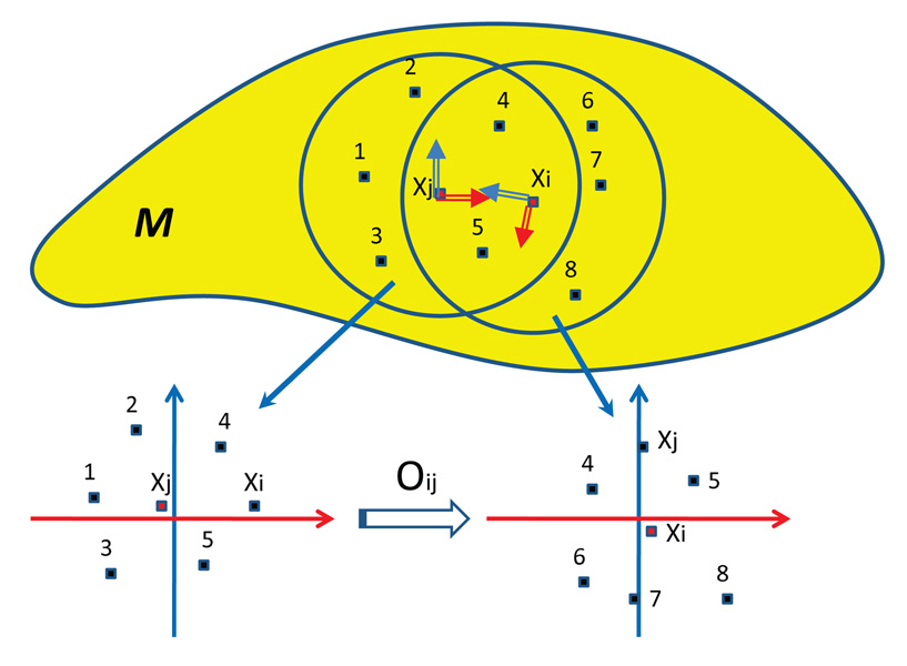
solves (2). The optimal orthogonal transformation O_ij can be either a rotation (i.e., an element of SO(d)), or a composition of a rotation and a reflection. Figure 1 is an illustration of this procedure.

Figure 1.

The orthonormal bases of the tangent planes T_xiℳ and T_xiℳ determined by local PCA are marked on top of the manifold by double arrows. The lower part demonstrates the projection of the data points onto the subspaces spanned by the orthonormal bases (the tangent planes). The coloring of the axes (blue and red) correspond to the coloring of the basis vectors. In this case, O_ij is a composition of a rotation and a reflection.

The determinant of O_ij classifies the two possible cases:

$$\text{det}{O}_{\mathit{\text{ij}}}=\{\begin{array}{cc}\hfill 1& \text{\hspace{1em}optimal transformation does not include a reflection},\hfill \\ \hfill -1& \text{\hspace{1em}optimal transformation includes a reflection}.\hfill \end{array}$$ (5)

We refer to the process of finding the optimal orthogonal transformation between bases as alignment. Note that not all bases are aligned; only the bases of nearby points are aligned. We set G = (V, E) to be the undirected graph with n vertices corresponding to the data points, where an edge between i and j exists iff their corresponding bases are aligned by the algorithm. We further encode the information about the reflections in a symmetric n × n matrix Z whose elements are given by

$$Z_{\mathit{\text{ij}}}=\{\begin{array}{cc}\hfill \text{det}{O}_{\mathit{\text{ij}}}\hfill & (i,j)\in E,\hfill \\ \hfill 0\hfill & (i,j)\notin E.\hfill \end{array}$$ (6)

That is, Z_ij = 1 if no reflection is needed, Z_ij = −1 if a reflection is needed, and Z_ij = 0 if the points are not nearby.

2.3. Synchronization

The third ingredient of the ODM algorithm is synchronization. If the manifold is orientable, then we can assign an orientation to each tangent space in a continuous way. For each x_i, the basis found by local PCA can either agree or disagree with that orientation. We may therefore assign a variable z_i ∈ {+1, −1} that designates if the PCA basis at x_i agrees with the orientation (z_i = 1) or not (z_i = −1). Clearly, for nearby points x_i and x_j whose bases are aligned, we must have that

$$z_i{z}_j^{-1}=z_{\mathit{\text{ij}}},(i,j)\in E.$$ (7)

That is, if no reflection was needed in the alignment stage (i.e., z_ij = 1), then either both PCA bases at x_i and x_j agree with the orientation (z_i = z_j = 1) or both disagree with the orientation (z_i = z_j = −1). Similarly, if a reflection was needed (z_ij = −1), then it must be the case that z_i = −z_j. In practice, however, we are not given an orientation for the manifold, so the values of the z_i’s are unknown. Instead, only the values of the z_ij’s are known to us after the alignment stage. Thus, we may try solving the system (7) to find the z_i’s. A solution exists iff the manifold is orientable. The solution is unique up to a global sign change, i.e., if (z₁, z₂, …, z_n) is a solution, then (−z₁, −z₂, …, −z_n) is also a solution. If all equations in (7) are accurate and the graph G is connected, then finding a solution can be obtained in a straightforward manner by simply traversing a spanning tree of the graph from the root to the leafs.

In practice, however, due to curvature effects and noise, some of the equations in (7) may be incorrect and we would like to find a solution that satisfies as many equations as possible. This maximum satisfiability problem is also known as the synchronization problem over the group ℤ₂ [15], and in [15, 7] we proposed spectral algorithms to approximate its solution. In [15] we used the top eigenvector (corresponding to the largest eigenvalue) of Z to find the solution, while in [7] we normalized the matrix Z and used the top eigenvector of that normalized matrix. Here we use the algorithm in [7], since we find the normalization to give much improved results.

Specifically, we normalize the matrix Z by dividing the elements of each row by the number of non-zero elements in that given row, that is,

$$𝒵=D^{-1}Z,$$ (8)

where D is a n × n diagonal matrix with $D_{\mathit{\text{ii}}}={\displaystyle {\sum }_{j=1}^n|z_{\mathit{\text{ij}}}|}$. In other words, D_ii = deg(i), where deg(i) is the degree of vertex i in the graph G. We refer to 𝒵 as the reflection matrix. Note that although 𝒵 is not necessarily symmetric, it is similar to the symmetric matrix D^−1/2Z D^−1/2 through

$$𝒵=D^{-1/2}(D^{-1/2}{\mathit{\text{Z D}}}^{-1/2})D^{1/2}.$$

Therefore, the matrix 𝒵 has n real eigenvalues ${\lambda }_1^{𝒵}>{\lambda }_2^{𝒵}\ge \cdots \ge {\lambda }_n^{𝒵}$ and n orthonormal eigenvectors ${\upsilon }_1^{𝒵},\dots ,{\upsilon }_n^{𝒵}$, satisfying

$$𝒵{\upsilon }_i^{𝒵}={\lambda }_i^{𝒵}{\upsilon }_i^{𝒵}.$$

We compute the top eigenvector ${\upsilon }_1^{𝒵}\in {ℝ}^n$ of 𝒵, which satisfies

$$𝒵{\upsilon }_1^{𝒵}={\lambda }_1^{𝒵}{\upsilon }_1^{𝒵},$$ (9)

and use it to obtain estimators ẑ₁, …, ẑ_n for the unknown variables z₁, …, z_n, in the following way:

$${\widehat{z}}_i=\text{sign}({\upsilon }_1^{𝒵}(i))=\frac{{\upsilon }_1^{𝒵}(i)}{|{\upsilon }_1^{𝒵}(i)|},i=1,2,\dots ,n.$$ (10)

The estimation by the top eigenvector is up to a global sign, since if ${\upsilon }_1^{𝒵}$ is the top eigenvector of 𝒵 then so is $-{\upsilon }_1^{𝒵}$ .

To see why (10) is a good estimator, we first analyze it under the assumption that the matrix Z contains no errors on the relative reflections. Denoting by ϒ the n × n diagonal matrix with ±1 on its diagonal representing the correct reflections z_i, i.e. ϒ_ii = z_i, we can write the matrix Z as

$$Z=\mathrm{\Upsilon }A{\mathrm{\Upsilon }}^{-1},$$ (11)

where A is the adjacency matrix of the graph G whose elements are given by

$$a_{\mathit{\text{ij}}}=\{\begin{array}{cc}1\hfill & (i,j)\in E,\hfill \\ 0\hfill & (i,j)\notin E,\hfill \end{array}$$ (12)

because in the error-free case $z_{\mathit{\text{ij}}}=z_i{z}_j^{-1}$ for (i, j) ∈ E. The reflection matrix 𝒵 can now be written as

$$𝒵=\mathrm{\Upsilon }(D^{-1}A){\mathrm{\Upsilon }}^{-1}.$$ (13)

Hence, 𝒵 and D⁻¹ A share the same eigenvalues. Since the normalized discrete graph Laplacian ℒ of the graph G is defined as

$$ℒ=I-D^{-1}A,$$ (14)

it follows that in the error-free case, the eigenvalues of I − 𝒵 are the same as the eigenvalues of ℒ. These eigenvalues are all non-negative, since ℒ is similar to the positive semidefinite matrix I − D^−1/2 AD^−1/2, whose non-negativity follows from the identity

$${\upsilon }^T(I-D^{-1/2}{\mathit{\text{AD}}}^{-1/2})\upsilon ={{\displaystyle \sum _{(i,j)\in E}\left(\frac{\upsilon (i)}{\sqrt{\text{deg}(i)}}-\frac{\upsilon (j)}{\sqrt{\text{deg}(j)}}\right)}}^2\ge 0,$$

for any υ ∈ ℝⁿ. In other words,

$$1-{\lambda }_i^{𝒵}={\lambda }_i^{ℒ}\ge 0,i=1,2,\dots ,n,$$ (15)

where the eigenvalues of ℒ are ordered in increasing order, i.e., ${\lambda }_1^{ℒ}\le {\lambda }_2^{ℒ}\le \cdots \le {\lambda }_n^{ℒ}$, and the corresponding eigenvectors ${\upsilon }_i^{ℒ}$ satisfy $ℒ{\upsilon }_i^{ℒ}={\lambda }_i^{ℒ}{\upsilon }_i^{ℒ}$. Furthermore, the sets of eigenvectors are related by

$${\upsilon }_i^{𝒵}=\mathrm{\Upsilon }{\upsilon }_i^{ℒ}.$$ (16)

If the graph G is connected, then the eigenvalue ${\lambda }_1^{ℒ}=0$ is simple and its corresponding eigenvector ${\upsilon }_1^{ℒ}$ is the all-ones vector 1 = (1, 1, …, 1)^T. Therefore,

$${\upsilon }_1^{𝒵}=\mathrm{\Upsilon }\mathbf{1},$$ (17)

and, in particular,

$${\upsilon }_1^{𝒵}(i)=z_i,i=1,2,\dots ,n.$$ (18)

This implies that in the error-free case, (10) perfectly recovers the reflections. In other words, the eigenvector ${\upsilon }_1^{𝒵}$ contains the orientation information of each tangent space. According to this orientation information, we can synchronize the orientations of all tangent spaces by flipping the orientation of the basis O_i whenever ${\upsilon }_1^{𝒵}(i)<0$. In conclusion, the above steps synchronize all the tangent spaces to agree on their orientations.

If the manifold is not orientable, then it is impossible to synchronize the orientation of the tangent spaces and the top eigenvector cannot be interpreted as before. We return to this interpretation later in the paper. For the moment, we just remark that the eigenvalues of A and Z (and similarly of ℒ and 𝒵) contain information about the number of orientation preserving and orientation reversing closed loops. To that end, consider first A^t(i, j), which is the number of paths of length t over the graph G that start at node i and end at node j. In particular, A^t(i, i) is the number of closed loops that start and end at node i. Therefore,

$$\text{Tr}(A^t)={\displaystyle \sum _{i=1}^n{A}^t(i,i)}={\displaystyle \sum _{i=1}^n{({\lambda }_i^A)}^t}$$

is the number of closed loops of length t. Similarly,

$$\text{Tr}(Z^t)={\displaystyle \sum _{i=1}^n{Z}^t(i,i)}={\displaystyle \sum _{i=1}^n{({\lambda }_i^Z)}^t}$$

is the number of orientation preserving closed loops minus the number of orientation reversing closed loops of length t. If the manifold is orientable then all closed loops are orientation preserving and the two traces are the same, but if the manifold is non-orientable then there are orientation reversing closed loops and therefore the eigenvalues of A and Z must differ.

If the manifold is determined to be orientable, then we can use the computed eigenvectors of 𝒵 for dimensionality reduction in the following manner. Specifically, we use point-wise multiplication of the eigenvectors of 𝒵 by the estimated reflections to produce new vectors υ̃₁, …, υ̃_n that are given by

$${\tilde{\upsilon }}_j(i)={\widehat{z}}_i{\upsilon }_j^{𝒵}(i),i,j=1,\dots ,n.$$ (19)

The relation (16) between the eigenvectors of 𝒵 and ℒ, and the particular form of the top eigenvector ${\upsilon }_1^{𝒵}$ given in (17) imply that the vectors υ̃₁, …, υ̃_n are eigenvectors of ℒ with ${\tilde{\upsilon }}_j={\upsilon }_j^{ℒ}$. The eigenvectors of ℒ are used in the diffusion map framework to embed the data points onto a lower dimensional Euclidean space, where distances between points approximate the diffusion distance [6]. Similarly, we can embed the data points using the following rule:

$$x_i\mapsto {\widehat{z}}_i({\lambda }_2^t{\upsilon }_2^{𝒵}(i),{\lambda }_3^t{\upsilon }_3^{𝒵}(i),\dots ,{\lambda }_k^t{\upsilon }_k^{𝒵}(i))\in {ℝ}^{k-1},$$ (20)

where t ≥ 0 is a parameter.

If the data points are sampled from the uniform distribution over the manifold, then the eigenvectors of the discrete graph Laplacian ℒ approximate the eigenfunctions of the Laplace-Beltrami operator [4], and it follows that the vectors υ̃_i that are used in our ODM embedding (20) also converge to the eigen-functions of the Laplace-Beltrami operator. If the sampling process is from a different distribution, then the υ̃_i’s approximate the eigenfunctions of the Fokker-Planck operator. By adapting the normalization rule suggested in [6] to our matrix Z, we can get an approximation of the eigenfunctions of the Laplace-Beltrami operator also for non-uniform distributions.

We remark that nothing prevents us from running the ODM algorithm in cases for which the sampling process from the manifold is noisy. We demonstrate the robustness of our algorithm through several numerical experiments in Section 4.

3. Orientable double covering

Every non-orientable manifold has an orientable double cover. Can we reconstruct the double covering from data points sampled only from the non-orientable manifold? In this section we give an affirmative answer to this question, by constructing a modified diffusion map embedding of the orientable double cover using only points that are sampled from the non-orientable manifold.

For simplicity of exposition, we start by making a simplifying assumption that we shall later relax. The assumption is that the orientable double cover has a symmetric isometric embedding in Euclidean space. That is, we assume that if ℳ is the non-orientable manifold, and ℳ̃ is its orientable double cover, then ℳ̃ has a symmetric isometric embedding in ℝ^q, for some q ≥ 1. Symmetric embedding means that for all x ∈ ℳ̃ ⊂ ℝ^q, also −x ∈ ℳ̃. This assumption is motivated by examples: the orientable double cover of the Möbius band is the cylinder, the orientable double cover of ℝP² is S² and the orientable double cover of the Klein bottle is T². The cylinder, S² and T² all have symmetric isometric embeddings in ℝ³ (q = 3). We believe that this assumption holds true in general, but its proof is beyond the scope of this paper³. Our assumption means that we have a ℤ₂ action on ℳ̃ given by x ↦ −x. We note that this ℤ₂ action is isometric and recall that if the group ℤ₂ is properly discontinuously acting on ℳ̃, then ℳ̃/ℤ₂ is non-orientable if and only if ℳ̃ has an orientation that is not preserved by the ℤ₂ action.

By our assumption, the orientable double covering ℳ̃ can be isometrically embedded into ℝ^q for some q so that ℤ₂x = −x for all x ∈ ℳ̃ and ℳ̃/ℤ₂ = ℳ. Denote the projection map as π : {x, −x} ⊂ ℳ̃ ↦ [x] ∈ ℳ. Under this assumption, each pair of antipodal points in ℳ̃ can be viewed as a single point in ℳ. In other words, for any point [x] ∈ ℳ, we can view it as two antipodal points x, −x ∈ ℳ̃ whose antipodal relationship is ignored.

We can now offer an interpretation of the matrix Z whose entries are given in (6). Recall that we have n data points in ℝ^p that are sampled from ℳ. We denote these points by [x₁], …, [x_n]. Associate to each [x_i] ∈ ℳ a point x_i ∈ ℳ̃ ⊂ ℝ^q such that π(x_i) = [x_i] and such that the entries of Z satisfy the following conditions: z_ij = 1 if x_j is in the ϵ-neighborhood of x_i; z_ij = −1 if x_j is the ϵ-neighborhood of ℤ₂x_i = −x_i; and z_ij = 0 if the distance between x_j and x_i and the distance between x_j and −x_i are both larger than ϵ. That is,

$$z_{\mathit{\text{ij}}}=\{\begin{array}{cc}\hfill 1& \text{if}{\Vert x_i-x_j\Vert }_{{ℝ}^q}<ϵ,\hfill \\ \hfill -1& \text{if}{\Vert x_i+x_j\Vert }_{{ℝ}^q}<ϵ,\hfill \\ \hfill 0& \text{otherwise}.\hfill \end{array}$$

Next, we build a 2n × 2n matrix Z̃ as follows:

$$\tilde{Z}≔\left[\begin{array}{cc}\hfill Z& \hfill -Z\\ \hfill -Z& \hfill Z\end{array}\right]=\left(\begin{array}{cc}\hfill 1& \hfill -1\\ \hfill -1& \hfill 1\end{array}\right)\otimes Z,$$ (21)

where ⊗ is the Kronecker product. The matrix Z̃ corresponds to 2n points over ℳ̃, while originally we had only n such points. We identify the additional points, denoted x_n+1, …, x_2n as x_n+i = −x_i for i = 1, …, n. With this identification, it is easily verified that the entries of $\tilde{Z}={({\tilde{z}}_{\mathit{\text{ij}}})}_{i,j=1}^{2n}$ are also given by

$${\tilde{z}}_{\mathit{\text{ij}}}=\{\begin{array}{cc}\hfill 1& \text{if}{\Vert x_i-x_j\Vert }_{{ℝ}^q}<ϵ,\hfill \\ \hfill -1& \text{if}{\Vert x_i+x_j\Vert }_{{ℝ}^q}<ϵ,\hfill \\ \hfill 0& \text{otherwise}.\hfill \end{array}$$

In a sense, the −Z in the (1, 2) and (2, 1) entries of Z̃ in (21) provides the lost information between π⁻¹([x_i]) and π−1([x_j]). We also define the matrices 𝒵̃ and ℒ̃ as

$$\widetilde{𝒵}=\left[\begin{array}{cc}\hfill 𝒵& \hfill -𝒵\\ \hfill -𝒵& \hfill 𝒵\end{array}\right]=\left(\begin{array}{cc}\hfill 1& \hfill -1\\ \hfill -1& \hfill 1\end{array}\right)\otimes 𝒵=\left(\begin{array}{cc}\hfill 1& \hfill -1\\ \hfill -1& \hfill 1\end{array}\right)\otimes D^{-1}Z,$$ (22)

and

$$\widetilde{ℒ}=\left[\begin{array}{cc}\hfill ℒ& \hfill -ℒ\\ \hfill -ℒ& \hfill ℒ\end{array}\right]=\left(\begin{array}{rr}\hfill 1& \hfill -1\\ \hfill -1& \hfill 1\end{array}\right)\otimes ℒ=\left(\begin{array}{rr}\hfill 1& \hfill -1\\ \hfill -1& \hfill 1\end{array}\right)\otimes (I-D^{-1}Z).$$ (23)

It is clear that the matrix 𝒵̃ is a discretization⁴ of the integral operator 𝒦̃_ϵ : L²(ℳ̃) → L²(ℳ̃), given by

$$({\widetilde{𝒦}}_{ϵ}f)(x)={\displaystyle {\int }_{\widetilde{ℳ}}{\tilde{K}}_{ϵ}(x,y)f(y)\mathit{\text{dy}},}$$ (24)

where the kernel function K̃_ϵ is given by

$${\tilde{K}}_{ϵ}(x,y)=\{\begin{array}{cc}\hfill \frac{1}{\text{vol}(B_{ϵ}(x)\cap \widetilde{ℳ})}\hfill & \text{if}{\Vert x-y\Vert }_{{ℝ}^q}<ϵ,\hfill \\ \hfill -\frac{1}{\text{vol}(B_{ϵ}(x)\cap \widetilde{ℳ})}\hfill & \text{if}{\Vert x+y\Vert }_{{ℝ}^q}<ϵ,,\hfill \\ \hfill 0\hfill & \text{otherwise},\hfill \end{array}$$ (25)

B_ϵ(x) is a ball of radius ϵ in ℝ^q centered at x, and the volume is measured using the metric of ℳ̃ induced from ℝ^q. Clearly, the integral operator 𝒦̃_ϵ commutes with the ℤ₂ action:

$${\widetilde{𝒦}}_{ϵ}{\mathbb{Z}}_{2}f={\mathbb{Z}}_2{\widetilde{𝒦}}_{ϵ}f,$$ (26)

where (ℤ₂f)(x) = f(−x). Moreover, the kernel of 𝒦̃_ϵ includes all “even” functions. That is, if f satisfies f(x) = f(−x) for all x ∈ ℳ̃, then 𝒦̃_ϵ f = 0. It follows that the eigenfunctions of 𝒦̃_ϵ with non-vanishing eigenvalues must be “odd” functions that satisfy f(x) = −f(−x).

Recall that the graph Laplacian ℒ converges to the Laplace-Beltrami operator in the limit n → ∞ and ϵ → 0 if the data points are sampled from the uniform distribution over the manifold. That is,

$$\underset{ϵ\to 0}{\text{lim}}\underset{n\to \mathrm{\infty }}{\text{lim}}\frac{1}{ϵ}ℒf(x)=m_2{\mathrm{\Delta }}_{ℳ}f(x),$$ (27)

where m₂ is a constant related to the second moment of the kernel function. Adapting this result to our case implies that we have the following convergence result for the matrix ℒ̃:

$$\underset{ϵ\to 0}{\text{lim}}\underset{n\to \mathrm{\infty }}{\text{lim}}\frac{1}{ϵ}(\widetilde{ℒ}f)(x)={\tilde{m}}_2[({\mathrm{\Delta }}_{\widetilde{ℳ}}f)(x)-({\mathrm{\Delta }}_{\widetilde{ℳ}}f)(-x)],$$ (28)

where m̃₂ is a constant. In other words, in the limit we recover the following operator:

$${\mathrm{\Delta }}_{\widetilde{ℳ}}-{\mathbb{Z}}_2{\mathrm{\Delta }}_{\widetilde{ℳ}}.$$ (29)

The Laplacian Δ_ℳ̃ also commutes with the ℤ₂ action, so by similar considerations, the kernel of Δ_ℳ̃ − ℤ₂ Δ_ℳ̃ contains all even functions, and the eigen-functions with non-zero eigenvalues are odd functions.

Suppose ϕ₁, ϕ₂, …, ϕ_2n and λ₁ ≥ λ₂ ≥ … ≥ λ_2n ≥ 0 are the eigenvectors and eigenvalues of ℒ̃. From the above discussion we have that λ_n+1 = … = λ_2n = 0 and ϕ₁, …, ϕ_n are odd vectors satisfying ϕ_l(i) = −ϕ_l(n+i) (1 ≤ l ≤ n). We define the map Φ̃_t for t > 0 as

$${\tilde{\mathrm{\Phi }}}_t:x_i\mapsto ({\lambda }_1^t{\varphi }_1(i),{\lambda }_2^t{\varphi }_2(i),\dots ,{\lambda }_n^t{\varphi }_n(i)),\text{\hspace{1em}for }i=1,2,\dots ,2n.$$ (30)

We refer to Φ̃_t as a modified diffusion map. Note that Φ̃_t uses only the odd eigenfunctions of the Laplacian over ℳ̃, whereas the classical diffusion map uses all eigenfunctions, both odd and even.

Our construction shows that from the information contained in the matrix Z, which is built solely from the non-orientable manifold ℳ, we obtain the odd eigenfunctions of the Laplacian over the double cover ℳ̃. The odd eigenfunctions are extremely useful for embedding the double cover. For example, the double cover of ℝP² is S² whose odd eigenfunctions are the odd degree spherical harmonics. In particular, the degree-1 spherical harmonics are the coordinate functions x, y and z (in ℝ³), so truncating the modified diffusion map Φ̃_t to ℝ³ results in an embedding of S² in ℝ³. Similarly, the first 3 eigenvectors of ℒ̃ (or equivalently, 𝒵̃) built up from the Klein bottle and the Möbius band allow us to get a torus and a cylinder, respectively. These reconstruction results are shown in Section 4.

We now return to the underlying assumption that the manifold ℳ̃ has a symmetric isometric embedding in ℝ^q for some q ≥ 1. While the assumption was useful to visualize the construction, we note that it is actually not necessary for the above derivation and interpretation. Indeed, the non-orientable manifold ℳ has an abstract orientable double cover ℳ̃ with ℤ₂ acting on it such that ℳ̃/ℤ₂ = ℳ. While the assumption allowed us to make a concrete specification of the ℤ₂ action (i.e., ℤ₂x = −x), this specification is not necessary in the abstract setup. The careful reader may check each and every step of the derivation and verify that they follow through also in the abstract sense. In particular, the matrix 𝒵̃ can be interpreted just as before, with x_n+i = ℤ₂x_i ∈ ℳ̃ for ℤ₂ being the abstract action. Moreover, the Laplacian over ℳ̃ still commutes with ℤ₂ and the matrix ℒ̃ converges to the operator given in (29). Thus, the modified diffusion mapping Φ̃_t given in (30) is an embedding of the abstract double cover. In the continuous setup, the eigenfunctions ${\{{\varphi }_n\}}_{n=1}^{\infty }$ of the operator Δ_ℳ̃ − ℤ₂Δ_ℳ̃ embed the abstract double cover ℳ̃ in the Hilbert space 𝓁₂ through the mapping

$$x\mapsto ({\lambda }_1^t{\varphi }_1(x),{\lambda }_2^t{\varphi }_2(x),\dots ,{\lambda }_n^t{\varphi }_n(x),\dots ),\text{\hspace{1em}for }x\in \widetilde{ℳ},$$ (31)

where

$$({\mathrm{\Delta }}_{\widetilde{ℳ}}-{\mathbb{Z}}_2{\mathrm{\Delta }}_{\widetilde{ℳ}}){\varphi }_n={\lambda }_n{\varphi }_n,n=1,2,\dots .$$

Finally, we show a useful “trick” to generate a point cloud over a non-orientable manifold without knowing any of the parametrizations that embed it in Euclidean space. For example, suppose we want to generate a point cloud over the Klein bottle, but we forgot its parametrization in ℝ⁴ (the parametrization is given later in (32)). There is still a rather simple way to proceed that only requires the knowledge of the orientable double cover. That is, given a non-orientable manifold ℳ from which we want to sample points in a Euclidean space, all we need to know is its orientable double cover ℳ̃ and its symmetric embedding in Euclidean space⁵. So, although we forgot the parametrization of the Klein bottle in ℝ⁴, we assume that we still remember that its double cover is T² and the parametrization of T² in ℝ³. From the symmetric embedding of T² in ℝ³, we now describe how to get a diffusion map embedding of the Klein bottle in Euclidean space. In general, from the symmetric embedding of ℳ̃ we describe how to get the diffusion map embedding of ℳ.

We start by sampling n points uniformly from ℳ̃ ∈ ℝ^q. Next, we double the number of points by setting x_n+i = −x_i for i = 1, …, n. We then build a 2n × 2n matrix $\tilde{A}={({\tilde{a}}_{\mathit{\text{ij}}})}_{i,j=1}^{2n}$ given by

$${\tilde{a}}_{\mathit{\text{ij}}}=\{\begin{array}{cc}\hfill 1\hfill & \text{if}{\Vert x_i-x_j\Vert }_{{ℝ}^q}<ϵ,\hfill \\ \hfill 1\hfill & \text{if}{\Vert x_i+x_j\Vert }_{{ℝ}^q}<ϵ,\hfill \\ \hfill 0\hfill & \text{otherwise}.\hfill \end{array}$$

We see that the matrix à does not distinguish between x and ℤ₂x, which leads to the previous identification {x, ℤ₂x} = [x] ∈ ℳ. After normalizing the matrix as before, it can be easily verified that it converges to an integral operator that has all the odd functions in its kernel and its non-zero eigenvalues correspond to even eigenfunctions. Moreover, in the limit of n → ∞ and ϵ → 0 we get convergence to the following operator:

$${\mathrm{\Delta }}_{\widetilde{ℳ}}+{\mathbb{Z}}_2{\mathrm{\Delta }}_{\widetilde{ℳ}}.$$

This means that the computed eigenvectors approximate the even eigenfunctions of the Laplacian over ℳ̃. That is, we compute eigenfunctions that satisfy ϕ_l(x) = ϕ_l(ℤ₂x) (for l = 1, …, n). As a result, these eigenfunctions are only functions of [x] and are the eigenfunctions of Δ_ℳ. Thus, the mapping

$$[x_i]\mapsto ({\lambda }_1^t{\varphi }_1(x_i),\dots ,{\lambda }_n^t{\varphi }_n(x_i)),\text{\hspace{1em}for }i=1,\dots ,n,$$

is the diffusion mapping of ℳ.

We remark that this construction can help us to build up more examples of non-orientable manifolds. For example, we can start from S^2d ⊂ ℝ^2d+1 and build up the diffusion map embedding of the non-orientable real projective space ℝP(2d) without knowing the parametrization of ℝP(2d).

4. Numerical examples

In this section we provide several numerical experiments demonstrating the application of ODM on simulative data. In our experiments, we measure the level of noise by the signal to noise ratio (SNR), which is defined in the following way. Suppose s₁, s₂, …, s_n ∈ ℝ^p is a set of “clean” data points that are located exactly on the manifold. This set of points is considered as the signal, and we define its sample variance as

$$\text{Var}(\text{Signal})=\frac{1}{\mathit{\text{np}}}{\displaystyle \sum _{i=1}^n{\Vert s_i-\mu \Vert }_{{ℝ}^p,}^2}$$

where $\mu =\frac{1}{n}{\displaystyle {\sum }_{i=1}^n{s}_i}$ is the sample mean. The set of noisy data points x₁, x₂, …, x_n are located off the manifold and are generated using the following process:

$$x_i=s_i+\sigma {\xi }_i,\text{\hspace{1em}for }i=1,\dots ,n,$$

where σ > 0 is a fixed parameter, and ξ ~ 𝒩 (0, I_p×p) are independently identically distributed (i.i.d.) standard multivariate normally distributed isotropic random variables. The SNR is measured in dB and is defined as

$$\text{SNR}[\text{dB}]=10{\text{log}}_{10}\frac{\text{Var}(\text{Signal})}{{\sigma }^2}.$$

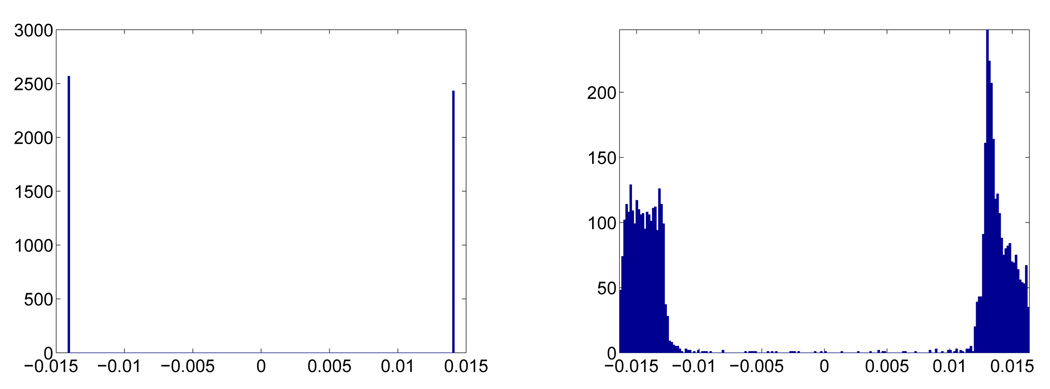
Our first example is the unit sphere S². This example demonstrates how to synchronize the orientation when the manifold is orientable. We sample n = 5000 points from S² uniformly without noise and run ODM with N = 100 nearest neighbors, and estimated the intrinsic dimension in the local PCA step using γ = 0.8. Then we sample another 5000 points from S² with SNR=5dB and run ODM with the same parameters. In both cases, the intrinsic dimension is estimated correctly as d̂ = 2. The histograms of the top eigenvector ${\upsilon }_1^{𝒵}$ of both cases are shown in Figure 2. The results show the robustness of ODM in orientation synchronization.

Figure 2.

Histogram of the values of the top eigenvector ${\upsilon }_1^{𝒵}$. Left: clean S²; Right: S² contaminated by 5dB noise. Note that the eigenvector is normalized so its values concentrate around ± $\frac{1}{\sqrt{n}}$ instead of ±1.

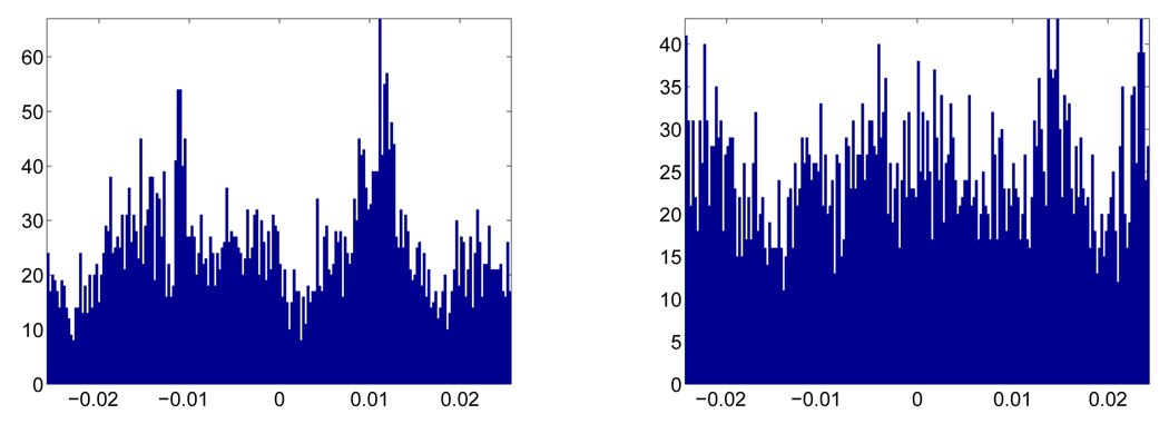
Next we show how the ODM algorithm helps us to determine if a given manifold is orientable or not. We sample 5000 points from the Klein bottle embedded in ℝ⁴ and ℝP(2) embedded in ℝ⁴ without noise, respectively. Then run the ODM algorithm for these two data sets with N = 200 and γ = 0.8. The histograms of the top eigenvectors are shown in Figure 3. It shows that when the underlying manifold is non-orientable, the values of the first eigenvector of the ODM do not cluster around two distinguished positive and negative values.

Figure 3.

Histogram of the values of the top eigenvector ${\upsilon }_1^{𝒵}$. Left: Klein bottle; Right: ℝP².

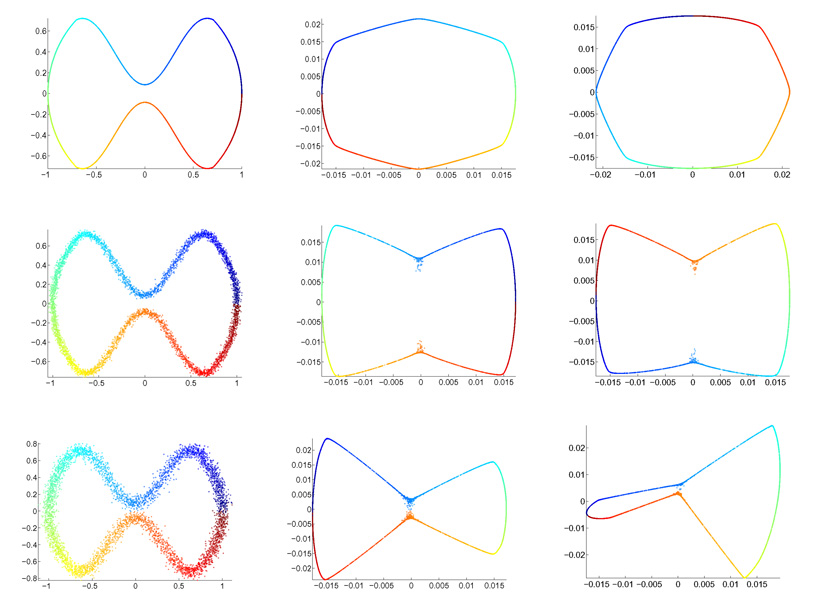
We proceed to considering the application of ODM for dimensionality reduction, looking at data points sampled from the bell-shaped, closed, non-intersected curve, which is parameterized by C(θ) = (x(θ), y(θ)), θ ∈ [0, 2π], where

$$\begin{array}{c}x(\theta )=\text{cos}(\theta ),\hfill \\ y(\theta )=\{\begin{array}{cc}\text{sin}(\theta )\hfill & \text{for}\theta \in [0,\pi /4]\cup [3\pi /4,5\pi /4]\cup [7\pi /4,2\pi ],\hfill \\ \text{sin}(\theta )\left(1-e^{-{(2\theta -\pi )}^2}+e^{-{(\pi /2)}^2}\right)\hfill & \text{otherwise}.\hfill \end{array}\hfill \end{array}$$

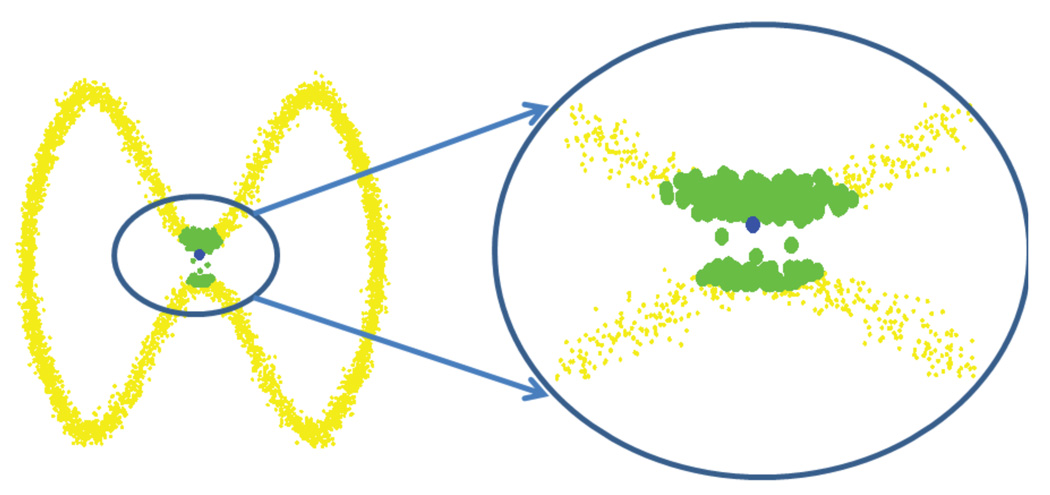
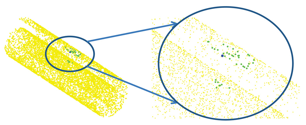
The curve is depicted in Figures 4 and 5. Note that the isthmus of C(θ) $(\text{near }\theta =\frac{\pi }{2}\text{ and }\theta =\frac{3\pi }{2})$ imposes a difficultly whenever the noise is too large or the sampling rate is too low. This difficulty is due to the identity of the nearest neighbors, as illustrated in Figure 4. It reflects the fact that the nearest neighbors are neighbors in the extrinsic sense (when the distance is measured by the Euclidean distance), but not in the intrinsic sense (when the distance is measured by the geodesic distance). To cope with this difficulty, we first cluster the nearest neighbors in order to find the “true” neighbors in the geodesic distance sense, prior to applying PCA. For clustering the points in 𝒩_xi we apply the spectral clustering algorithm [13], and for PCA we consider only the points that belong to the cluster of x_i.

Figure 4.

The bell shaped curve: the green points are the nearest neighbors of the blue point. The SNR is 30dB.

Figure 5.

From left to right: the input data set consisting of n = 5000 points, embedding by diffusion map, and embedding by ODM. Both the data set and the embeddings are colored by the parameter θ. The rows from top to bottom correspond to clean data, SNR=30dB and SNR=24dB.

We applied ODM to 5000 points from C(θ) without noise, with parameters N = 200 and γ = 0.8, and then embed the data points into ℝ² using the second and third eigenvectors and (20). We repeat the same steps for noisy data sets with SNR=30dB and SNR=24dB. Figure 5 shows the original data set, the diffusion map (DM) embedding, and the ODM embedding. In the DM algorithm, we used the Gaussian kernel exp{−‖x_i − x_j‖²/σ} with σ = 0.5. As expected, the embedding results of ODM and DM are comparable.

Our next example is the Swiss roll, a manifold often used by machine learners as a testbed for dimensionality reduction methods. The Swiss roll model is the following manifold S embedded in ℝ³:

$$\begin{array}{c}x(t,s)=\frac{3\pi (1+2t)}{8}\text{cos}\frac{3\pi (1+2t)}{2},\hfill \\ y(t,s)=s,\hfill \\ z(t,s)=\frac{3\pi (1+2t)}{8}\text{sin}\frac{3\pi (1+2t)}{2},\hfill \end{array}$$

for (t, s) ∈ [0, 1] × [0, 21]. The Swiss roll model exhibits the same difficulty we encountered before with the bell-shape curve, namely, that the geodesically distant points might be close in the Euclidean sense (see Figure 6). Moreover, unlike the manifolds considered before, the Swiss roll has a boundary. To cope with these problems, we again apply the spectral clustering algorithm [13] prior to the local PCA step of the ODM algorithm.

Figure 6.

The Swiss roll: the yellow points are the original data, while the green points are nearest neighbors of the blue point. The points are sampled from the Swiss roll without any noise.

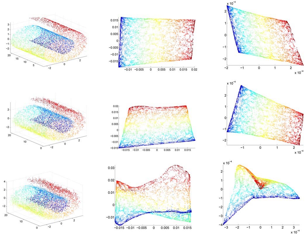
We sampled n = 7000 points from the Swiss roll without noise, run ODM with parameters N = 40 and γ = 0.8, and then embedded the data points into ℝ² by the second and third eigenvectors using (20). We repeated the same steps for data sets with SNR values 50dB, 30dB and 25dB. Figure 7 shows the original data, the embedding by DM, and the embedding by ODM. In the DM algorithm, we used the Gaussian kernel with σ = 5.

Figure 7.

From left to right: the input data, the embedding by diffusion map, and the embedding by ODM. The data sets and the embeddings are colored by the parameter t. From top to bottom: clean data set, SNR=30dB and SNR=25dB.

In conclusion, we see that besides determining the orientability of the manifold, ODM can also be used as a dimensionality reduction method.

In the last part of this section we demonstrate results about recovering the orientable double covering of a non-orientable manifold as discussed in Section 3. First we demonstrate the orientable double covering of ℝP(2), Klein bottle and Möbius band in Figure 8. For ℝP(2), we use the following embedding inside ℝ⁴:

$$(x,y,z)\mapsto (\mathit{\text{xy}},\mathit{\text{xz}},y^2-z^2,2\mathit{\text{yz}})$$

where (x, y, z) ∈ S² ⊂ ℝ³. We sample 8000 points uniformly from S² and map the sampling points to ℝP(2) by the embedding, which gives us a non-uniform sampling data set. Then we evaluate eigenvectors of the 16000 × 16000 sparse matrix 𝒵̃ constructed from the data set with N = 40 and get the approximation of the coordinates of the orientable double covering which allows us to get the orientable double covering (Figure 8, left panel).

Figure 8.

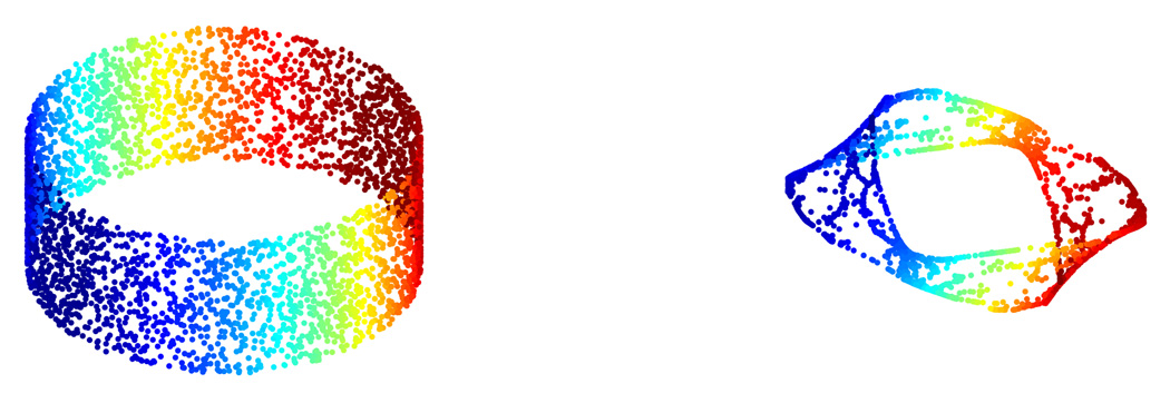
Left: the orientable double covering of ℝP(2), which is S²; Middle: the orientable double covering of the Klein bottle, which is T²; Right: the orientable double covering of the Möbius strip, which is a cylinder.

For the Klein bottle, we apply the following embedding inside ℝ⁴:

$$\{\begin{array}{c}x=(2\text{ cos }\upsilon +1)\text{ cos }u\hfill \\ y=(2\text{ cos }\upsilon +1)\text{ sin }u\hfill \\ z=2\text{ sin }\upsilon \text{cos}(u/2)\hfill \\ w=2\text{ sin }\upsilon \text{sin}(u/2)\hfill \end{array}$$ (32)

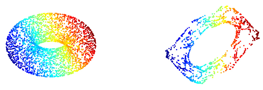
where (u, υ) ∈ [0, 2π] × [0, 2π]. We sample 8000 points uniformly from [0, 2π] × [0, 2π] and map the sampling points to the Klein bottle by the embedding, which gives us a non-uniform sampling data set over the Klein bottle. Then we run the same procedure as in ℝP(2) with N = 40 and get the result (Figure 8, middle panel).

For the Möbius band, we use the following parametrization:

$$\{\begin{array}{c}x=(a+b\upsilon \text{ cos}(0.5u))\text{ cos}(u)\hfill \\ y=(a+b\upsilon \text{ cos}(0.5u))\text{ sin}(u)\hfill \\ z=b\upsilon \text{ sin}(0.5u)\hfill \end{array}$$

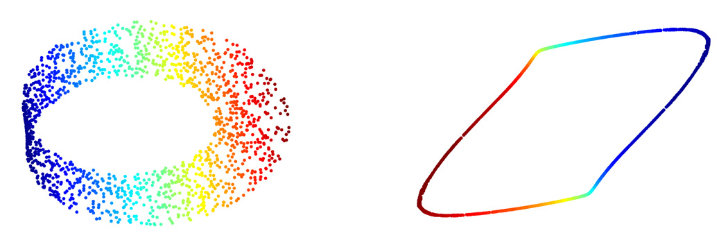
where a = 3, b = 5 and (u, υ) ∈ [−1, 1]×[0, 2π]. As above, we sample 8000 points uniformly from [−1, 1]×[0, 2π] and map the sampling points to the Möbius band by the parametrization, which gives us a non-uniform sampling data set. Then we run the same procedure with N = 20 and get the result (Figure 8, right panel). It is worth mentioning that when b is small, e.g., b = 1, we fail to recover the cylinder, as can be seen in Figure 9. This difficulty comes from the lack of information in the width of the band when b is too small.

Figure 9.

Left: the Möbius band embedded in ℝ³ with b = 1; Right: the algorithm failed to recover the cylinder.

Last, we demonstrate how to get a non-orientable manifold by constructing the 𝒜̃ matrix as discussed in Section 3. We start from showing the spectrum of ℝP(2) constructed by gluing the antipodal points of S² together. We build up 𝒜̃ by taking N = 50 from 16000 data points sampled from S² embedded in ℝ³:

$$\{\begin{array}{c}x=\text{sin}(\theta )\text{ cos}(\varphi )\hfill \\ y=\text{sin}(\theta )\text{ sin}(\varphi )\hfill \\ z=\text{cos}(\theta )\hfill \end{array}$$

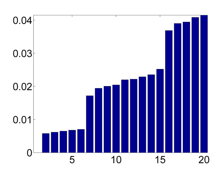
which is the approximation of the Laplace-Beltrami operator over S²/ℤ₂ ≅ ℝP(2). The spectrum of the operator is shown in Figure 10.

Figure 10.

Bar plot of the eigenvalues of the graph Laplacian of the abstract ℝP(2) constructed from gluing antipodal points of S². The multiplicities 1, 5, 9, … correspond to the even degree spherical harmonics.

Then we demonstrate the reconstruction of the orientable double covering of an abstract non-orientable manifold, by which we mean an abstract non-orientable manifold not yet embedded inside any Euclidean space. We start from sampling 16000 points from a cylinder C embedded in ℝ³, which is parameterized by:

$$\{\begin{array}{c}x=2\text{ cos }\theta \hfill \\ y=2\text{ sin }\theta \hfill \\ z=a\hfill \end{array}$$

where (θ, a) ∈ [0, 2π]×[−2, 2], and run the following steps. First we fix N = 50, and build up 𝒜̃, the approximation of the Laplace-Beltrami operator over C/ℤ₂ by gluing the antipodal points together. Note that C/ℤ₂ is an abstract Möbius band up to now. Second, we embed C/ℤ₂ by applying diffusion map, where we take the second to fifth eigenvectors of 𝒜̃, that is, we embed C/ℤ₂ into ℝ⁴. Finally we run ODM with N = 50 over the embedded C/ℤ₂ to reconstruct the double covering. The result, shown in Figure 11, shows that we recover back a cylinder. Similarly, we run the same process with the same parameters N = 50 and the second to fifth eigenvectors of 𝒜̃ to embed T²/ℤ₂ and S²/ℤ₂ into ℝ⁴, and then run ODM with N = 50, which results in the reconstruction of the orientable double covering of an abstract Klein bottle and ℝP(2). The results are shown in Figure 12 and 13. Using different number of eigenvectors for embedding, for example, from the second to sixth or from the second to seventh eigenvectors give us similar results.

Figure 11.

Left: the cylinder embedded in ℝ³; Right: the recovered cylinder.

Figure 12.

Left: the torus embedded in ℝ³; Right: the recovered torus.

Figure 13.

Left: S² embedded in ℝ³; Right: the recovered S².

Note that in the above three examples shown in Figures 11, 12 and 13, the recovered objects look different from the original one. This distortion mainly comes from the following step: the embedding by diffusion map chosen in the demonstration is not isometric but just an approximation of an isometric embedding.

5. Summary and Discussion

We introduced an algorithm for determining the orientability of a manifold from scattered data. If the manifold is orientable then the algorithm synchronizes the orientations and can further be used for dimensionality reduction in a similar fashion to the diffusion map framework.

The algorithm consists of three steps: local PCA, alignment and synchronization. In the synchronization step we construct a matrix 𝒵, which for an orientable manifold is shown to be similar to the normalized Laplacian ℒ. For non-orientable manifolds this similarity does not hold anymore and we show how to obtain an embedding of the orientable double covering using the eigenvectors of the Kronecker product $\widetilde{𝒵}=\left(\begin{array}{cc}\hfill 1& \hfill -1\\ \hfill -1& \hfill 1\end{array}\right)\otimes 𝒵$. In particular, we show that the eigenvectors of 𝒵̃ approximate the odd eigenfunctions of the Laplacian over the double covering. We also show how to using this observation in order to embed an abstract non-orientable manifold in Euclidean space given its orientable double covering.

We comment that the reflection matrix 𝒵 can also be built by taking a kernel function into consideration, like the weighted graph Laplacians discussed in [6].

For example, we may replace the definition (6) of Z by

$$Z_{\mathit{\text{ij}}}=\{\begin{array}{cc}\hfill e^{-}\frac{{\Vert x_i-x_j\Vert }^2}{\sigma }\text{det}{O}_{\mathit{\text{ij}}}\hfill & (i,j)\in E,\hfill \\ \hfill 0\hfill & (i,j)\notin E.\hfill \end{array}$$ (33)

and

$$𝒵=D^{-1}Z,$$ (34)

where D is a n × n diagonal matrix with $D_{\mathit{\text{ii}}}={\displaystyle {\sum }_{j=1}^n|z_{\mathit{\text{ij}}}|}$. All the results in this paper also apply to this kernelized reflection matrix.

One possible application of our framework is the geometrical and topological study of high contrast local patches that are extracted from natural images [10]. Computational topology methods were used in [5] to conclude that this data set has the topology of the Klein bottle. This result may perhaps be confirmed using the methods presented here.

Finally, we remark that while the reflection matrix only uses the information in det O_ij, it seems natural also to take into account all the information in O_ij. This modification will be the subject of a separate publication.

References

- 1.Arun KS, Huang TS, Blostein SD. Least-squares fitting of two 3-D point sets. IEEE Trans. Patt. Anal. Mach. Intell. 1987;9(5):698–700. doi: 10.1109/tpami.1987.4767965. [DOI] [PubMed] [Google Scholar]
- 2.Belkin M, Niyogi P. Laplacian eigenmaps for dimensionality reduction and data representation. Neural Computation. 2003;15(6):1373–1396. [Google Scholar]
- 3.Belkin M, Niyogi P. Towards a theoretical foundation for Laplacian-based manifold methods. Proceedings of the 18th Conference on Learning Theory (COLT); 2005. pp. 486–500. [Google Scholar]
- 4.Belkin M, Niyogi P. Advances in Neural Information Processing Systems (NIPS) MIT Press; 2007. Convergence of Laplacian eigenmaps. [Google Scholar]
- 5.Carlsson G, Ishkhanov T, de Silva V, Zomorodian A. On the local behavior of spaces of natural images. International Journal of Computer Vision. 2008;76(1):1–12. [Google Scholar]
- 6.Coifman RR, Lafon S. Diffusion maps. Applied and Computational Harmonic Analysis. 2006;21(1):5–30. [Google Scholar]
- 7.Cucuringu M, Lipman Y, Singer A. Sensor network localization by eigenvector synchronization over the Euclidean group. doi: 10.1145/2240092.2240093. Submitted for publication. [DOI] [PMC free article] [PubMed] [Google Scholar]
- 8.Donoho DL, Grimes C. Hessian eigenmaps: Locally linear embedding techniques for high-dimensional data. Proceedings of the National Academy of Sciences of the United States of America. 2003;100(10):5591–5596. doi: 10.1073/pnas.1031596100. [DOI] [PMC free article] [PubMed] [Google Scholar]
- 9.Hein M, Audibert J, von Luxburg U. From graphs to manifolds - weak and strong pointwise consistency of graph Laplacians. Proceedings of the 18th Conference on Learning Theory (COLT); 2005. pp. 470–485. [Google Scholar]
- 10.Lee AB, Pedersen KS, Mumford D. The non-linear statistics of high-contrast patches in natural images. International Journal of Computer Vision. 2003;54(13):83–103. [Google Scholar]
- 11.Little AV, Lee J, Jung YM, Maggioni M. Estimation of intrinsic dimensionality of samples from noisy low-dimensional manifolds in high dimensions with multiscale SVD. 2009 IEEE/SP 15th Workshop on Statistical Signal Processing; 2009. pp. 85–88. [Google Scholar]
- 12.Nadler B, Lafon S, Coifman RR, Kevrekidis IG. Diffusion maps, spectral clustering and reaction coordinates of dynamical systems. Applied and Computational Harmonic Analysis. 2006;21(1):113–127. [Google Scholar]
- 13.Ng AY, Jordan MI, Weiss Y. On spectral clustering: Analysis and an algorithm. In: Leen TK, Dietterich TG, Tresp V, editors. Advances in neural information processing systems 14. Cambridge, MA: MIT Press; 2002. [Google Scholar]
- 14.Roweis ST, Saul LK. Nonlinear dimensionality reduction by locally linear embedding. Science. 2000;290(5500):2323–2326. doi: 10.1126/science.290.5500.2323. [DOI] [PubMed] [Google Scholar]
- 15.Singer A. Angular synchronization by eigenvectors and semidefinite programming. doi: 10.1016/j.acha.2010.02.001. In press. [DOI] [PMC free article] [PubMed] [Google Scholar]
- 16.Singer A. From graph to manifold Laplacian: The convergence rate. Applied and Computational Harmonic Analysis. 2006;21(1):128–134. [Google Scholar]
- 17.Tenenbaum JB, de Silva V, Langford JC. A Global Geometric Framework for Nonlinear Dimensionality Reduction. Science. 2000;290(5500):2319–2323. doi: 10.1126/science.290.5500.2319. [DOI] [PubMed] [Google Scholar]