Functional connectivity in slow-wave sleep: identification of synchronous cortical activity during wakefulness and sleep using time series analysis of electroencephalographic data

SUMMARY

Sleep is a behavioral state ideal for studying functional connectivity because it minimizes many sources of between-subject variability that confound waking analyses. This is particularly important for potential connectivity studies in mental illness where cognitive ability, internal milieu and active psychotic symptoms can vary widely across subjects. We, therefore, sought to adapt techniques applied to magnetoencephalography for use in high-density electroencephalography (EEG), the gold-standard in brain-recording methods during sleep. Autoregressive integrative moving average modeling was used to reduce spurious correlations between recording sites (electrodes) in order to identify functional networks. We hypothesized that identified network characteristics would be similar to those found with magnetoencephalography, and would demonstrate sleep stage-related differences in a control population. We analysed 60-s segments of low-artifact data from seven healthy human subjects during wakefulness and sleep. EEG analysis of eyes-closed wakefulness revealed widespread nearest-neighbor positive synchronous interactions, similar to magnetoencephalography, though less consistent across subjects. Rapid eye movement sleep demonstrated positive synchronous interactions akin to wakefulness but weaker. Slow-wave sleep (SWS), instead, showed strong positive interactions in a large left fronto-temporal-parietal cluster markedly more consistent across subjects. Comparison of connectivity from early SWS to SWS from a later sleep cycle indicated sleep-related reduction in connectivity in this region. The consistency of functional connectivity during SWS within and across subjects suggests this may be a promising technique for comparing functional connectivity between mental illness and health.

INTRODUCTION

The field of functional neuroimaging has increasingly focused on the study of interactions among brain regions. While considerable information has been gained through identification and localization of functionally specific cortical areas, a growing body of work suggests that the emergence of behavior and cognition are dependent upon the existence and integrity of dynamic neuronal networks, which are conserved across individuals. These studies of functional connectivity have been performed primarily using functional magnetic resonance imaging (fMRI), correlating the blood oxygen level-dependent signal either during task-specific activities or during resting states. Task-negative networks, also known as resting state or the ‘default mode network’, appear to involve posterior cingulate cortex, medial prefrontal cortex, inferior temporal cortex and parahippocampal gyrus, as well as lateral parietal cortex (see Bullmore and Sporns, 2009; Damoiseaux and Grecius, 2009 for recent reviews of the functional connectivity literature). Methods have also been developed to assess dynamic synchronous interactions among brain regions using magnetoencephalography (Langheim et al., 2006; Leuthold et al., 2005). However, none of these methods is suitable for studies during sleep due to required radiation exposure [positron emission tomography (PET)], or difficulty achieving sleep due to scanner noise (fMRI) or discomfort [fMRI and magnetoencephalography (MEG)].

It has been demonstrated that autocorrelation structure inherent to time series data risks the identification of spurious cortical interactions, and that these confounds may be addressed prior to correlation analysis through the use of Box–Jenkins autoregressive integrative moving average (ARIMA) modeling (Box and Jenkins, 1970; Leuthold et al., 2005). Focusing on synchronous correlations, stable dynamic networks were revealed with considerable similarity across subjects (Langheim et al., 2006).

Expanding on this previous work, we used ARIMA modeling to analyse high-density electroencephalographic (HD-EEG) data obtained during overnight sleep studies. The benefit of HD-EEG over MEG resides in the capacity for more ambulatory data collection, allowing for longer recording sessions and greater behavioral variability, such as full body motion and sleep. While concerns regarding signal blurring exist with EEG, the use of HD-EEG and the development of data analysis methods serve to minimize this (Michel et al., 2004). As a result, the millisecond temporal resolution of MEG is accessible through HD-EEG. A secondary benefit to use of HD-EEG is the lower expense of purchasing and maintaining the equipment, opening this field of inquiry to more laboratories and larger study populations with the prospect of greater clinical applicability.

Sleep was chosen as a behavioral state as it represents a great equalizer across study subjects. Slow-wave sleep (SWS) and rapid eye movement (REM) sleep are not dependent upon participant effort, skill or intellectual capacity, and require little more than willingness to undergo overnight polysomnography. Conversely, when functional connectivity is studied during behavioral tasks, their control conditions, or resting wakeful states in which attention and the internal milieu is not directly focused, significant confounds are introduced. These features make the study of sleep ideal for future longitudinal studies and work with mentally ill populations in whom functional connectivity is speculated to be aberrant.

As a preliminary step, we sought to determine the feasibility of using HD-EEG to compare network connectivity identified during eyes-closed wakefulness to that identified for SWS and REM stages, anticipating differences in functional connectivity among these behavioral states. We felt that comparison of three distinct behavioral states would reveal notable differences in connectivity, and should therefore be undertaken prior to exploring changes within any one of these states. We hypothesized that synchronous networks identified with this methodology in a restful waking state would be grossly similar to those identified with magnetoencephalography. At the same time, we expected that connectivity in sleep stages would demonstrate differences from waking data.

Specific challenges to accomplishing these goals with HD-EEG include the existence of autocorrelation structure within the HD-EEG signals themselves, as well as the potential overlap between spatial blurring (resulting from volume currents passing through various tissue types on their way to scalp electrodes) and functional connectivity. To illustrate autocorrelation influences, consider the redundant information present in the slope and upper and lower limits of time series fluctuations. The predictability imparted from that structure represents redundant information, which, in turn, exaggerates correlation. ARIMA modeling was developed to limit this by minimizing autocorrelation and partial autocorrelation structure. While the influence of blurred signals may be reduced through ARIMA modeling, the use of partial cross-correlation (PCC) analysis further minimizes broad cortical oscillations (whether from strong signals or from spatial blurring) from influencing encephalographic measures of functional connectivity. Although some potentially relevant brain signal may be reduced (for instance, some brainstem signal modulating the entire cortex simultaneously), what is left are more localized interactions. While the potential loss of information may reduce estimates of functional connectivity, it does so in a trade-off against identification of spurious correlations.

Therefore, to accomplish the goals of identifying functional connectivity with HD-EEG while showing variation in this connectivity with wakefulness and sleep stages, we identified the structure of HD-EEG time series by fitting appropriate ARIMA components. We then used the model obtained to derive prewhitened residuals of the series (time series close to stationary white noise devoid of predictable structure). The residuals were then used to estimate pairwise interactions between series using PCC. The resultant synchronous networks characterized during quiet wakefulness were compared with those obtained during REM and SWS.

MATERIALS AND METHODS

Subjects and recordings

HD-EEG was recorded in seven healthy subjects (one woman and six men, mean age 38.6 ± 7.7 years, range 29–54 years). Written informed consent was obtained from each subject following a screening for medical and psychiatric illness. The study was approved by the University of Wisconsin Institutional Review Board. Data were collected using a 256-channel Electrical Geodesics Hydrocel sensor net (Eugene, OR, USA). This net employed spongeless electrodes filled with conductive gel to improve skin contact and stability of the net during the recording. Participants were allowed to sleep at their self-reported bedtime. Fig. 1 displays a two-dimensional projection of the 256-channel array. Data were collected at 500 Hz (0.1 Hz highpass filter and 200 Hz lowpass filter amplifier settings) during overnight polysomnography. Electrooculogram and electromyogram (EMG) channels were derived from the 256-channel net to aid in sleep scoring. Sleep stages were visually scored for 20-s epochs on the EEG referenced to the mastoid (C3A2 and C4A1 derivations). In order to maintain channel to channel numerical relationships, all channels were included in the data analysis despite noise or high impedance, as those characteristics precluded significant correlations between those and other channels. Time series of eyes-closed wakefulness preceding sleep onset, as well as scored sleep stages, were visually inspected for artifacts. Sixty-second segments of low-artifact data were isolated from five different behavioral states: eyes-closed wakefulness; early SWS; late SWS; REM with low to absent rapid eye movements; and REM with high numbers of rapid eye movements.

Figure 1.

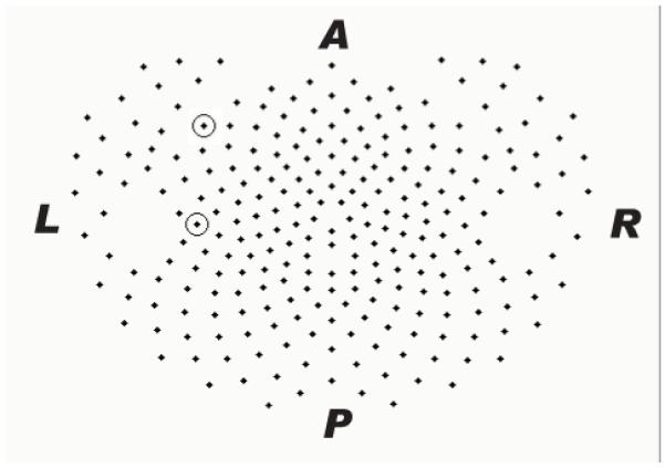
Two-dimensional projection of the 256 sensor Electrical Geodesics Hydrocel layout. Encircled sensors are #54 (more anterior) and #70 for which data are illustrated in Figures. 2, 3, and 4. L= left, R= right, A= anterior, and P= posterior.

Data analysis

A specific goal for this study was to assess the interactions between time series in pairs of sensors. To that end, individual series must be stationary, as non-stationarities in the time series may lead to spurious correlations (Box and Jenkins, 1970; Priestley, 1981). Our analyses began with modeling the individual time series to derive relatively stationary residuals, which could then be used to compute pairwise correlations. Box–Jenkins ARIMA modeling analyses were performed using SPSS (SPSS for Windows, version 10.1.0, SPSS, Chicago, IL, USA), and repeated using software written in Matlab (The MathWorks™ Novi, MI, USA). Autocorrelation (ACF) and partial autocorrelation (PACF) functions were plotted for 25 lags, corresponding to 50 ms given our sampling rate.

The goal of ARIMA modeling in the context of HD-EEG studies in functional connectivity is to minimize the influence of signal autocorrelation and spatial blurring on correlation measures between sensor time series. This is accomplished by removing identifiable and predictable structure from each time series (Leuthold et al., 2005; Langheim et al., 2006). Predictable structure may be identified through graphing of ACF and PACF. Analysis of ACFs and PACFs for individual channels demonstrated a need for first-order differencing (subtraction of time point n − 1 from time point n), which was applied to all data series as an initial processing step. Subsequent inspection of ACFs and PACFs of the differenced series indicated the presence of autoregressive (AR) and moving average (MA) components. Extensive model fitting and post-processing analyses were performed on a subset of subjects and channels using programs written for the purpose within Matlab. The number of significant autocorrelations and partial autocorrelations were minimized over multiple subjects and multiple sensor data sets within subjects, using from 0 to 50 AR orders in exhaustive combination with 0 to 20 MA orders, and 0 or 1 order of differencing. For each of these combinations, autocorrelograms and partial autocorrelograms were examined, and a nadir was identified among remaining significant time lags from 1 to 25 (Leuthold et al., 2005; Langheim et al., 2006). Through this evaluation, the optimal model resulting in quasi-stationarity of residual time series for the majority of data analysed consisted of 40 AR orders (AR = 40) and one MA order (MA = 1), in addition to the aforementioned first order differencing (I = 1). After prewhitening of each individual time series using the 40,1,1 ARIMA model, individual pairwise interactions between sensors were calculated using PCC analysis, taking into account all other pairwise interactions among all other sensors. Plots of these pairwise interactions were made, demonstrating positive PCCs in green and negative PCCs in red, using thresholds both of significance corrected for multiple comparisons and absolute value of the PCC.

RESULTS

ARIMA modeling of HD-EEG data

A total of 8960 time series of 60-s duration were available for analysis (seven subjects by 256 by five time series each). The results of ARIMA modeling are demonstrated with an illustrative sensor (#70) in Figs 2 and 3. Fig. 2 shows 6 s of raw data, the same data following first order differencing, and the residual time series after application of the (40,1,1) ARIMA model for channel #70. While the raw series was non-stationary with respect to its mean and variance (as evidenced by the great deal of structured variability), this non-stationarity was considerably reduced after differencing, and further eliminated through ARIMA modeling. In order to underscore this non-stationarity, Fig. 3 shows ACFs (upper panels) and PACFs (lower panels) for the same data shown in Fig. 2. The ACFs and PACFs show non-stationarity in the raw data (demonstrable by the highly significant values at multiple time lags), and show that this non-stationarity was considerably reduced but not eliminated following differencing. ARIMA modeling further reduces the degree of non-stationarity, as the number of significant values across time lags approaches the standard error. Results were similar in other sensors within the same subject as well as across all subjects in wakefulness, REM and SWS.

Figure 2.

Data from sensor #70 (see Figure 1) before and after differencing and full ARIMA modeling (refer to the text for details). These data are from a 6 second portion of a total 60 seconds analyzed.

Figure 3.

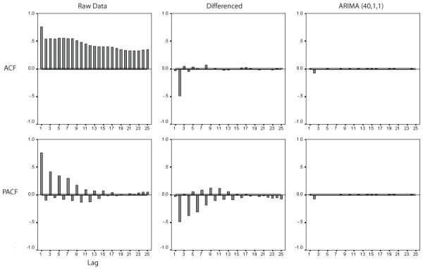
Autocorrelation functions (ACF) and partial autocorrelation functions (PACF) for the same subject and sensor as in Figure 2, before and after differencing and ARIMA modeling (refer to the text for details).

Cross-correlation analysis

Fig. 4 demonstrates the importance of prewhitening time series before accurate estimates of cross-correlation values may be calculated. At the far left, the cross-correlation function (CCF) between two sensor time series of raw data is plotted. The graph consists of large, highly statistically significant correlation values throughout the entirety of ± 50 ms lag. Differencing alone of the time series prior to cross-correlation calculation, as demonstrated by the middle graph, reveals a confounding oscillatory function, which achieves statistical significance across time lags. In contrast, the CCF computed using the prewhitened series of residuals following (40,1,1) ARIMA modeling consists of significant interaction within a focused temporal window of less than 10 ms. It can be seen that, although smaller, these values extend beyond the 95% confidence intervals of the correlation coefficients. These differences demonstrate how the CCF computed from raw data reflects the highly autocorrelated structure of the individual series (see Fig. 3). Considerable information appears to exist within the resulting data. In addition to zero lag synchronous interactions, the lagged correlations may allow inferences of directionality of interaction. Consistent with preceding research, we focused on zero lag interactions between prewhitened sensor time series (Georgopoulos et al., 2007, 2010; Langheim et al., 2006). As we were taking into account multiple correlations simultaneously, PCC calculations were used to identify zero lag interactions specific to the two sensors analysed while accounting for all other synchronous interactions among all other pairwise combinations of sensors (Langheim et al., 2006).

Figure 4.

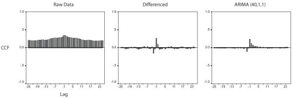
Cross correlation functions (CCF) calculated between sensors #70 and #54. The far left graph demonstrates values calculated between raw data, while the middle graph illustrates cross correlation calculated between differenced time series and the far right graph illustrates crosscorrelation calculated between time series after ARIMA (40,1,1) modeling. The positive CCF calculated using raw data reflects the autocorrelation structure of individual sensor time series. The middle CCF demonstrates the temporal focusing of cross correlation, though oscillatory waves achieve significance across the time lags. The CCF following ARIMA modeling illustrates a temporally focused interaction, though still exceeding the 95% confidence intervals as noted by the horizontal lines.

We found that the majority of pairwise PCC strengths across subjects and behavioral states were statistically significant well beyond Bonferroni correction for multiple comparisons (256 by 255 sensors by 30 000 time points or P < 1 × 10⁻¹¹). Using a threshold of absolute value of PCC strength greater than 0.1, all calculated P-values were less than 1 × 10⁻⁶⁶. At the same time, P-values were significantly inversely correlated with the absolute value of the PCC within subjects (range of r²: 0.11–0.2). Due to this high level of significance, we further verified the stability of identified interactions by comparing the results of analysis of the first half of each data set with results of the second half of each data set, retaining only those PCC values wherein each half was within 1% of the value calculated for the full data set. Given that PCC values of 0.1 account for a limited interaction despite statistical significance, we chose to use |PCC| ≥ 0.1 as an arbitrary threshold in displaying our results. Use of the |PCC| ≥ 0.1 threshold resulted in plotting from 369 to 913 pairwise interactions per subject of the 32 640 possible (mean ± SD; 620 ± 120), or approximately 1.9% of the interactions.

Fig. 5 illustrates positive and negative PCC-derived synchronous networks calculated from HD-EEG data in seven subjects during eyes-closed wakefulness as well as an averaged network map depicting the mean PCC value across all seven subjects. Here one sees positive clustering in a left fronto-temporal distribution (subjects 1, 3, 5, 7) and right parieto-occipital cluster (subjects 1, 2, 6 and, to a lesser extent, 4). Negative clustering is notably more variable across subjects. On average, the synchronization appears to be generally both localized and positive.

Figure 5.

Positive (black) and negative (red) synchronous networks synchronous networks of partial cross correlations during low artifact eyes-closed wakefulness (ECW).

Fig. 6 demonstrates diffuse and distant interactions, both positive and negative, taking place during REM sleep with minimal eye movements, showing greater variability among subjects. Positive right parieto-occipital clustering does appear to be present in three subjects (4, 6 and 7), with a negative correlate in two subjects (2 and 5). This increased intersubject variability is most evident in the considerable decrease in the number of significant partial correlations plotted in the seven subject average. Results from REM sleep with many eye movements (data not shown) were similar within subjects, save for considerably increased long-range and bilateral negative interactions with frontal channels.

Figure 6.

Positive (black) and negative (red) synchronous networks synchronous networks of partial cross correlations during low to no eye movement low artifact episodes of rapid-eye movement (REM) sleep.

With respect to SWS, Fig. 7 demonstrates localized clusters of left fronto-temporal positive PCCs in four subjects (1, 5, 6 and 7) and, to a lesser extent, in two others (3 and 4). Interestingly, due to significant artifacts present in early SWS stages for subject 4, those data depicted here represent a low-artifact data set from much later in the night (approximately 5 h 10 min) by comparison to the other subjects (1 h, range 30 min–1 h 50 min, with subject 2 at 1 h 50 min). While each subject of the seven also demonstrates more distant right parieto-temporo-occipital negative interactions, the degree of variability among subjects reduced significance below thresholds in the average map.

Figure 7.

Positive (black) and negative (red) synchronous networks synchronous networks of partial cross correlations during an early low artifact sample of Slow Wave Sleep (SWS1).

This SWS finding appears to be considerably attenuated in later SWS cycles, as shown for both individual maps and on average across subjects in Fig. 8. To further explore those changes in PCC strength over the course of a night of sleep, the significant interactions shown in the average first SWS sample were compared across separate and later SWS samples. All first sample SWS (SWS1) data were taken from cycle 1, except for in subject 4 for whom second cycle data were used as the first cycle was interrupted by multiple awakenings. These data were from 0.4 h to 3 h following sleep onset (mean 1.2 ± 0.8 h). For comparison, SWS2 data were taken from the latest and deepest low-artifact SWS cycle for each subject (from sleep onset: 5.2 ± 1.2 h; time from SWS1: 4.0 ± 1.5 h). Fig. 9 shows flying box plots of the mean values and distributions of z-transformed PCC strengths in (a) all subjects individually, and (b) across all subjects for the first and second SWS samples analysed. This shows that overall strength of PCCs in this region decreased from the earlier to later SWS cycles. As negative PCCs within this subset were sparse and inconsistent across subjects, both positive and negative data were included for all 237 interactions in each subject. In paired t-test, combined data and individual SWS2 means for each subject were significantly lower than SWS1 means, except for subject 4 (in whom the first sample set was collected 3 h into sleep).

Figure 8.

Positive (black) and negative (red) synchronous networks of partial cross correlations during a later low artifact sample of Slow Wave Sleep (SWS2).

Figure 9.

Flying box displays of the means and distributions of SWS1 and SWS2 z-transformed PCCs in A individual subjects and B combined across subjects, for those interactions significant on average across subjects in SWS1. Outliers and extreme outliers are not displayed. As negative PCCs within this subset were sparse and inconsistent across subjects, both positive and negative data were included for all 237 interactions in each subject.

In order to assess similarity across subjects in another manner, Fig. 10 is a composite figure of each behavioral state (formatted in rows) in which each column represents the number of subjects in whom each graphed interaction was present. The far left column shows interactions significant (|PCC| ≥ 0.1 and Bonferroni corrected) in at least two subjects, while the subsequent column shows interactions achieving the same in at least three of the seven subjects. The column furthest to the right depicts averages across all subjects, using the same thresholds.

Figure 10.

composite figure of behavior state (rows) and increasing commonality across subjects (columns).

There were more significant positive PCCs during waking than either SWS or REM (paired t-test, P < 0.001 and P < 0.01, respectively), and more significant negative PCCs during waking than REM (paired t-test, P < 0.03). In addition, the length of the average positive PCCs in waking (5.43 ± 0.35 cm) was significantly shorter than during SWS (7.20 ± 0.91 cm, paired t-test, P < 0.01) or REM (7.45 ± 1.33 cm, paired t-test, P < 0.02). The length of the average negative PCCs in waking (10.15 ± 1.23 cm) was significantly shorter than during REM (12.08 ± 1.97 cm, paired t-test, P < 0.05). A permutation-based cluster analysis showed a cluster of four electrodes over the right temporal cortex that had significantly higher mean PCC values (Nichols and Holmes, 2002).

In summary, the waking state demonstrates diffuse localized cortical interactions throughout much of the cortex across subjects. During REM sleep, localized interactions appear to lose strength (as reflected in PCC values) in favor of more distant interactions. Conversely, SWS reveals a localized cluster of left fronto-temporal connectivity, more consistent across subjects than clustering noted in either wakeful resting with eyes closed or during REM sleep.

DISCUSSION

We have used time series analysis methods originally developed for econometric study and recently applied to MEG data to identify synchronous dynamic networks in wakefulness and sleep using HD-EEG. Possible confounds of these findings and their interpretation include the potential correlative effects of spatial blurring and strong EMG signals upon the HD-EEG data. In addition, established encephalographic (ECG) techniques have focused upon the contribution of various frequency ranges, whereas the ARIMA modeling utilized in the present study precludes a clear delineation of which ECG frequencies contribute to the PCCs and which do not.

Regarding large current distributions and EMG signals, both would likely overwhelm simple cross-correlations between raw HD-EEG data. Similar concerns existed with respect to earlier work using MEG, and were mitigated first through the use of low-artifact data, ARIMA modeling and PCCs (Georgopoulos et al., 2007; Langheim et al., 2006). Widely distributed signals, such as SWS oscillations and muscle electrical activity, would introduce large and nearly equivalent correlations among multiple sensors. By selecting low-artifact data, EMG influences are grossly avoided. Furthermore, as described in the introduction, ARIMA modeling effectively removes the redundant information present in large sweeping signal changes. Finally, any surviving influences of large signal changes involving several sensors are further reduced by employing PCC analysis. PCC differs from simple cross-correlation in that only the strongest interaction among two time series (sensors) survives the analysis, while related interactions are subsequently removed from all other pairwise interactions involving either of those time series (sensors). Indeed, the comparison of frequent eye movement REM sleep to REM sleep with minimal eye movements demonstrated significant differences in long-range negative interactions among frontal channels, underscoring the need for selection of low-artifact data sets for analysis.

A drawback of the methodology used in the present study is the inability to clearly identify the contributions of various frequency bands to the synchronous networks. In fact, Butterworth filters are themselves ARIMA models, and the consequences of prewhitening data already prewhitened in portions of the frequency spectrum would result in model instability with unpredictable effects upon subsequent PCCs. One alternative, at least for lower frequency analysis, involves downsampling of the data to various Nyquist frequencies. For example, taking every 63^rd data point results in a sampling rate just under 8 Hz, for which no signal more rapid than 4 Hz may be detected. Decimating the data prior to ARIMA prewhitening avoids the aforementioned model instability that would arise from filtering prewhitened data, or prewhitening filtered data. While this approach could lose statistical power through reducing the number of time points used, Bonferonni correction of P-values could be employed to mitigate this confound. Indeed, by performing this analysis after downsampling the data to every 63^rd time point, the left fronto-temporal network identified in the results was no longer present, and identified functional connectivity was reduced to diffuse nearest-neighbor sensor pairs, which showed no substantial resemblance across subjects (data not shown). This suggests that ARIMA modeling removed the otherwise overwhelming correlations that would have come about through correlation of SWS oscillations in the delta range, while the interactions that contribute to the identified left fronto-temporal network take place at a frequency greater than 4 Hz.

The above concerns regarding strong signals and frequency band contributions not withstanding, the data revealed internal consistency of identified functional connectivity within subjects, and similarity across subjects during eyes-closed wakefulness. Furthermore, the positive clustering in a left fronto-temporal and right parieto-occipital distribution during quiet wakefulness is, overall, similar to previous results in MEG (Langheim et al., 2006), as well as fMRI (Hagmann et al., 2008) – gross methodological differences limiting the comparability of these techniques. Taken together, these results suggest that HD-EEG provides a valid approach to identifying functional connectivity in the form of highly synchronous dynamic networks. Of course, this is not enough to propose functional significance apart from this intrinsic validity, which would require specific behavioral manipulations such as localized learning.

On the other hand, these results show that this connectivity changes across behavioral states, i.e. wakefulness, REM sleep and SWS, as inferred via strength of synchronous positively- and negatively-correlated EEG potentials. While REM sleep showed increased variability across subjects and, in general, appeared somewhat consistent with the networks identified during eyes-closed wakefulness, SWS showed marked consistency across subjects in the form of a lateralized left fronto-temporal network of positively correlated synchronous EEG potentials. This lateralization has not been reported in prior functional connectivity analyses of EEG. In contrast, prior studies of EEG coherence indicated prominent intrahemispheric synchrony as compared with interhemispheric coherence in non-REM sleep (Achermann and Borbély, 1998). Those findings were largely independent of signal amplitude, with the most prominent coherence peak in the frequency range of sleep spindles. Later work by the same group identified an anterior increase in slow-wave activity in the first non-REM sleep period following a 40-h waking period for which the topographic display appeared biased to the left frontal region (Finelli et al., 2000), though that possible lateralization was not addressed. Explanations for why coherence measures have not identified the lateralization seen in the present study include the possibilities that the ARIMA method may be more sensitive than coherence measures, that the lateralized functional connectivity exists at frequencies greater than those typically analysed in coherence studies, or that the lateralized functional connectivity is not frequency specific.

While it is too early to state the significance of the lateralized findings in the current work, it may reflect a fundamental component of sleep. Though published data during sleep using PET do not suggest lateralized activity in these particular regions (Braun et al., 1997), as with fMRI, methodological differences challenge direct comparison across techniques. An intriguing hypothesis would suggest that these areas, associated with language use throughout the waking day, may be reactivated significantly more during sleep and detectable through the increased temporal resolution of HD-EEG. Interestingly, recent work showed that while slow waves during sleep may originate in either hemisphere, most appeared to originate in the left hemisphere (Murphy et al., 2009).

Although the present study does not address differences among populations, it does lay the groundwork for characterizing synchronous neural networks using prolonged and possibly ambulatory HD-EEG data acquisition followed by ARIMA modeling and PCC analysis. Should differences in functional connectivity during sleep be demonstrated across various psychopathologies, a new avenue of diagnostic testing and possible intervention may result.

REFERENCES

- Achermann P, Borbély AA. Coherence analysis of the human sleep electroencephalogram. Neuroscience. 1998;85:1195–1208. doi: 10.1016/s0306-4522(97)00692-1. [DOI] [PubMed] [Google Scholar]
- Box GEP, Jenkins GM. Time Series Analysis: Forecasting and Control. Holden Day; San Francisco, CA: 1970. [Google Scholar]
- Braun AR, Balkin TJ, Wesenten NJ, et al. Regional cerebral blood flow throughout the sleep-wake cycle. An H2(15)O PET study. Brain. 1997;120:1173–1197. doi: 10.1093/brain/120.7.1173. [DOI] [PubMed] [Google Scholar]
- Bullmore E, Sporns O. Complex brain networks: graph theoretical analysis of structural and functional systems. Nat. Rev. Neurosci. 2009;10:186–198. doi: 10.1038/nrn2575. [DOI] [PubMed] [Google Scholar]
- Damoiseaux JS, Greicius MD. Greater than the sum of its parts: a review of studies combining structural connectivity and resting-state functional connectivity. Brain Struct. Funct. 2009;213:525–533. doi: 10.1007/s00429-009-0208-6. [DOI] [PubMed] [Google Scholar]
- Finelli LA, Baumann H, Borbély AA, Achermann P. Dual electroencephalogram markers of human sleep homeostasis: correlation between theta activity in waking and slow-wave activity in sleep. Neuroscience. 2000;101:523–529. doi: 10.1016/s0306-4522(00)00409-7. [DOI] [PubMed] [Google Scholar]
- Georgopoulos AP, Karageorgiou E, Leuthold AC, et al. Synchronous neural interactions assessed by magnetoencephalography: a functional biomarker for brain disorders. J. Neural Engng. 2007;4:349–355. doi: 10.1088/1741-2560/4/4/001. [DOI] [PubMed] [Google Scholar]
- Georgopoulos AP, Tan HR, Lewis SM, et al. The synchronous neural interactions test as a functional neuromarker for post-traumatic stress disorder (PTSD): a robust classification method based on the bootstrap. J. Neural Engng. 2010;7:16 011. doi: 10.1088/1741-2560/7/1/016011. [DOI] [PubMed] [Google Scholar]
- Hagmann P, Cammoun L, Gigandet X, et al. Mapping the structural core of human cerebral cortex. PLoS Biol. 2008;6:e159. doi: 10.1371/journal.pbio.0060159. [DOI] [PMC free article] [PubMed] [Google Scholar]
- Langheim FJ, Leuthold AC, Georgopoulos AP. Synchronous dynamic brain networks revealed by magnetoencephalography. Proc. Natl Acad. Sci. USA. 2006;103:455–459. doi: 10.1073/pnas.0509623102. [DOI] [PMC free article] [PubMed] [Google Scholar]
- Leuthold AC, Langheim FJ, Lewis SM, Georgopoulos AP. Time series analysis of magnetoencephalographic data during copying. Exp. Brain Res. 2005;164:411–422. doi: 10.1007/s00221-005-2259-0. [DOI] [PubMed] [Google Scholar]
- Michel CM, Murray MM, Lantz G, Gonzalez S, Spinelli L, Grave De Peralta R. EEG source imaging. Clin. Neurophysiol. 2004;115:2195–2222. doi: 10.1016/j.clinph.2004.06.001. [DOI] [PubMed] [Google Scholar]
- Murphy M, Riedner BA, Huber R, Massimini M, Ferrarelli F, Tononi G. Source modeling sleep slow waves. Proc. Natl Acad. Sci. USA. 2009;106:1608–1613. doi: 10.1073/pnas.0807933106. [DOI] [PMC free article] [PubMed] [Google Scholar]
- Nichols TE, Holmes AP. Nonparametric permutation tests for functional neuroimaging: a primer with examples. Hum. Brain Mapp. 2002;15:1–25. doi: 10.1002/hbm.1058. [DOI] [PMC free article] [PubMed] [Google Scholar]
- Priestley MB. Spectral Analysis and Time Series. Academic Press; San Diego, CA: 1981. [Google Scholar]