Comparative analysis of Pareto surfaces in multi-criteria IMRT planning

Abstract

In the multi-criteria optimization approach to IMRT planning, a given dose distribution is evaluated by a number of convex objective functions that measure tumor coverage and sparing of the different organs at risk. Within this context optimizing the intensity profiles for any fixed set of beams yields a convex Pareto set in the objective space. However, if the number of beam directions and irradiation angles are included as free parameters in the formulation of the optimization problem, the resulting Pareto set becomes more intricate. In this work, a method is presented that allows for the comparison of two convex Pareto sets emerging from two distinct beam configuration choices. For the two competing beam settings, the non-dominated and the dominated points of the corresponding Pareto sets are identified and the distance between the two sets in the objective space is calculated and subsequently plotted. The obtained information enables the planner to decide if, for a given compromise, the current beam setup is optimal. He may then re-adjust his choice accordingly during navigation. The method is applied to an artificial case and two clinical head neck cases. In all cases no configuration is dominating its competitor over the whole Pareto set. For example, in one of the head neck cases a seven-beam configuration turns out to be superior to a nine-beam configuration if the highest priority is the sparing of the spinal cord. The presented method of comparing Pareto sets is not restricted to comparing different beam angle configurations, but will allow for more comprehensive comparisons of competing treatment techniques (e.g. photons versus protons) than with the classical method of comparing single treatment plans.

1. Introduction

1.1. Background

In intensity modulated photon radiation therapy, the quality of a treatment plan mainly depends on two types of parameters: the setup of the beam directions determined by the number and angles, and the values of the beamlet intensities for each of the chosen directions. Once the beam directions are fixed, the beamlet intensity optimization can be carried out in a multi-criteria fashion if the criterion functions and constraints are chosen to be convex (Küfer et al 2000,Cotrutz et al 2001, Lahanas et al 2003, Thieke et al 2007). This is done by approximating the Pareto surface, e.g. by a sandwiching scheme (Solanki et al 1993, Klamroth et al 2002, Craft et al 2006, Serna et al 2009). Within this procedure, the search for each Pareto optimal solution is a convex problem and thus can be solved to the global optimum by gradient-based methods. Subsequently the user can navigate on the obtained approximation of the Pareto surface, guided by the properties of the corresponding dose distributions and dose volume histograms (Monz et al 2008).

The inclusion of the beam direction parameters in the optimization process is difficult, however, as the resulting problems are highly non-convex and therefore the application of deterministic gradient-based solvers becomes infeasible. As a consequence the set of possible beam directions is usually discretized, turning the IMRT planning problem into a mixed integer problem (Lee et al 2003). Combinatorial methods such as branch and bound may then be applied to find a good set of beam directions.

The loss of convexity also carries over to the properties of the Pareto surface, making it a challenging task to find a suitable approximation scheme. However, we can preserve convexity at least locally (see figure 1). To this aim we exploit the aforementioned fact that once we fix the discrete parameters that determine the beam configuration, the problem of optimizing the beamlet intensities is convex and continuous. Each convex Pareto surface that is the result of such a lower level problem is called a `patch'. The Pareto surface of the larger problem then consists of the non-dominated parts of all the patches.

Figure 1.

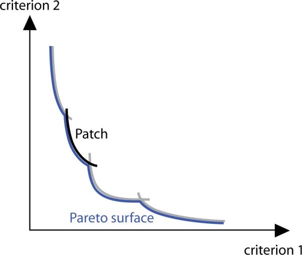
For each beam configuration, there is a convex Pareto set (a `patch') whose points are the images of the Pareto optimal beamlet intensity profiles. The Pareto surface of the multi-criteria IMRT planning problem is the locally convex union of the non-dominated parts of these patches.

Resolving the difficulties caused by the non-convexity and eventually extending the multi-criteria planning paradigm for IMRT to include the choice of beam directions is the goal of ongoing research. Only a successful integration of the beam directions in the planning framework allows for a complete exploration of all possible plans, and only a multi-criteria approach accompanied by an intuitive navigation support guarantees that the optimization appropriately reflects the assessment and knowledge of the planner.

1.2. Purpose

In this paper, we present a method to identify and visualize the non-dominated part of a given patch. The obtained knowledge may be used to assess whether the investigated patch significantly contributes to the Pareto surface. More importantly, it is suited to guide the user in choosing the appropriate beam configuration during navigation.

For the purpose of easy demonstration, we limit ourselves to the consideration of two patches corresponding to two different beam configurations here, although the presented technique can be applied to any finite number of patches. After giving a short introduction to the principles of multi-criteria optimization, we briefly touch the subject of the Pareto surface approximation. We then develop a computational method to assess the distance between two patches at a point, which allows us to identify the parts where one patch dominates the other and vice versa.

In section 3, the method is applied to one artificial and two clinical cases. We illustrate how the presented technique provides the user with the information needed to choose among the two alternatives during navigation.

2. Material and methods

2.1. Pareto optimality and Pareto surface approximation

The multi-criteria optimization approach tries to tackle problems where the quality of every potential solution depends on more than one attribute. For each choice of parameters, the different criteria are measured by a set of N objective functions. The attained values constitute the so-called criterion vector. However, in general there is no parameter configuration such that the corresponding criterion vector is optimal in every component. Thus, instead of looking for an unequivocally best solution one tries to find a set of optimal compromises.

The mathematical term that describes such an optimal compromise is the Pareto optimality. A parameter vector x is said to be Pareto optimal if there is no other vector y with f_k(y) ≤ f_k(x) for all k and at least one index i with f_i(y) < f_i(x). The criterion vector f(x) of a Pareto optimal point x is called a non-dominated point. The set of all non-dominated points is called the Pareto set or the Pareto surface.

In IMRT, the convex problem of computing the beamlet intensities for a fixed configuration of irradiation angles has been successfully tackled with a multi-criteria approach (Küfer et al 2000). For a specific beam configuration, let $\mathbf{x}\in {\mathbb{R}}_{+}^n$ denote the corresponding vector of beamlet intensities. Each choice of x leads to a certain dose distribution d(x) that in turn determines the values of the criterion functions f(x). To limit the approximation scheme to clinically relevant plans, the criterion functions are usually bounded from above. Also, additional constraints that are not related to the criterion functions may be given by convex functions g(x). The problem then reads as

$$\mathrm{v}-\min \{\mathbf{f}\left(\mathbf{x}\right)\mid \mathbf{f}\left(\mathbf{x}\right)\le \mathbf{b},\mathbf{g}\left(\mathbf{x}\right)\le \mathbf{b}\prime ,\mathbf{x}\ge 0\}.$$ (1)

Typical criterion functions for IMRT include TCP and NTCP models, generalized EUD (Niemierko 1999) and tail EUDs (Bortfeld et al 2008) as well as one- or two-sided deviations from the prescribed dose. We will use Niemierko's EUD concept, with the pEUD defined as

$$\mathrm{pEDU}\left(\mathbf{d}\left(\mathbf{x}\right)\right)={\left(\frac{1}{\mid V\mid }\sum _{i\in V}{d}_i{\left(\mathbf{x}\right)}^p\right)}^{\frac{1}{p}},$$ (2)

where V denotes the set of voxels of the corresponding structure (typically an organ at risk), d_i is the dose delivered to voxel i, and p is a parameter in [1, ∞).

For the approximation of the Pareto surface, the sandwiching scheme described by Serna et al (2009) is used. Given a set of k plans, the convex combination of the corresponding criterion vectors provides a pessimistic approximation of the Pareto surface, while the polytope confined by the set of tangent planes at these points delivers an upper bound for the quality of plans that can be reached. Both bounds are updated by the addition of plans at points where the distance between outer and inner approximations is largest until the desired approximation quality is reached (see figure 2). The result is a set of criterion vectors which approximate the Pareto surface with the desired quality.

Figure 2.

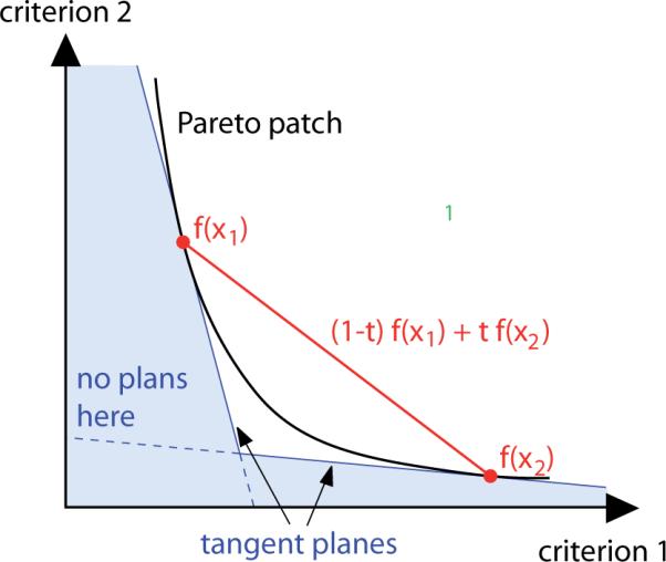
To approximate the Pareto frontier a sandwiching scheme is used. The two red dots denote the criterion vectors of two computed plans. A lower bound for the Pareto surface with respect to plan quality is given by the convex combinations of the two plans' criterion vectors: (1 − t)f(x₁) + tf(x₂) (red line). The blue area is guaranteed to contain no feasible criterion vectors as the two plans' tangent planes to the Pareto surface provide an upper bound for the Pareto set with respect to plan quality.

2.2. Comparison of two patches by calculating the distance function

Imagine a planner who has two possible options for the beam setup, the configurations Φ and Ψ. He provisionally settles on Φ and finishes the navigation process on the corresponding patch $P_{\Phi }\subseteq {\mathbb{R}}^N$. He may now wonder if he can improve the found criterion vector by switching to the configuration Ψ. He may only accept another solution if it is as least as good as the old one in every criterion, however. In the following, we develop the appropriate mathematical scheme to pursuit this strategy. (In clinical practice there might be cases where the planner may only want to improve on a subset of the criteria, while others are allowed to worsen. In this case the patches have to be projected onto the subspace corresponding to the criteria that should be improved, and the method applied on the projections. The planner can ensure that the other criteria are not worsened too much by removing unacceptable solutions from the patches before the projection is carried out.)

Let us assume that P_Ψ is approximated by points r₁, r₂,…, r_m. The question if such a dominating point on P_Ψ exists can be answered by solving an appropriate linear program. More precisely, for a given criterion vector p on P_Φ and a given direction $\mathbf{n}\in {\mathbb{R}}_{+}^N$ with ||n|| = 1 one can calculate the distance between the two patches along the line that passes through p the n-direction (see figure 3) by solving the linear program

$$\begin{array}{cc}\hfill & \min \alpha \mathrm{s}.\mathrm{t}.\hfill \\ \hfill \mathbf{p}+\alpha \mathbf{n}& \ge \sum _{i=1}^m{\lambda }_i{\mathbf{r}}_i\hfill \\ \hfill \sum _{i=1}^m{\lambda }_i& \ge 1\hfill \\ \hfill {\lambda }_i& \ge 0(i=1,\dots ,m).\hfill \end{array}$$ (3)

Figure 3.

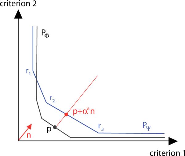
The distance between the two approximated patches P_Φ and P_Ψ in the criterion vector p is determined by computing the minimal α such that p + αn is a point of the set confined by the approximation of P_Ψ.

Let the obtained minimum be α*. For α* > 0, p is not dominated by any point of P_Ψ, which means that the found solution cannot be improved in one criterion without worsening another one. On the other hand, for α* < 0 the point p + α*n ε P_Ψ dominates p. Then the plan can be improved by changing the beam setup to the configuration Ψ.

The choice of n is irrelevant for deciding whether p is dominated or not. However, it determines the measured distance α*. Within the examples of section 3 we chose n to be the normalized all-one vector. In our examination of the artificial horse shoe target case this is natural as it reflects the weighting of the objectives. In the clinical head neck examples the comparison is invoked after the user has already navigated to a solution that reflects his preferences. Hence we can assume that, at this point, the aim is general improvement of the found solution with no particular emphasis on any of the criteria. Nevertheless, other choices of n are feasible and may be better suited situationally.

The knowledge about the dominating patch in p is not sufficient, however, as long as the navigation process is not completed. If the planner fixes a beam configuration at some point but subsequently continues to navigate on the chosen patch, he may unknowingly end up at a point where this patch is not dominating any longer. We therefore want to extend the comparison to include the area around p. This would enable the user to tell beforehand whether a direction is `safe to navigate' or if a change of the beam configuration is needed to stay on the Pareto set.

To extend the comparison to the area around p we define a grid on the hyper plane which runs through p and is orthogonal to n (see figure 4). Having established the grid around p, we then compute the distance between the patches P_Φ and P_Ψ along the lines that run in the n-direction through each of the points of the grid. To this end we solve one linear program for each grid point and patch; calculating the difference between the two results, we obtain the distance d between the two patches at the grid point. Whenever d < 0, P_Φ dominates at the considered grid point while if d > 0, the patch P_Ψ dominates. The geometrical properties of the patches guarantee that the projection of the Pareto optimal points on the hyper plane is bijective and also that exactly one of the patches dominates at each grid point provided that d ≠ 0 holds (see the appendix for more details).

Figure 4.

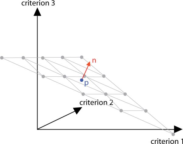
Around p, we define a grid in the plane orthogonal to n. In the three-dimensional case, the grid is triangularly shaped and consists of equidistantly spaced convex combinations of the corner points.

3. Results

In the following, we will analyze one artificial and two clinical cases with the help of the comparison scheme presented in the previous section. In the discussion of the clinical cases multiple criteria were merged to allow a visual representation of the distance function. The difference between the two patches at the grid points is plotted as a map or as a two-dimensional surface. In the map plot the non-dominated parts are color-coded: red means the first patch is dominating, blue means the second patch is dominating, and green denotes the indifference. The edges of the triangle in the map plot correspond to the three conflicting criteria in the sense that moving toward one edge means improving the corresponding criteria at the expense of the other two (see figure 5).

Figure 5.

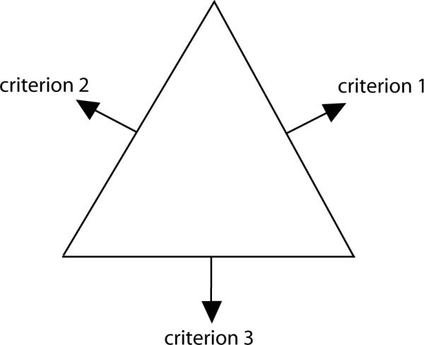
The alignment of the three criteria in the map plot. Moving toward the edge of criterion i equates to lowering the corresponding objective f_i at the expense of the other objectives.

3.1. Artificial horse shoe target

The horse shoe target case is a two-dimensional abstraction of a concave tumor growing around an organ at risk. For our testing purposes, the conflicting planning goals were modeled by a standard deviation on the target (first criterion), a pEUD with exponent 5 for the organ at risk (second criterion) and a pEUD with exponent 2 for the surrounding tissue (third criterion). The target dose prescription was set to 60 Gy.

We chose two differing beam configurations that seemed attractive: an equidistant five beam configuration that presumably allows for a smooth coverage of the tumor, and a configuration that was found with a heuristic approach (Azizi Sultan (2006), see figure 6).

Figure 6.

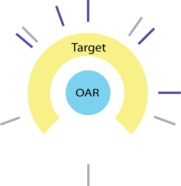
The two competing beam configurations for the horse shoe target case: heuristically obtained (violet) and equiangular (gray).

For each beam configuration, Pareto optimal solutions were computed to approximate the corresponding patch within an error bound of 1%. The grid was centered at the optimal solution of the equibalanced weighted sum problem

$$\min \{f_1\left(\mathbf{x}\right)+f_2\left(\mathbf{x}\right)+f_3\left(\mathbf{x}\right)\mid \mathbf{x}\ge 0\}$$ (4)

for the heuristically obtained beam setting. The grid parameters C and M were chosen to be 50 and 32, respectively. For the solution of the linear programs, the simplex algorithm of MATLAB was used.

The results are depicted in figures 7 and 8. Around the center of the plot, the criterion vectors of the first, heuristically obtained beam configuration are non-dominated. The difference in the scalarized objective function value at this point is −7.0. However, this configuration is not superior for any weighting of the different criteria. On one hand we can further improve the objective associated with the organ at risk at the expense of the tissue objective without navigating out of the non-dominated area. On the other hand, further improving the tissue objective leads to areas where the two beam configurations are equal, or where the equidistant setting is the better choice.

Figure 7.

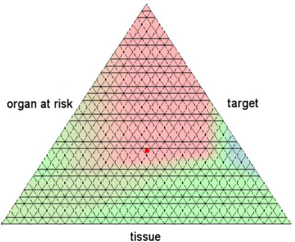
The map plot of the distance function for the horse shoe target case. Areas where the heuristically obtained beam configuration is dominating are colored in red, and those where the equidistant setting dominates are colored in blue. The red dot denotes the solution for the heuristic beam setting for an equal weighting of all three criteria.

Figure 8.

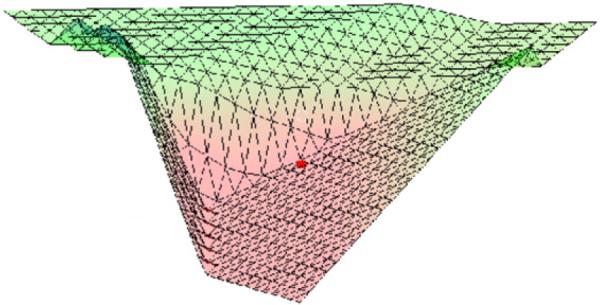
Surface plot of the distance function for the horse shoe target case. For a better visualization, the upper corner of the triangle in figure 7 is in front.

If one wants to make sure that the planner stays within the non-dominated area of his chosen beam setting but does not want to bias him toward a certain trade-off, one can compute a maximal radius such that navigation is safe within the encompassed area. A natural definition for the radius is

$$r_{\max }=\max \left\{r\in \mathbb{R}\mid \mathrm{q}\mathrm{non}-\mathrm{dominated}\mathrm{whenever}\sum _{k=1}^n\mid p_k-q_k\mid \le r\right\}.$$ (5)

In the current example, the computed radius r_max was 22.3. Within this area, the average benefit of the heuristically obtained beam setting was −4.5.

3.2. Clinical head neck case I

In the first clinical head neck case investigated here, the tumor is in the process of retreat and the spinal cord has already received high doses in previous treatments. Thus sparing the spinal cord has the highest priority. It should nowhere receive more than 5 Gy, and its mean dose should not be higher than 2.5 Gy. The model comprises objectives to punish under dosage in the targets, mean dose objectives for mandible and parotids and two pEUD objectives affiliated with the spinal cord.

Again, the question that the Pareto front comparison routine should help to answer is which beam setting should be used. The configurations in question are an equiangular seven-or nine-beam configuration (see figure 9). However, to obtain a three-dimensional plot different objectives have to be merged. Thus we combine the under dose objectives of the two targets into a first criterion, the mean doses of the parotids and the mandible into a second criterion and the two EUDs associated with the spinal cord into a third criterion.

Figure 9.

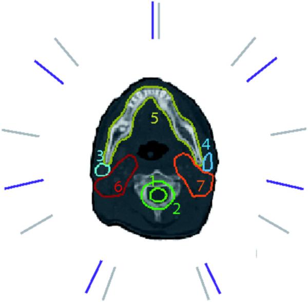
Seven-beam (violet) and nine-beam (gray) configuration for the head neck case I. (1) spinal cord, (2) cord plus, (3) right parotid, (4) left parotid, (5) mandible, (6) first target, and (7) second target.

The strict demand with regard to the sparing of the spinal cord limits the region of the Pareto frontier the physician will be interested in. In figure 10, the distance function is plotted for the interesting section. The physician discovers that his current solution (point 1), which was calculated with the seven-beam setting, is dominated and he should—with his current preferences—switch to the nine-beam configuration.

Figure 10.

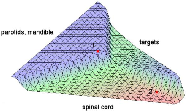
Surface plot of the distance function of the head neck case I. The solution with the seven-beam setting plotted in red is dominated by the nine-beam setting at point 1, but dominates at point 2.

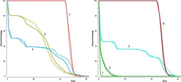
Interestingly, the seven-beam configuration is not worse than the nine-beam configuration in the southeast region of the plot, however. If the physician decides to further improve the spinal cord DVHs, he will navigate into a region where the nine-beam configuration is no longer dominating. For example, this phenomenon applies at the marked point 2. In figure 11, the DVH curves at this point are depicted for both beam configurations. They show that the seven-beam setting is indeed superior.

Figure 11.

DVH curves for the seven-beam setting and nine-beam setting (dotted) at point 2 in figure 10. (1) spinal cord, (2) cord plus, (3) right parotid, (4) left parotid, (5) mandible, (6) first target, and (7) second target.

However, the physician may not want to combine the objectives for the mandible and the two parotids into a single criterion, as he may be interested in all organs individually. He can still use the algorithm to compare the Pareto sets in five-dimensional space, although the distance function cannot be plotted. The comparison is made around the seven-beam solution in figure 11 of which we already know that it dominates in the three-dimensional projection discussed above. It turns out that this solution also dominates if the five-dimensional Pareto sets of the seven- and nine-beam configuration are compared. The numerical results are depicted in tables 1 and 2.

Table 1.

Numerical results of the comparison in 5D for the head neck case I around the seven-beam solution in figure 11 with parameters C = 50 and M = 32. Each face of the grid simplex is affiliated with one criterion: the criterion improves with decreasing distance to the face (see figure 5 and explanation). The negative value for the objective function difference indicates that the chosen seven-beam configuration stays superior if the spinal cord objective is further improved. If target coverage should be significantly improved however, a switch to the nine-beam configuration is indicated.

		Center of faces
	Grid center	Target	Mandible	Left parotid	Right parotid	Spinal cord
Δ objective	−7.9	10.0	0.03	3.5	−1.7	−13.2
Dominates?	+	−	0	−	+	+

Table 2.

Numerical results of the comparison in 5D for the head neck case I. The radius of the non-dominated area is calculated by formula (5).

Quantity	Value
Δ objective in grid center	−7.9
Radius of non-dominated area	4.4
Average Δ objective in non-dominated area	−4.2

3.3. Clinical head neck case II

In the second clinical head neck case, the physician is particularly interested in sparing one of the parotids, as this makes a significant benefit in the quality of life for the patient. This goal is reflected in our modeling by a strict over dose objective imposed on the left parotid. Again, we will compare two beam configurations: the first setup was selected by the physician to fit the specific treatment goals as well as the shape of the tumor, and the second one is an equiangular nine-beam setting (see figure 12).

Figure 12.

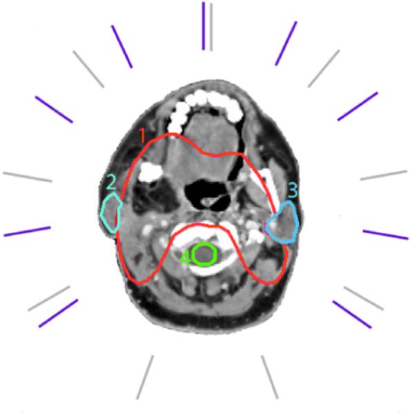
Case specific (violet) and equiangular (gray) beam directions for the head neck case II. (1) target, (2) right parotid, (3) left parotid, and (4) spinal cord.

Again we have to merge the objectives to gain a visualized representation of the difference function. The objectives affiliated with tumor coverage were combined to a first criterion, all objectives corresponding to organs at risk except the left parotid were merged in a second criterion, and the over dose objective for the left parotid yields a third criterion.

The DVHs of a good solution achieved with the case specific beam configuration are depicted in figure 13. We want to find out if the chosen beam setting is indeed better than the equidistant one in the vicinity of this solution. Figure 14 shows that this is the case: around the solution point the patch corresponding to the case specific setup dominates. The difference in the scalarized objective function value at the point is −7.6; the maximal radius as defined in equation (5) is 17.2.

Figure 13.

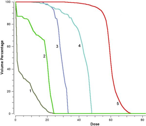
The DVH curves for the head neck case II, obtained with a case specific beam setting. (1) brain stem, (2) spinal cord, (3) left parotid, (4) right parotid, and (5) target.

Figure 14.

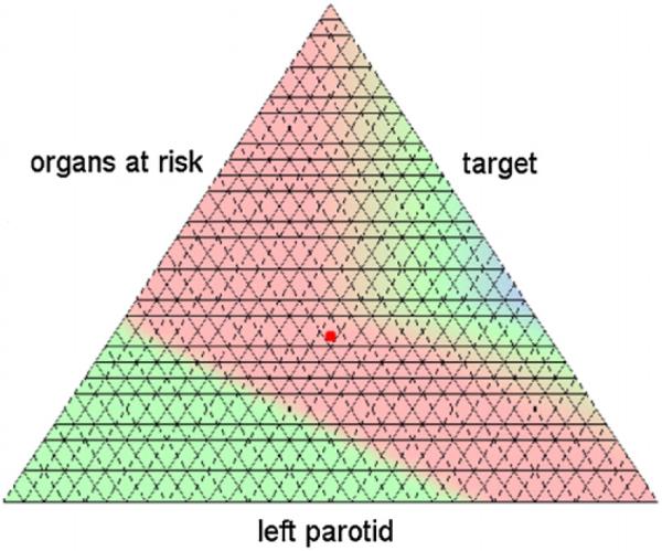
Map plot of the distance function for the head neck case II for parameters C = 50 and M = 32. The case specific beam setup is dominating in and around the solution depicted figure 13 (red point).

4. Discussion

We introduced a numerical method to compare convex Pareto surfaces and applied it to support beam setup choice in IMRT planning. For the method to work, it is required that the convex patches are situated in the same criterion space. It was shown by Ottosson et al (2009) and Benedek (2009) that Pareto surfaces can successfully be applied to compare different radiation modalities (e.g. photons versus protons) or different treatment planning systems or delivery techniques. For all these cases, the application of the presented method is feasible as long as the objective functions remain unaltered over the set of the evaluated modalities. This will allow for more comprehensive comparisons of competing treatment techniques than the classical approach of comparing a single plan from each modality.

The method requires the Pareto surface to be approximated by some approximation scheme as described in section 2.1. As a rule of thumb, only a comparatively small number of points (N +1 in an N-dimensional criterion space) are needed to achieve a good approximation quality. Hence the computation time is only marginally impaired by this step if N gets larger. However, the number of grid points needed for the resolution of the grid to stay the same grows exponentially for increasing N. Because of this exponential increase at the grid points needed and thus in the number of optimization problems that have to be solved, the method is not well suited for high dimensions (>10).

However, in our experience even complex cases with many objectives often have a limited number of really `strong' competing objectives between which the planner has to decide according to clinical importance, while other objectives are well within their tolerance for all plan alternatives. In this case, the comparison can be confined to the competing criteria. Therefore we think that the method as proposed is useful both for critical planning problems with a limited number of objectives (e.g. irradiation of paraspinal tumors) and for planning problems with more objectives.

Part of our future work will be on ways of visualizing the results for dimensions higher than 3 without the need of merging objectives. We will also investigate whether the described method can be used to automatically determine the optimal patch during navigation on a patched Pareto surface. This could be made completely transparent to the user, so that the treatment planner will no longer have to actively choose from different setups and still will always see the best available option for the patient.

5. Conclusion

We presented a novel method that allows the comparison of two convex Pareto sets by evaluating their distance in the criterion space. We showed in three exemplary cases that the visualized distance function can be a helpful tool during navigation on the Pareto set. The comparison can lead to new insights and thus to a more informed assessment of the beam setup choices.

Appendix

In the following, the construction of the grid introduced in section 2.2 and the calculation of the distance at the grid points are depicted in more detail.

Let us assume that we have a multi-criteria IMRT problem with N objectives and two competing beam settings. The corresponding patches P_Φ and P_Ψ are approximated by the points p₁, p₂, …, p_l and r₁, r₂, …, r_m, respectively. Our aim is to compare the two patches P_Φ and P_Ψ in the neighborhood of some point p on P_Φ. We choose a direction n = (n₁, …, n_N) ∈ $\mathbf{n}=(n_1,\dots ,n_N)\in {\mathbb{R}}_{+}^N$ with ∥n∥ = 1 and now want to define a grid on the plane that runs orthogonal to n through p. The grid should be centered at p and expand over the surrounding region that the user is interested in.

Let e_k denote the kth unit vector of the criterion space and set

$${\tilde{\mathbf{e}}}_k=\frac{1}{n_k}{\mathbf{e}}_k.$$ (A.1)

The barycenter of the vectors ẽ_k is

$$\mathbf{u}=\frac{1}{N}\sum _{k=1}^N{\tilde{\mathbf{e}}}_k.$$ (A.2)

Then for some positive real C and integer M the grid is defined by

$${\Lambda }_{C,M}=\left\{\mathbf{q}\in {\mathbb{R}}^N\mid \mathbf{q}=\mathbf{p}+C\left(\sum _{k=1}^N\frac{{\eta }_k}{M}{\tilde{\mathbf{e}}}_k-\mathbf{u}\right),{\eta }_k\in {\mathbb{N}}_0,\sum _{k=1}^n{\eta }_k=M\right\},$$ (A.3)

that is, by a shifted and scaled discrete set of convex combinations of the vectors ẽ_k (see figure A1). The parameter C controls the spread of the grid and thus the size of the region that is compared, while M determines the number of grid points (there are M + 1 grid points along an edge of the grid).

Having established the grid, we now compute the distance between the patches P_Φ and P_Ψ along the lines that run in the n-direction through each of the points of Λ_C,M. To this end we solve the linear programs

$$\begin{array}{cc}\hfill & \min \alpha \mathrm{s}.\mathrm{t}.\hfill \\ \hfill \mathbf{q}+\alpha \mathbf{n}& \ge \sum _{i=1}^l{\lambda }_i{\mathbf{p}}_i\hfill \\ \hfill \sum _{i=1}^l{\lambda }_i& \ge 1\hfill \\ \hfill {\lambda }_i& \ge 0(i=1,\dots ,l)\hfill \end{array}$$ (A.4)

and

$$\begin{array}{cc}\hfill & \min \beta \mathrm{s}.\mathrm{t}.\hfill \\ \hfill \mathbf{q}+\beta \mathbf{n}& \ge \sum _{i=1}^m{\lambda }_i{\mathbf{r}}_i\hfill \\ \hfill \sum _{i=1}^m{\lambda }_i& \ge 1\hfill \\ \hfill {\lambda }_i& \ge 0(i=1,\dots ,m)\hfill \end{array}$$ (A.5)

and calculate the difference d = α − β for each grid point q. Whenever d < 0, the point q + α * n ∈ P_Φ is non-dominated itself and dominates q + β * n ∈ P_Ψ, while if d > 0, the reverse situation holds.

Figure A1.

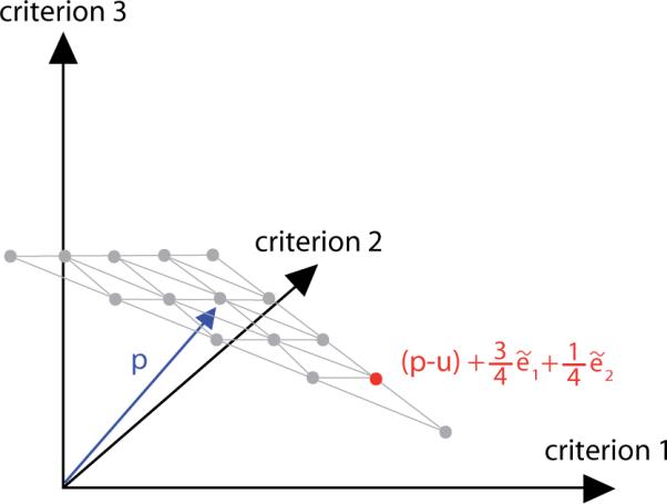
Let C = 1. We define a grid in the plane that runs parallel to the one spanned by the weighted unit vectors ${\tilde{\mathbf{e}}}_k$, with the barycenter of the former shifted to p. The grid consists of equally spaced convex combinations of the corner points $\left\{(\mathbf{p}-\mathbf{u})+{\tilde{\mathbf{e}}}_k\mid k=1,\dots ,N\right\}$.

References

- Azizi Sultan A S. PhD Thesis. Department of Mathematics, Technical University of Kaiserslautern; Germany: 2006. Optimization of beam orientations in intensity modulated radiation therapy planning. [Google Scholar]
- Benedek H. Master of Science Thesis. University of Lund; Sweden: 2009. Comparison of IMRT delivery techniques and helical Tomo therapy using Pareto front evaluation. [Google Scholar]
- Bortfeld TR, Craft D, Dempsey JF, Halabi T, Romeijn HE. Evaluating target cold spots by the use of tail EUDs. Int. J. Radiat. Oncol. Biol. Phys. 2008;71:880–9. doi: 10.1016/j.ijrobp.2008.01.049. [DOI] [PMC free article] [PubMed] [Google Scholar]
- Cotrutz C, Lahanas M, Kappas C, Baltas D. A multiobjective gradient-based dose optimization algorithm for external beam conformal radiotherapy. Phys. Med. Biol. 2001;46:2161–75. doi: 10.1088/0031-9155/46/8/309. [DOI] [PubMed] [Google Scholar]
- Craft D, Halabi TF, Shih HA, Bortfeld TR. Approximating convex Pareto surfaces in multiobjective radiotherapy planning. Med. Phys. 2006;33:3399–407. doi: 10.1118/1.2335486. [DOI] [PubMed] [Google Scholar]
- Klamroth K, Tind J, Wiecek MM. Unbiased approximation in multicriteria optimization. Math. Methods Oper. Res. 2002;56:413–37. [Google Scholar]
- Küfer KH, Hamacher HW, Bortfeld TR. A multicriteria optimization approach for inverse radiotherapy planning. Proc. 13th ICCR; Heidelberg. 2000. pp. 26–9. 2000. [Google Scholar]
- Lahanas M, Schreibmann E, Baltas D. Multiobjective inverse planning for intensity modulated radiotherapy with constraint-free gradient-based optimization algorithms. Phys. Med. Biol. 2003;48:2843–71. doi: 10.1088/0031-9155/48/17/308. [DOI] [PubMed] [Google Scholar]
- Lee E, Fox T, Crocker I. Integer programming applied to intensity-modulated radiation therapy treatment planning. Ann. Oper. Res. 2003;119:165–81. [Google Scholar]
- Monz M, Küfer KH, Bortfeld TR, Thieke C. Pareto navigation—algorithmic foundation of interactive multi-criteria IMRT planning. Phys. Med. Biol. 2008;53:985–98. doi: 10.1088/0031-9155/53/4/011. [DOI] [PubMed] [Google Scholar]
- Niemierko A. A generalized concept of equivalent uniform dose. Med. Phys. 1999;26:1100. doi: 10.1118/1.598063. [DOI] [PubMed] [Google Scholar]
- Ottosson RO, Engström PE, Sjöström D, Behrens CF, Karlsson A, Knöös T, Ceberg C. The feasibility of using Pareto fronts for comparison of treatment planning systems and delivery techniques. Acta Oncol. 2009;48:233–7. doi: 10.1080/02841860802251559. [DOI] [PubMed] [Google Scholar]
- Serna JI, Monz M, Küfer KH, Thieke C. Trade off bounds for the Pareto surface approximation in multi-criteria IMRT planning. Phys. Med. Biol. 2009;54:6299–311. doi: 10.1088/0031-9155/54/20/018. [DOI] [PubMed] [Google Scholar]
- Solanki RS, Appino PA, Cohon JL. Approximating the noninferior set in multiobjective linear programming problems. Eur. J. Oper. Res. 1993;68:356–73. [Google Scholar]
- Thieke C, Küfer KH, Monz M, Scherrer A, Alonso FV, Oelfke U, Huber P, Debus J, Bortfeld TR. A new concept for interactive radiotherapy planning with multicriteria optimization: first clinical evaluation. Radiother. Oncol. 2007;85:292–8. doi: 10.1016/j.radonc.2007.06.020. [DOI] [PubMed] [Google Scholar]