An Introduction to Tree-Structured Modeling with Application to Quality of Life (QOL) Data

Abstract

Background

Investigators addressing nursing research are faced increasingly with the need to analyze data that involve variables of mixed types and are characterized by complex nonlinearity and interactions. Tree-based methods, also called recursive partitioning, are gaining popularity in various fields. In addition to efficiency and flexibility in handling multifaceted data, tree-based methods offer ease of interpretation.

Objectives

To introduce tree-based methods, discuss their advantages and pitfalls in application, and describe their potential use in nursing research.

Method

In this paper, (a) an introduction to tree-structured methods is presented, (b) the technique is illustrated via quality of life (QOL) data collected in the Breast Cancer Education Intervention (BCEI) study, and (c) implications for their potential use in nursing research are discussed.

Discussion

As illustrated by the QOL analysis example, tree methods generate interesting and easily understood findings that cannot be uncovered via traditional linear regression analysis. The expanding breadth and complexity of nursing research may entail the use of new tools to improve efficiency and gain new insights. In certain situations, tree-based methods offer an attractive approach that help address such needs.

Investigators addressing nursing research frequently undertake composite research questions. The involved statistical analysis has become more and more demanding as the collected data are often characterized by variables of mixed types and complex nonlinearity and interactions that challenge the assumptions of common analytic methods.

Tree-based methods, also called recursive partitioning, are effective in handling multifaceted data, and are gaining acceptance as a methodology for addressing data complexity, which renders them particularly popular in biomedical applications. See Crichton, Hinde, and Marchini (1997); Fan, Su, Levine, Nunn, and LeBlanc (2006); Hess, Abbruzzese, Lenzi, Raber, and Abbruzzese (1999); Mair, Smidt, Lechleitner, Dienstl, and Puschendorf (1995); McKenzie et al. (1993); Steffann, Feyereisen, Kerbrat, Romana, and Frydman (2005); and Vlahou, Schorge, Gregory, and Coleman (2003) for some examples in medical prognosis and diagnosis. The hierarchical tree structures are useful for creating model-based clinical decision rules that mimic the way of assigning prognosis or diagnosis by clinicians.

Tree modeling has gained so much popularity that its implementation has been made available in all major statistical computing packages. In R (R Development Core Team, 2010), two main packages are available, tree and rpart; in SAS, tree analysis can be conducted using PROC Split; it is also implemented in SPSS, in the Decision Trees module. Now it is possible to perform tree analysis without a deep understanding of detailed steps in this algorithmic procedure.

With great flexibility and easy interpretation, tree-structured modeling can be applicable to nursing research. With the advent of computing facilities and database technology, huge amounts of high-dimensional data with multifaceted structures are being collected in the nursing field. An increasing amount of nursing research and publications are based on primary or secondary analysis of large national surveys or web-based databases (e.g., Cho, Ketefian, Barkauskas, & Smith, 2003; Duffy, 2006; Henry, 1995; Lange & Jacox, 2004). Tree-structured methods are among the fundamental tools for mining or exploring large observational data.

The purpose of this paper is to provide an informative and accessible introduction to tree modeling, discuss the advantages and pitfalls of this emerging and cutting-edge technique, and demonstrate a tree application in analyzing quality of life (QOL) data in a Breast Cancer Education Intervention (BCEI) trial.

History of Tree Methods

The history of tree methods can be traced back to Morgan and Sonquist (1963), who initiated the idea and implemented the first tree software – the Automatic Interaction Detection (AID). Tree models have been made popular and widely applicable by the introduction of the Classification and Regression Trees (CART; Breiman, Friedman, Olshen, & Stone, 1984) methodology. The tree size selection problem and many other practical issues in tree applications are addressed successfully with CART. The CART paradigm remains the current standard of tree modeling. Other noteworthy tree implementations include CHi-squared Automatic Interaction Detector (CHAID) by Kass (1980) and C4.5 by Quinlan (1993). There are typically two types of trees: regression trees when the outcome or response variable is continuous and classification trees (also known as decision trees) when the outcome is binary or categorical. From a statistical perspective, regression itself is a broader concept that includes the classification problem as a special case. In fact, regression trees have been extended to handle many other types of responses, such as count data (Choi, Ahn, & Chen, 2005; Lee & Jin, 2006), censored survival times (LeBlanc & Crowley, 1993), longitudinal data (Lee, 2005; Segal, 1992), and times series (Adak, 1998). The focus of this paper is on regression trees where the outcome is the continuous variable and the CART methodology.

A Simple Tree Example

Tree models approximate an underlying regression function between the response and its associated predictors by splitting the predictor space recursively into disjoint regions and then fitting constants to each region. Consider a simple example with artificial data where the objective is to predict a continuous outcome y with two continuous predictors x₁ and x₂. A binary tree model built for this purpose is shown in Figure 1. It can be seen that a tree graph comprises a number of hierarchically connected nodes. The whole data set (called the root node) is first split into two child nodes by the splitting rule of whether the x₁ value is greater than or equal to 0.755. Those observations satisfying the rule go to the right child node while those not satisfying the rule go to the right child node. Subsequently, the left child node, observations with x₁ ≥ .755, is further bisected according to the rule of whether x₁ ≥ .505 and so on.

Figure 1.

Binary tree diagram with tree terminology

In general tree terminology, a node that has child nodes is called an internal node, as symbolized by ellipsoids in Figure 1. A node t is the descendant of another node t′ on a higher level, if there is a path down the tree connecting t and t′. In this case, the node t′ is said to be an ancestor of t The splitting continues till a terminal node is claimed. A terminal node, symbolized by rectangles in Figure 1, is a node that has no further split. The size of a tree is the number of terminal nodes that it has. In this sense, the tree model in Figure 1 has a size of 4.

The fitting equation can be expressed as

$$y=26.34\times I\{x_1\le .355\}+9.898\times I\{.355<x_1\le .755\}-45.72\times I\{x_2\le .505\cap x_1>.755\}+9.843\times I\{x_2>.505\cap x_1>.755\},$$

where I {·} is the indicator function equaling 1 if the condition inside the parenthesis is satisfied and 0 otherwise and the symbol ∩ reads as and denoting the intersection of two conditions. This fitting function can be drawn as a three-dimensional plot as in Figure 2. It can be seen that the tree model separates data into disjoint regions and fits a constant model within each region, facilitating a piecewise constant approximation to the underlying regression function for the outcome.

Figure 2.

A 3-dimensional illustration of regression trees

The CART Methodology

In earlier tree research, different stopping rules were proposed to determine the final tree. However, these stopping rules often result in either underfitted or overfitted tree models. The pruning idea proposed in CART, in combination with the use of cross-validation, seems to provide more satisfactory results. The CART paradigm consists of three major steps: first, grow a large initial tree, from which a subtree will be selected as the final tree model; second, prune the large tree to obtain a nested sequence of subtrees; third, select a subtree of optimal size from the sequence via cross-validation. The CART method starts with growing a large initial tree that overfits the data, to avoid missing important structures. In this large initial tree, the true patterns are mixed with numerous spurious splits that are then removed via validation in sequent steps.

Growing a Large Initial Tree

A single split of the data can be either binary or multiway. In general, multiway splitting is not as good a strategy as bisecting, because a multiway split can be attained by applying several binary splits; permissible multiway splits dramatically outnumber the binary splits; besides, it is challenging to compare and optimize across multiway splits for which only ad hoc approaches are available. For these reasons, the following discussion is limited to binary splits.

A binary split s is induced by a question of the form “Is X ≤ c ?” for a continuous or ordinal predictor X, where c is a cutoff point. For a nominal predictor, the question “Is X contained in C?” is used, where C is a subset of all levels that X has. Partitioning a node involves finding the split that leads to two purer child nodes. More formally, the best split is selected by minimizing within-node impurities. The node impurity, denoted as i(t), is a function that measures how pure or how close to each other the response values in a node t are. Essentially i(t) is a measure of variation. For regression trees, the sum of squared deviations from the node average $i(t)={\displaystyle \sum _{i\in t}{\{y_i-\overline{y}(t)\}}^2}$ is a natural choice, where ȳ(t) is the sample average of node t Suppose that a candidate split s bisects node t into child nodes t_L and t_R Define the resultant reduction in node impurity as Δi(s,t) = i(t) − {i(t_L) + i(t_R)} as a performance measure for split. Alternatively, a weighted version Δi(s,t) = i(t)−{P_Li(t_L) + P_Ri(t_R)}can be used, where P_L and P_R denote the proportions of observations falling into t_L and t_R, respectively. A preferable split achieves greater reduction Δi(s,t) in node impurity. The algorithm searches over all permissible splits for node t, a procedure termed as greedy search in the optimization literature. The best split s^* yields the maximum reduction in impurity.

Based on the identified best split s^*, node t is split into two child nodes, t_L and t_R accordingly. The same greedy search procedure for the best split is repeated on t_L and t_R separately and partitioning continues. A terminal node is claimed when further splitting no longer decreases the impurity to the extent specified by some relaxed stopping rules. This would result in a large initial tree, denoted as T₀.

Pruning and Determining Optimal Tree Size

To understand the pruning step, the concepts of branches and subtrees are important (Figure 3). A branch of a tree T has a node t in T as root and includes all the descendants of t . Pruning a branch that has root node t from a tree T means cutting off all the descendants of t . What results from pruning is a pruned subtree of T. A subtree t′ of T has the same root node as T does and every node of t′ is also contained in T.

Figure 3.

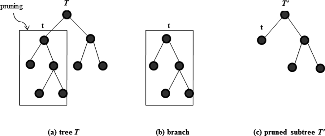
Illustration of pruning, branch, and subtree. The subtree is obtained by pruning the branch that roots from node t.

A subtree of the initial large tree T₀ will be selected as the final tree model. Nevertheless, the number of subtrees that a tree has increases very fast as the size of the tree or the number of terminal nodes grows. For example, a full tree of five depths, in which every terminal node has four ancestors, has 458,330 subtrees available. Thus, it is not computationally feasible to examine every possible subtree. The purpose of pruning is to narrow down the number of subtree choices by iteratively truncating the weakest link. In some ways, the pruning procedure resembles backward elimination in stepwise variable selection. The initial large tree plays the same role as the whole model that contains all structures and truncating an internal node amounts to removing one or more terms from the model. However, unlike backward elimination, there are no appropriate significance tests to determine when to stop the pruning process. Instead, pruning proceeds step-by-step to a natural end – the null tree model that contains the root node only. Specifics of the pruning algorithm are rather technical and beyond the scope of this introductory review. The result of pruning is a sequence of nested subtrees, T_M≺T_M−1≺···≺T₁≺T₀, where the symbol ≺ means is a subtree of and T_M is the null tree containing the root node only. Each subtree in the sequence enjoys certain optimality in terms of some tree performance criterion employed.

Finally, the best subtree is selected from this sequence via a separate cross-validation process. Two methods are available for this purpose, depending on the sample size. For large sample sizes, a section of the data set, called the validation sample, can be reserved for validating or reassessing the performance of T_M in the subtree sequence obtained from the pruning procedure. The subtree that performs best is then selected as the final tree, where the tree model performance can be measured by commonly used model selection criteria (Su, Wang, & Fan, 2004) such as Akaike (1974) Information Criterion (AIC) or Bayesian information criterion (BIC; Schwarz, 1978). If the sample available is moderately sized, resampling techniques such as v-fold cross validation or bootstrapping are used (see Breiman et al. (1984) and LeBlanc and Crowley (1993) for more in-depth discussions).

Merits of Trees

Major advantages of tree-based methods include the following. First, tree methods are nonparametric in nature and more robust to statistical assumptions. The tree implementations are made available in an automated manner and require less fitting efforts from the users. Tree methods are data-driven in the sense that the algorithm offers more freedom for the data to choose suitable basis functions (i.e., sets of indicator functions) that best approximate the true regression function. Second, easy and meaningful interpretations can be extracted by tracing the splitting rules down the path to each terminal node. These combined rules enable detection of what reason accounts for a low or high average outcome value. Third, categorical predictors are handled by defining dummy variables in linear models. The inclusion of many categorical predictors or categorical predictors with many levels may result in a massive model even before considering interactions among predictors. The tree method provides an efficient way to optimize the usage of categorical predictors in modeling by merging redundant levels. This feature is particularly attractive in nursing research studies where categorical variables commonly are collected. Fourth, trees are invariant to monotone transformations of predictors. For example, the binary question “ x ≤ c? “ for c > 0 induces exactly the same split on the data as “Is log(x) ≤ log(c)?” This property saves considerable fitting efforts in tree modeling. Fifth, the tree structure provides a natural and optimal way of grouping data, which renders tree methods attractive to many applications such as patient segmentation, subgroup analysis, disease prognosis or diagnosis, and risk scoring. Finally, trees excel in dealing with interactions of high order and substantial complexity. In linear regression, interaction terms are formulated commonly using cross-products. In practice, only first-order interactions are considered. Nevertheless, interactions may occur both in complex nonlinear forms and of higher orders. With the hierarchical tree architecture, complex interactions are handled implicitly yet thoroughly via tree analysis. In fact, the initial proposal of trees, Automatic Interaction Detection (AID) by Morgan and Sonquist (1963), was motivated by the problem of dealing with complex interactions among categorical variables in social surveys.

Limitations of Trees

Some limitations and remedial measures are noted for tree-structured methods. First, the tree method is unstable as an adaptive data-driven modeling tool in the sense that small perturbation in the data could lead to substantial changes in the final tree structure. Second, the piecewise-constant prediction function supplied by a tree model lacks continuity and smoothness and may not attain satisfactory accuracy in a predictive task. In particular, trees perform quite well in handling nonlinearity but they are less efficient in modeling linearity. It takes a relatively large tree structure to account for a linear pattern. There are additional limitations that are more inherent with tree methods. The greedy search scheme for best split achieves only local optimality for each node, but the resultant tree models are not necessarily globally optimal. In terms of variable selection, trees give preference to predictors that have more levels or values. Tree modeling is not recommended for samples that are of small sizes relative to the number of variables and the signal strength in the data.

A variety of tree extensions have been proposed in the literature to address or circumvent these above-mentioned limitations. Hastie, Tibshirani, and Friedman (2008) have described these extended tree methods that are among topics currently under intensive research in statistical science. In summary, as is the case with other research tools, nursing researchers should be aware of the advantages and disadvantages to apply tree methods appropriately.

Illustration of Tree-Structured Analysis Using Quality of Life Data

To illustrate the application of tree modeling, the Breast Cancer Education Intervention study (BCEI), a randomized quality of life (QOL) intervention trial with psychoeducational support for breast cancer survivors (BCSs) in their first year of posttreatment survivorship, was used. A detailed description of the BCEI and its efficacy assessment is described elsewhere (Meneses et al., 2007) and will be outlined briefly here.

The BCEI study was approved by the Institutional Review Boards of the university and participating cancer centers. Participants were recruited from a regional cancer center and private oncology offices in the southeastern United States. Inclusion criteria were: women at least 21 years of age with histologically confirmed Stage 0-II breast cancer, within 1 year of diagnosis, having at least 1 month time period since completion of surgery, having radiation therapy or chemotherapy to recover from acute treatment side effects, and willing and able to communicate in English. Exclusion criteria were advanced or metastatic disease at diagnosis. Women having hormonal therapy (aromatase inhibitor or tamoxifen) at study entry were not excluded. Two hundred and sixty-one (261) BCSs gave in-person written informed consent, and were assigned randomly to the experimental or wait control arm. The primary endpoint of the BCEI was overall QOL. Besides other measures, the following two sets of variables were collected in the study: (a) Breast Cancer Treatment and Socio-demographic Data Tool at baseline; and (b) the self-perceived QOL, measured at baseline, 3 months, and 6 months after study entry.

Breast Cancer Treatment and Sociodemographic Data Tool

This tool consists of 21 baseline variables used to document breast cancer treatment (i.e., surgery, radiation therapy, chemotherapy, hormonal, and anti-HER2 therapy) and sociodemographic characteristics (e.g., age, race, ethnicity, education, marital status, employment status, telephone and communication patterns, family income; Table 1).

Table 1.

Variable Description for the BCEI Data

	Variable Name	Type	Number of Levels or Values	Description
1	age	continuous	51	age at enrollment
2	race	binary	7	1 - Black/African American; 2 - Asian;
				3 - Caucasian; 4 - Hispanic/Latin; etc.
3	language	nominal	5	1 - English; 2 - Spanish; etc.
4	education	ordinal	5	education level: 1 - Grade school;
				2 - High school; etc.
5	religion	nominal	22	1 - Atheist; 2 - Buddhist; 3 - Catholic;
				4 - Christian; 5 - Jehovah Witness; etc.
6	marital	nominal	6	marital status: 1 - Never Married;
				2 - Married; 3 - Living with partner; etc.
7	family	nominal	14	family type: 1 - spouse; 2 - parents;
				3 - children; etc.
8	numfamily	count	7	number of family members
9	employment	nominal	4	1 - full time; 2 - part time;
				3 - retired; 0 - others.
10	income	ordinal	7	annual family income level: 1 - $10,000 or less;
				2 - $10,000-$20,000; 3 - $20,000-$30,000; etc.
11	other.cancer	binary	2	0 - none; 1 - yes
12	surgery	nominal	3	surgery type: 1 - lumpectomy;
				2 - mastectomy; 0 - others
13	chemotherapy	binary	2	0 - no; 1 - yes
14	radiotherapy	binary	2	0 - no; 1 - yes
15	rad.type	nominal	3	radiation type: 0 - none; 1 - primary;
				2 - postoperative.
16	hormonal	binary	2	0 - no; 1 - yes
17	type.horm	nominal	3	hormonal type: 0 - none; 1 - Tamoxifen; 2 - others
18	fatigue	binary	2	0 - no; 1 - yes
19	medfat	binary	2	any medicine for fatigue? 0 - no; 1 - yes
20	support	binary	2	currently with a breast cancer support group?
				0 - no; 1 - yes
21	nmth.diag	continuous	20	months since diagnosis

Quality of Life–Breast Cancer Survivors

The Quality of Life–Breast Cancer Survivors Scale (QOL-BC) is a 50-item scale measuring QOL in women with breast cancer (Ferrell, Dow, Leigh, Ly, & Gulasekaram, 1995) and was adapted from the QOL-Cancer Survivors Scale (Ferrell, Dow, & Grant, 1995). The QOL-BC uses a 10-point rating asking participants to describe overall QOL problems or concerns, and QOL concerns within four identified domains (physical, psychological, social, and spiritual well-being). A higher scale reflects more problems in QOL; a lower score indicates better QOL. The grand average of these 50 items is used as an overall measure of QOL. Test-retest reliability was 0.89 and Cronbach’s alpha for internal consistency was 0.93, reported in the original proposal of QOL-BC. In the present study, Cronbach’s alpha coefficient is 0.91 for overall QOL.

Of specific interest in this illustration is the relationship between baseline QOL and the predictor variables. For this purpose, linear regression is the conventional approach. The fitting results of the best linear model via stepwise selection are presented in Table 2. Three variables, age, chemotherapy, and number of months since diagnosis are retained in the final model, which yields a R² of 0.194. The estimated slope parameters can be interpreted in the following ways – either at the individual level or at the population level. Given two BCSs (e.g., A and B) who have the same chemotherapy status and same number of months since diagnosis, the QOL score reported by participant A is expected to be 0.3 (± 0.07) less (reflecting better QOL) than participant B if participant A is 10 years older. With same age and number of months since diagnosis, BCSs who received chemotherapy have a 0.449 (± 0.184) higher QOL score compared with those who have not received chemotherapy.

Table 2.

Multiple Linear Regression Model vs. the Final Tree Model for Baseline QOL in the BCEI Data

Model Type	Predictor	Parameter Estimate	Standard Error	t-test	Two- Sided p-value
Linear regression	intercept	4.203	0.474	8.870	< .0001
	age	−0.030	0.007	−4.127	< .0001
	chemotherapy	0.449	0.184	2.433	.0156
	nmth.diag	0.052	0.025	2.096	.0370
	df = 257; R2 = 19.40%; AIC = 829.126; BIC = 846.949
Tree	intercept	3.099	0.149	20.785	< .0001
	node-III	−0.627	0.216	−2.899	.0010
	node-I	0.644	0.179	3.592	< .0001
	df = 258; R2 = 17.39%; AIC = 833.558; BIC = 847.816

Notes. Obtained via stepwise selection.

Next, a tree analysis was performed using R software. A large initial tree with 19 terminal nodes was first constructed with relaxed stopping rules. It represents a highly complex model with many terms. The pruning algorithm yielded a sequence of 18 nested subtrees. Due to the moderate sample size, 10-fold cross-validation was used to aid in the tree size determination. The cross-validated deviance versus tree size is plotted in Figure 4. The AIC and BIC were computed accordingly and added to the plot. The best tree sizes were 3, 3, and 2, supplied by the minimum values of cross-validated deviance, AIC, and BIC, respectively; the one with three terminal nodes is further explored as the final tree structure.

Figure 4.

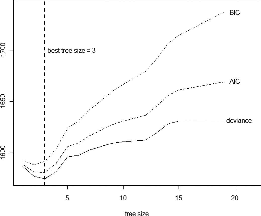
Tree size determination for baseline QOL data via 10-fold cross-validation. A tree model with a smaller AIC or BIC is preferred.

The tree diagram is plotted in Figure 5. The data set was first split into younger and older BCSs with the cutoff age of 60 years. The older group (Node III) contained 68 BCSs with an average QOL score of 2.472. The younger group (< 60 years of age) consisted of 188 BCSs and were further split according to whether they had completed chemotherapy treatment. The 126 younger BCSs who had received chemotherapy (Node I) were associated with the worst QOL, reporting the highest average QOL score of 3.743. The other 62 younger BCS (Node II) who had not received chemotherapy had an average QOL score of 3.099.

Figure 5.

The final decision tree structure for baseline QOL. Given in each terminal node are the node size (i.e., number of BCSs) and the average QOL score.

Additional graphical exploration of these three groups identified by the tree model is provided in Figure 6. Specifically, Figure 6(a) plots the original QOL scores versus age, which shows a threshold effect at age 60 years. The chemotherapy status is indicated among younger BCSs in the plot. Figure 6(b) provides the parallel boxplots (also called five-number summary plots) for comparison. The QOL scores in three terminal nodes all are distributed roughly normally with similar variations. The tree model can be rewritten in a linear model form with dummy variables. The resultant model fit is presented in Table 2(b). With a simple structure, the tree model provides a rather comparable fitting performance to the best linear model. Furthermore, the grouping rules identified in the tree structure could be applied to future strategic research on planning interventions. The tree structure suggests that future interventions may be particularly beneficial to subjects in Node I; that is, younger BCSs who received chemotherapy. These BCSs are associated with the highest average QOL or the worst QOL score and hence have more room for improvement with tailored interventions.

Figure 6.

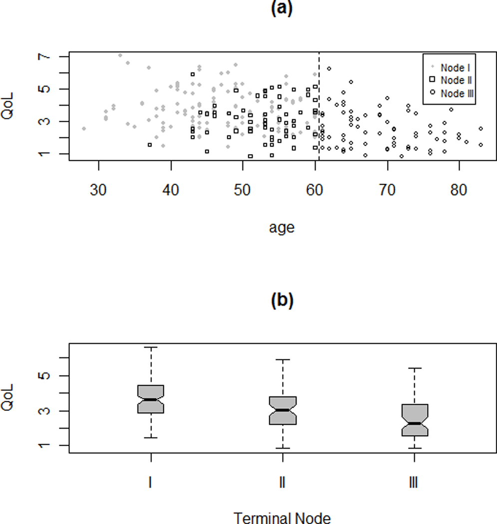
Two plots for exploring the three terminal nodes (I, II, and III) in the final tree: (a) plot of QOL versus Age with threshold at 60, the status of whether the patient took drug for cancer treatment also symbolized among younger patients; and (b) parallel box-plots. Node I contains younger BCSs who were no older than 60 years and had received chemotherapy; Node II contains younger BCSs who were no older than 60 years and did not have chemotherapy; and Node III contains older individuals of age above 60 years.

Two variables are involved in the tree splitting, age and chemo. Variables present in the final tree structure can be deemed as important. On the other hand, variables not showing up in tree splitting are not necessarily unimportant ones since their effects might have been masked by other correlated ones (Breiman et al., 1984). This masking effect is analagous to the confounding effect in linear regression. The goal is to identify which varaibles are important for predicting QOL. This question can be better answered using the variable importance ranking feature supplied in random forests (RF; Breiman, 2001), one of the tree extentions. In this approach, a forest is formed by constructing a large numer of tree models with bootstrap resampling. For each tree, the predictive power of every variable is assessed via permutation. The information is then integrated across the forest of trees to provide an overall evaluation of importance of each predictor in predicting the response. The resultant variable importance measures for BCEI data are plotted in Figure 7. Age is identified as the most important varaible in determining QOL, followed by number of months since diagnosis, chemotherapy status, number of family members, and employment status.

Figure 7.

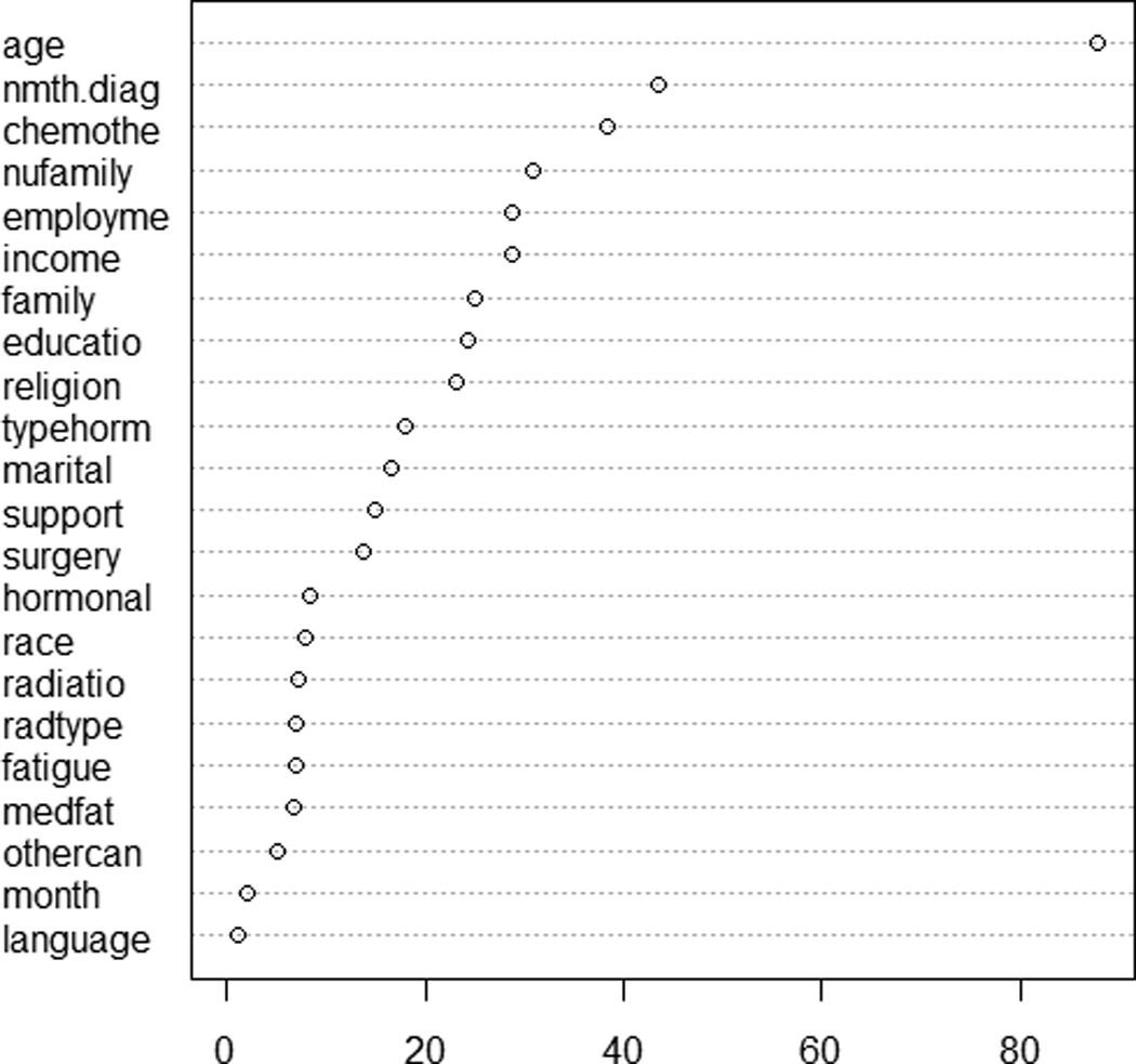
Variable importance ranking for baseline QOL computed from random forests (RF). The RF options include 5,000 trees constructed with bootstrap samples and six predictors randomly selected at each node. The horizontal axis stands for the increased node purity.

Discussion

In the example, the tree analysis was contrasted with linear regression to better illustrate their advantages and limitations. Tree methods take a very different approach than traditional linear regression, offering new insights to statistical modeling. It is important to note the different ways of making interpretations between the two methods. Interpretation of linear regression is made via conventional statistical inference (i.e., confidence intervals or significance testing). Often, only the predictors included in the final linear model are deemed as important and further discussed. Comparatively, tree models are built on cross-validation and interpretation is extracted from the decision rules. Although similar t-test results are presented in Table 2(b) for the tree model, their associated p-values are overoptimistic because of the adaptive nature of recursive partitioning and therefore should not be cited. The variable importance ranking feature in RF offers excellent complementary information to the single tree analysis. It faciliates a comprehensive assessment of the importance of each predictor under the joint influence of other predictors.

Often obtaining a best linear model takes tremendous fitting efforts, calling for techniques ranging from level collapsing and dummy variables for categorical predictors, variable selection, and interaction detection, to residual analysis, variable transformation, and other model diagnostics, requiring considerable time and effort from a sophisticated analyst. On the other hand, despite the complexity and intensity of computation, tree modeling is data-driven and automated by computer algorithms, requiring little interactive input during its fitting process.

Looking at the final tree structure in Figure 5, it is not clear whether or not getting chemotherapy made a difference in QOL in the older age group (Node III). This question also has to do with whether an interaction exists between age and chemotherapy in terms of their effects on QOL. The results show that older BCSs were less likely to receive chemotherapy compared with younger BCSs. Out of 194 younger BCSs, 132 received chemotherapy, while out of 70 older BCSs, only 12 received chemotherapy. Perhaps because of the small sample size in Node III, no further split on chemotherapy shows up in the final tree structure. For this reason, it is difficult to fully address the issue with the BCEI data set. In general, the structure found with Node I and Node II should not be interpreted necessarily as interaction between age and chemotherapy. Interactions are handled implicitly by tree modeling and it takes further research efforts to understand which variables interact with which for a given tree structure. See Su, Tsai, Wang, Nickerson, and Li (2009) for a discussion on how to explicitly extract treatment-by-covariate interactions with tree methods.

Implications for Nursing Research

As technological capacity increases, there is a concomitant exponential increase in activity and data to fill the expanded capacity. This adage seems true when considering nursing research. Data encountered by nurse researchers and interdisciplinary teams have been growing both in size and in complexity. It is critical to be aware of the methodological obstacles and issues in dealing with huge complex datasets. For example, a common predicament with statistical testing is that nearly every variable, even those with practically negligible effects, become statistically significant merely because of a large sample size. The challenges posed by huge data sets have led to a new emerging field, data mining. Using internally built-in cross validation rather than statistical testing, tree-based methods, together with the various extensions, constitute a fundamental family of analytic tools in data mining. Tree methods offer an attractive alternative for analyzing complex data and generate new findings that may not be uncovered using traditional modeling approaches.

Tree models also can play a critical role in nursing informatics, which is aimed at facilitating the integration of data, information, and knowledge to support patients, nurses, and other care providers in their decision-making in all roles and settings. Unlike other modeling tools, the collection of meaningful splitting rules produced by trees can be useful in developing model-based decision support systems for intervention and care planning.

References

- Adak S. Time-dependent spectral analysis of non-stationary time series. Journal of the American Statistical Association. 1998;93(444):1488–1501. [Google Scholar]
- Akaike H. A new look at the statistical model identification. IEEE Transactions an Automatic Control. 1974;19(6):716–723. [Google Scholar]
- Breiman L. Random forests. Machine Learning. 2001;45(1):5–32. [Google Scholar]
- Breiman L, Friedman J, Olshen R, Stone C. Classification and regression trees. Belmont, CA: Wadsworth International Group; 1984. [Google Scholar]
- Cho S-H, Ketefian S, Barkauskas VH, Smith DG. The effects of nurse staffing on adverse events, morbidity, mortality, and medical costs. Nursing Research. 2003;52(2):71–79. doi: 10.1097/00006199-200303000-00003. [DOI] [PubMed] [Google Scholar]
- Choi Y, Ahn H, Chen JJ. Regression trees for analysis of count data with extra Poisson variation. Computational Statistics and Data Analysis. 2005;49(3):893–915. [Google Scholar]
- Crichton NJ, Hinde JP, Marchini J. Models for diagnosing chest pain: Is CART helpful? Statistics in Medicine. 1997;16(7):717–727. doi: 10.1002/(sici)1097-0258(19970415)16:7<717::aid-sim504>3.0.co;2-e. [DOI] [PubMed] [Google Scholar]
- Duffy ME. Methodological issues in web-based research. Journal of Nursing Scholarship. 2002;34(1):83–88. doi: 10.1111/j.1547-5069.2002.00083.x. [DOI] [PubMed] [Google Scholar]
- Fan J, Su XG, Levine RA, Nunn ME, LeBlanc M. Trees for correlated survival data by goodness of split, with applications to tooth prognosis. Journal of the American Statistical Association. 2006;101(475):959–967. [Google Scholar]
- Ferrell BR, Dow KH, Grant M. Measurement of the quality of life of cancer survivors. Quality of Life Research. 1995;4(6):523–531. doi: 10.1007/BF00634747. [DOI] [PubMed] [Google Scholar]
- Ferrell BR, Dow KH, Leigh S, Ly J, Gulasekaram P. Quality of life in long-term cancer survivors. Oncology Nursing Forum. 1995;22(6):915–922. [PubMed] [Google Scholar]
- Hastie T, Tibshirani R, Friedman JH. Elements of statistical learning. 2nd ed. New York, NY: Chapman and Hall; 2008. [Google Scholar]
- Henry SB. Nursing informatics: State of the science. Journal of Advanced Nursing. 1995;22(6):1182–1192. doi: 10.1111/j.1365-2648.1995.tb03121.x. [DOI] [PubMed] [Google Scholar]
- Hess KR, Abbruzzese MC, Lenzi R, Raber MN, Abbruzzese JL. Classification and regression tree analysis of 1000 consecutive patients with unknown primary carcinoma. Clinical Cancer Research. 1999;5(11):3403–3410. [PubMed] [Google Scholar]
- Kass GV. An exploratory technique for investigating large quantities of categorical data. Applied Statistics. 1980;29:119–127. [Google Scholar]
- Lange LL, Jacox A. Using large data bases in nursing and health policy research. Journal of Professional Nursing. 2004;9(4):204–211. doi: 10.1016/8755-7223(93)90037-d. [DOI] [PubMed] [Google Scholar]
- LeBlanc M, Crowley J. Survival trees by goodness of split. Journal of the American Statistical Association. 1993;88(422):457–467. [Google Scholar]
- Lee S-K. On generalized multivariate decision tree by using GEE. Computational Statistics & Data Analysis. 2005;49(4):1105–1119. [Google Scholar]
- Lee S-K, Jin S. Decision tree approaches for zero-inflated count data. Journal of Applied Statistics. 2006;33(8):853–865. [Google Scholar]
- Mair J, Smidt J, Lechleitner P, Dienstl F, Puschendorf B. A decision tree for the early diagnosis of acute myocardial infarction in nontraumatic chest pain patients at hospital admission. Chest. 1995;108(6):1502–1509. doi: 10.1378/chest.108.6.1502. [DOI] [PubMed] [Google Scholar]
- McKenzie DP, McGorry PD, Wallace CS, Low LH, Copolov DL, Singh BS. Constructing a minimal diagnostic decision tree. Methods of Information in Medicine. 1993;32(2):161–166. [PubMed] [Google Scholar]
- Meneses KD, McNees P, Loerzel VW, Su X, Zhang Y, Hassey LA. Transition from treatment to survivorship: effects of a psychoeducational intervention on quality of life in breast cancer survivors. Oncology Nursing Forum. 2007;34(5):1007–1016. doi: 10.1188/07.ONF.1007-1016. [DOI] [PubMed] [Google Scholar]
- Morgan J, Sonquist J. Problems in the analysis of survey data and a proposal. Journal of the American Statistical Association. 1963;58(302):415–434. [Google Scholar]
- Quinlan JR. C4.5: Programs for machine learning. San Francisco, CA: Morgan Kaufmann Publishers Inc; 1993. [Google Scholar]
- R Development Core Team. R: A language and environment for statistical computing. Vienna, Austria: R Foundation for Statistical Computing; 2010. [Google Scholar]
- Schwarz G. Estimating the dimension of a model. The Annals of Statistics. 1978;6(2):461–464. [Google Scholar]
- Segal MR. Tree-structured methods for longitudinal data. Journal of the American Statistical Association. 1992;87(418):407–418. [Google Scholar]
- Steffann J, Feyereisen E, Kerbrat V, Romana S, Frydman N. Prenatal and preimplantation genetic diagnosis: Decision tree, new practices? (French) Medicine Sciences. 2005;21(11):987–992. doi: 10.1051/medsci/20052111987. [DOI] [PubMed] [Google Scholar]
- Su XG, Tsai C-L, Wang H, Nickerson D, Li B. Tree-based subgroup analysis via recursive partitioning. Journal of Machine Learning Research. 2009;10:141–158. [Google Scholar]
- Su XG, Wang M, Fan JJ. Maximum likelihood regression trees. Journal of Computational and Graphic Statistics. 2004;13(3):586–598. [Google Scholar]
- Vlahou A, Schorge JO, Gregory BW, Coleman RL. Diagnosis of ovarian cancer using decision tree classification of mass spectral data. Journal of Biomedicine & Biotechnology. 2003;5:308–314. doi: 10.1155/S1110724303210032. [DOI] [PMC free article] [PubMed] [Google Scholar]