TWO-STAGE EMPIRICAL LIKELIHOOD FOR LONGITUDINAL NEUROIMAGING DATA ^*

Abstract

Longitudinal imaging studies are essential to understanding the neural development of neuropsychiatric disorders, substance use disorders, and the normal brain. The main objective of this paper is to develop a two-stage adjusted exponentially tilted empirical likelihood (TAETEL) for the spatial analysis of neuroimaging data from longitudinal studies. The TAETEL method allows us to efficiently analyze longitudinal data without correctly modeling temporal correlation and to classify different time-dependent covariate types. To account for spatial dependence, the TAETEL method developed here specifically combines all the data in the neighborhood of each voxel (or pixel) on a 3 dimensional (3D) volume (or 2D surface) with appropriate weights to calculate adaptive parameter estimates and adaptive test statistics. Simulation studies are used to examine the finite sample performance of the adjusted exponential tilted likelihood ratio statistic and TAETEL. We demonstrate the application of our statistical methods to the detection of the difference in the morphological changes of the hippocampus across time between schizophrenia patients and healthy subjects in a longitudinal schizophrenia study.

1. Introduction

Neuroimaging data, including both anatomical and functional magnetic resonance imaging (MRI), have been/are being widely collected to understand the neural development of neuropsychiatric disorders, substance use disorders, and the normal brain in various longitudinal studies [Almli et al. (2007)]. For instance, various morphometrical measures of the morphology of the cortical and subcortical structures (e.g., hippocampus) are extracted from anatomical MRIs for understanding neuroanatomical differences in brain structure across different populations and across time. Studies of brain morphology have been conducted widely to characterize differences in brain structure across groups of healthy individuals and persons with various diseases, and across time [Thompson and Toga (2002), Thompson et al. (2002), Styner et al. (2005), Zhu et al. (2008)]. Moreover, functional MRI (fMRI) is a valuable tool for understanding functional integration of different brain regions in response to specific stimuli and behavioral tasks and detecting the association between brain function and covariates of interest, such as diagnosis, behavioral task, severity of disease, age, or IQ [Friston (2007), Rogers et al. (2007), Huettel et al. (2004)].

Much effort has been devoted to developing frequentist and Bayesian methods for analyzing neuroimaging data using numerical simulations and theoretical reasoning. Frequentist statistical methods for analyzing neuroimaging data are often sequentially executed in two steps. The first step involves fitting a general linear model or a linear mixed model to neuroimaging data from all subjects at each voxel [Beckmann, Jenkinson, and Smith (2003), Friston et al. (2005), Rowe (2005), Woolrich et al. (2004), Zhu et al. (2008)]. The second step is to calculate adjusted p-values that account for testing the hypotheses across multiple brain regions or across many voxels of the imaging volume using various statistical methods (e.g., random field theory, false discovery rate, or permutation method) [Cao and Worsley (2001), Friston et al. (1996), Hayasaka and Nichols (2004), Logan and Rowe (2004), Worsley et al. (2004)]. Most of these frequentist methods have been implemented in existing neuroimaging software platforms including SPM and FSL, among many others. In the recent literature, a number of papers have been published on the development of spatial-temporal models for functional imaging data using a Bayesian approach [Penny et al. (2007), Bowman et al. (2008), Woolrich et al. (2004), Luo and Puthusserypady (2005)]. Most Bayesian approaches, however, are less practical due to the extensive computational burden of running Markov chain Monte Carlo sampling in a large number of voxels, and thus they are limited to small or moderate anatomic regions and a small number of regions of interest (ROI) [Bowman et al. (2008)]. Moreover, as discussed in Snook et al. (2007), the major drawbacks of ROI analysis include the instability of statistical results obtained from ROI analysis and the partial volume effect in relatively large ROIs.

Existing statistical methods in the neuroimaging literature have two major limitations for analyzing longitudinal neuroimaging data, as explained below. The respective strategies to resolve these two limitations are detailed in Section 2. The first limitation is that the parametric models including linear mixed models as discussed above require the correct specification of the temporal correlation structure and cannot properly distinguish between different types of time-dependent covariates (types I, II, and III) [Lai and Small (2007), Pepe and Anderson (1994)]. A distinctive feature of longitudinal neuroimaging data is its ability to characterize individual changes in neuroimaging measurements (e.g., volumetric and morphometric) over time. Imaging measurements on the same individual usually exhibit positive correlation and the strength of the correlation decreases with time separation [Liang and Zeger (1996)]. Moreover, longitudinal data may provide crucial information for a causal role of time-dependent covariates (e.g., exposure) in disease processes [Diggle et al. (2002), Lai and Small (2007), Pepe and Anderson (1994)]. Improperly handling the time-dependent covariates and ignoring (or incorrectly modeling) the temporal correlation structure in imaging measures would likely influence the subsequent statistical inference, such as increasing the false positive and negative rates and thus yield misleading scientific inference [Diggle et al. (2002), Lai and Small (2007)].

The second limitation is that most smoothing methods apply the same amount of smoothing throughout the whole image, which can be problematic near the edges of the activated regions. Although it is common to apply a smoothing step before applying a voxel-wise approach for the analysis of neuroimaging data [Poline and Mazoyer (1994), Shafie et al. (2003), Lindquist and Wager (2008)], the voxel-wise method suffers from the same amount of smoothing throughout the whole image and the arbitrary choice of smoothing extent [Hecke et al. (2009), Jones et al. (2005)]. Jones et al. (2005) have shown that the final results of a voxel-based analysis can strongly depend on the amount of smoothing in the smoothed diffusion imaging data. Recently, Yue, Loh and Lindquist (2010) introduce a spatially smoothing method using nonstationary spatial Gaussian Markov random fields to spatially and adaptively smooth images. Their approach, however, can be computationally intensive for 3D imaging data.

In this paper, we develop new statistical methods to resolve these two limitations. To resolve the first limitation, we develop an adjusted empirical likelihood method, called AETEL, for the analysis of longitudinal neuroimaging data with time-dependent covariates. AETEL, as a nonparametric method, is built on a set of estimating equations and the number of estimating equations can be larger than the number of parameters. Thus, it avoids parametric assumptions and this feature is very appealing for the analysis of real neuroimaging data, such as brain morphological measures, since the distribution of the univariate (or multivariate) neuroimaging measurements often deviates from the Gaussian distribution [Ashburner and Friston (2000), Salmond et al. (2002), Luo and Nichols (2003)]. Using more estimating equations than the number of parameters allows us to appropriately handle time-dependent covariates of different types and to make an efficient use of the estimating equations without the need of correctly modeling the temporal correlation in longitudinal data [Lai and Small (2007), Qu et al. (2000)]. AETEL also provides a natural test statistic to test whether a specific covariate is of a certain type (types I, II, and III).

To resolve the second limitation, we develop a two-stage AETEL, abbreviated as TAETEL, for the analysis of longitudinal neuroimaging data. TAETEL integrate a smoothing method into our AETEL for carrying out statistical inference on neuroimaging data. The TAETEL method, as an adaptive procedure, fits AETEL at each voxel in stage 1. Then, TAETEL uses the information learned from stage 1 to discard the data from the neighboring voxels with dissimilar signal pattern and to incorporate the data from the neighboring voxels with similar signal pattern to adaptively calculate parameter estimates and test statistics. TAETEL allows the amount of smoothing to adapt to the spatial extent of activation, and thus it avoids using the same amount of smoothing throughout the whole image as in most smoothing methods. In addition, theoretically, we can establish asymptotic consistency and normality of the estimators and test statistics obtained from TAETEL.

Section 2 of this paper introduce the shape data of the hippocampus structure from a longitudinal schizophrenia study and presents the new statistical methods just described. In Section 3, we conduct simulation studies to examine the finite sample performance of the TAETEL method. Section 4 illustrates an application of the proposed methods to the longitudinal schizophrenia study of the hippocampus. We present some concluding remarks in Section 5.

2. Data and methods

2.1. Longitudinal schizophrenia study of hippocampus shape

This is a longitudinal, randomized, controlled, multisite, double-blind study conducted at 14 academic medical centers in North America and western Europe, with partial funding from Lilly Research Laboratories [Lieberman et al. (2005), Styner et al. (2004)]. In this study, 238 first-episode schizophrenia patients were enrolled meeting the following criteria: age 16 to 40 years; onset of psychiatric symptoms before age 35; diagnosis of schizophrenia, schizophreniform, or schizoaffective disorder according to DSM-IV criteria; and various treatment and substance dependence conditions. After random allocation at baseline, 123 patients were selected to receive a conventional antipsychotic, haloperidol (2–20 mg/d), and 115 were selected to receive an atypical antipsychotic olanzapine (5–20 mg/d). Patients were treated and followed up to 47 months. Also, 56 healthy control subjects matched to the patient’s demographic characteristics were also enrolled. Neurocognitive and MRI assessments were performed at approximately months 0 (baseline), 3, 6, 13, 24, 36 and 47 with different subjects having different visiting times, and some subjects dropped out during the course of the study.

The hippocampus, a gray matter structure in the limbic system, is involved in processes of motivation and emotions and has a central role in the formation of memory. The hippocampus is a paired structure with mirror-image halves in the left and right brain hemisphere and located inside the medial temporal lobe (Figure 1). Many MRI studies have reported the reduction of hippocampal volume in schizophrenia subjects and at onset of the first episode of psychotic symptoms before effects associated with treatment and disease chronicity [Lieberman et al. (2005)].

Fig 1.

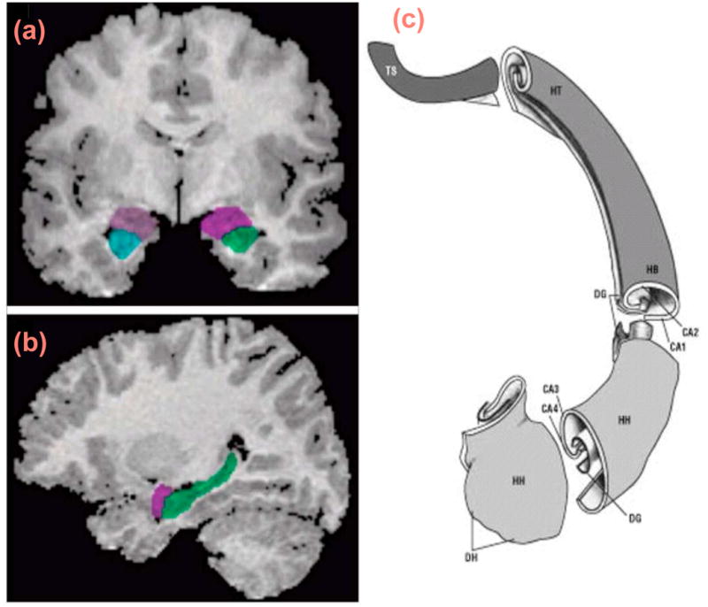
Location of hippocampus colored in green in the context of the surrounding structures in the coronal (a) and sagittal (b) views. Subregions of the hippocampus in (c) showing the head of the hippocampus (HH), the digitationes hippocampi (DH), the hippocampal body (HB), the hippocampal tail (HT), the terminal segment of the HT (TS), the dentate gyrus (DG), and the fields of the cornu ammonis (CA1–CA4). Adapted with permission from Springer Verlag, Heidelberg, Germany [Duvernoy (2005)].

The aim of this study is to use the boundary and medial shape of the left and right hippocampi to examine whether hippocampal abnormalities are present in schizeophrenic patients. Statistical shape modeling and analysis have emerged as important tools for understanding cortical and subcortical structures from medical images [Dryden and Mardia (1998)]. We consider two approaches for shape representation including a parametric boundary description called SPHARM and a medial shape description [Pizer et al. (2003), Styner and Gerig (2003)]. The SPHARM can only represent objects of spherical topology, while the medial representation provides information on a rich set of features including local thickness. These shape features are not accessible by conventional volume-based morphometry and offer a great opportunity to address the weaknesses of conventional volumetric methods.

We consider two sets of responses of interest. The first set of responses was based on the SPHARM representation of hippocampal surfaces. We use the SPHARM-PDM [Styner et al. (2004)] shape representation to establish surface correspondence and align the surface location vectors across all subjects. The sampled SPHARM-PDM is a smooth, accurate, fine-scale shape representation. The hippocampal surfaces of different subjects are thus represented by the same number of location vectors (with each location vector consisting of the spatial x, y, and z coordinates of the corresponding vertex on the SPHARM-PDM surface) and are used as the first set of responses. Some covariates of interest include race (Caucasian, African American and others), age (in years), gender, group (the schizophrenia group and the healthy control group) and time (visiting in weeks).

The second set of responses was the hippocampus m-rep thickness at the 24 medial atoms of the left and the right brain (Figure 4). The m-rep is a linked set of medial primitives named medial atoms, which are formed from two equal length vectors and are composed of a position, a radius, a frame implying the tangent plane to the medial manifold and an object angle [Styner et al. (2004)]. The m-rep thickness is the radius of each medial atom and provides moderate local feature compared with volume size. Covariates of interest were Whole Brain Volume (WBV), race (Caucasian, African American and others), age (in years), gender, diagnostic status (patient or control) and visit times (in weeks). This WBV measure includes gray and white matter, ventricular cerebrospinal fluid, cisterns, fissures, and cortical sulci. The WBV is commonly used as a covariate in statistical analyses to control for scaling effects [Arndt et al. (1991)]. Particularly, WBV is a time-dependent covariate and may vary with the hippocampus thickness measurement.

Fig 4.

M-rep representation of hippocampal structures: (a) an m-rep model of the hippocampus; (b) the boundary surface of the m-rep model of hippocampus; (d) m-rep radius (or thickness) measures at the five atoms from two m-rep objects; (c) shows the −log₁₀(p)-values for the Shapiro-Wilk test for the residuals at each atom on the left hippocampus; (e) shows the −log₁₀(p)-values for the Shapiro-Wilk test for the residuals at each atom on the right hippocampus. The red horizontal line is the −log₁₀(0.05) cut-off line.

2.2. Estimating equations for longitudinal data

We consider a longitudinal study of imaging data with n subjects, where a q × 1 covariate x_i,j (e.g., age, gender, height and brain volume) is obtained for the ith subject at the j-th time point t_ij for i = 1, ···, n and j = 1, ···, m_i. Without loss of generality, we assume that t_i1 < ···< t_imi for all i. Thus, there are at least ${\sum }_{i=1}^n{m}_i=N$ images in the study. Based on each image, we observe or compute neuroimaging measures, denoted by Y_i = {y_ij(d): d ∈ , j = 1, ···, m_i}, across all m_i time points from the ith subject, where d represents a voxel (or atom, or point) on , a specific brain region of a normalized brain. The imaging measure y_ij(d) at each voxel d can be either univariate or multivariate. For example, the m-rep thickness is a univariate measure, whereas the location vector of SPHARM is a three dimensional MRI measure at each point [Styner and Gerig (2003), Chung et al. (2007)]. For notational simplicity, we assume that the y_ij(d) are univariate measures.

We temporarily drop voxel d from our notation. At a specific voxel d in the brain region, the z_i = {(y_ij, x_ij): j = 1, ···, m_i} are independent and satisfy a moment condition

$$E\{g({\mathbf{z}}_i,\theta )\}=0,\text{for}i=1,\cdots ,n,$$ (2.1)

where θ is a p×1 vector, g(·, ·) is an r×1 vector of known functions with r ≥ p and E denotes the expectation with respect to the true distribution of all z_i’s. Equation (2.1) is often referred to as a set of unbiased estimating equations or moments model [Qin and Lawless (1994), Hansen (1982)]. The moments model (2.1) is more general than most parametric models including linear mixed models, which are often used for the analysis of neuroimaging data [Worsley et al. (2004), Qin and Lawless (1994), Hansen (1982), Schennach (2007), Owen (2001), Diggle et al. (2002)].

For longitudinal data, although the measurements from different subjects are independent, measurements within the same subject may be highly correlated. The generalized estimating equations (GEE) assume a working covariance matrix for y_i = (y_i1, ···, y_imi)^T given by V_i. Let E(y_i) = μ_i(β) = (μ_i1(β), ···, μ_imi (β))^T and D_i(β) = ∂μ_i(β)/∂β. Under the assumption that $E\{D_i{(\beta )}^T{V}_i^{-1}[{\mathbf{y}}_i-{\mu }_i(\beta )]\}=0$, Liang and Zeger (1986) proposed an estimator, denoted by β̂_gee, which solves a set of GEEs as follows:

$$G(\beta )=\sum _{i=1}^n{D}_i{(\beta )}^T{V}_i^{-1}[{\mathbf{y}}_i-{\mu }_i(\beta )]=\mathbf{0}.$$ (2.2)

For longitudinal data with time-dependent covariates, whether $g({\mathbf{z}}_i,\theta )=E\{D_i{(\beta )}^T{V}_i^{-1}[{\mathbf{y}}_i-{\mu }_i(\beta )]\}$ equals zero or not depends on the type of time-dependent covariates and the structure of V_i [Lai and Small (2007)]. The time-dependent covariate x_ij is of type I if

$$E\{{\partial }_{\beta }{\mu }_{is}(\beta )[{\mathbf{y}}_{ij}-{\mu }_{ij}(\beta )]\}=0\text{for}\text{all}s,j=1,\cdots ,m_i,$$ (2.3)

where ∂_β = ∂/∂β. A sufficient condition for type I covariates is E[y_ij|x_ij] = E[y_ij|x_i1, ···, x_imi]. For type I covariates, we can set $g({\mathbf{z}}_i,\theta )=D_i{(\beta )}^T{V}_i^{-1}[{\mathbf{y}}_i-{\mu }_i(\beta )]$ and show that E[g(z_i, θ)] = 0. If V_i is the true covariance matrix of y_i, then the estimator β̂_gee is an efficient estimator. However, β̂_gee is inefficient under a misspecified V_i. To increase the efficiency, we may choose several candidate working covariance matrices $M_i^{(1)},\cdots ,M_i^{(s_0)}$ and assume $V_i^{-1}={\sum }_{k=1}^{s_0}{\alpha }_k{M}_i^{(k)}$ for some unknown constants α_k [Qu et al. (2000)]. Then, following Qu et al. (2000), we consider a set of estimating equations given by

$$g({\mathbf{z}}_i,\theta )=\left(\begin{array}{c}{D}_i{(\beta )}^T{M}_i^{(1)}[{\mathbf{y}}_i-{\mu }_i(\beta )]\\ ⋮\\ D_i{(\beta )}^T{M}_i^{(s_0)}[{\mathbf{y}}_i-{\mu }_i(\beta )]\end{array}\right)\text{for}i=1,\cdots ,n.$$ (2.4)

In this case, the number of functions in g(z_i, θ) is s₀q > q, when s₀ > 1.

The time-dependent covariate x_ij is of type II if

$$E\{{\partial }_{\beta }{\mu }_{is}(\beta )[{\mathbf{y}}_{ij}-{\mu }_{ij}(\beta )]\}=0\text{for}\text{all}s\ge j,j=1,\cdots ,m_i.$$ (2.5)

A sufficient condition for type II covariates is

$$p({\mathbf{x}}_{i,t+1},\cdots ,{\mathbf{x}}_{{im}_i}\mid {\mathbf{y}}_{it,}{\mathbf{x}}_{it})=p({\mathbf{x}}_{i,t+1},\cdots ,{\mathbf{x}}_{{im}_i}\mid {\mathbf{x}}_{it}).$$ (2.6)

For type II covariates, we can set g(z_i, θ) = D_i(β)^T [y_i − μ_i(β)], in which an independent working covariance matrix is used. However, the estimator β̂_gee based on the independent working correlation matrix is inefficient, since we do not use the information contained in E{∂_βμ_is(β)[y_ij − μ_ij(β)]} = 0 for all s > j. To increase the efficiency of the estimate, we choose a set of lower triangular matrices $L_i^{(1)},\cdots ,L_i^{(s_0)}$, and then we consider the estimating equations given by

$$g({\mathbf{z}}_i,\theta )=\left(\begin{array}{c}{D}_i{(\beta )}^T{L}_i^{(1)}[{\mathbf{y}}_i-{\mu }_i(\beta )]\\ ⋮\\ D_i{(\beta )}^T{L}_i^{(s_0)}[{\mathbf{y}}_i-{\mu }_i(\beta )]\end{array}\right)\text{for}i=1,\cdots ,n.$$ (2.7)

In this case, the number of functions in g(z_i, θ) is s₀q > q, when s₀ > 1. Suppose that m₁ = ···= m_n. We can set s₀ = m₁(m₁+1)/2 and $L_i^{(b)}={\mathbf{e}}_s{\mathbf{e}}_j$, where e_s is a q×1 vector with sth component 1 and 0 otherwise. Thus, similar to Lai and Small (2007), we are able to pick ∂_βμ_is(β)[y_ij − μ_ij(β)] for all s ≥ j.

The time-dependent covariate x_ij is of type III if

$$E\{{\partial }_{\beta }{\mu }_{is}(\beta )[{\mathbf{y}}_{ij}-{\mu }_{ij}(\beta )]\}\ne 0\text{for}\text{some}s>j.$$ (2.8)

For type III covariates, we need to choose V_i as a diagonal matrix. For instance, if V_i = I_mi, where I_mi is an m_i × m_i identity matrix, then g(z_i, θ) = D_i(β)^T [y_i − μ_i(β)]. Furthermore, if we assume a specific form for the variances for all y_ij, then we may set V_i = diag(Cov(y_i)).

An overall strategy for analyzing models with time-dependent covariates is to first assume that the time-dependent covariates are of type III. Then we test whether the time-dependent covariates are of type II, and if the test is not rejected, we can go on to test if they are of type I. Once the type of all the time-dependent covariates is decided, we use the corresponding estimating equations. See section 4 for more details.

2.3. Adjusted exponentially tilted empirical likelihood

We consider a non-parametric method, called exponentially titled empirical likelihood, to carry out statistical inference about θ based on a set of estimating equations {g(z_i, θ): i = 1, ···, n} [Schennach (2007)]. The exponentially titled empirical likelihood (ETEL) method is a combination of the empirical likelihood and the exponentially tilted method. Statistically, ETEL improves several alternative methods for estimating equations, including empirical likelihood (EL), exponentially tilted likelihood, generalized estimating equations (GEE), and generalized method of moments (GMM), both empirically and theoretically [Schennach (2007)]. However, most empirical likelihood methods including ETEL suffer from two pitfalls: low precision of the chi-square approximation and non-existence of solutions to the estimating equations [Chen et al. (2008), Liu and Chen (2010)]. Chen et al. (2008) introduce a novel adjustment to these empirical likelihood methods and develop an iterative algorithm that converges very fast. Simulation studies have shown that the adjusted empirical likelihood methods perform as well as the linear regression model with Gaussian noise when data are symmetrically distributed, while the adjusted empirical likelihood methods are superior when data have skewed distribution [Zhu et al. (2009), Chen et al. (2008), Liu and Chen (2010)].

Following Chen et al. (2008), we consider an adjustment of ETEL, abbreviated as AETEL, by introducing an adjustment

$$g_{n+1}(\theta )=-\frac{a_n}{n}\sum _{i=1}^{n}g({\mathbf{z}}_i,\theta ),$$ (2.9)

where a_n = max(1, log(n)/2). Then, the maximum AETEL estimator, denoted by θ̂_Aetel, minimizes a criterion given by

$$\underset{\theta }{min}\{-{(n+1)}^{-1}\sum _{i=1}^{n+1}log((n+1){\widehat{p}}_i(\theta ))\},$$

where p̂_i(θ) is the solution to

$$\underset{p_1,\cdots ,p_{n+1}}{min}{(n+1)}^{-1}\sum _{i=1}^{n+1}[(n+1)p_i]log[(n+1)p_i]$$

subject to

$$\sum _{i=1}^{n+1}{p}_i=1,p_i\ge 0,\text{and}\sum _{i=1}^n{p}_{i}g({\mathbf{z}}_i,\theta )+p_{n+1}{g}_{n+1}(\theta )=0.$$

AETEL reduces to ETEL when all terms associated with p_n+1 are dropped. According to a duality theorem in convex analysis [Newey and Smith (2004)], θ̂_Aetel is also the solution to a saddle point problem

$${\widehat{\theta }}_{\mathit{Aetel}}={\text{argmin}}_{\theta }{\ell }_{\mathit{Aetel}}(\theta ),$$ (2.10)

where

$${\ell }_{\mathit{Aetel}}(\theta )=-{(n+1)}^{-1}\sum _{i=1}^{n+1}log((n+1){\widehat{p}}_i(\theta )),$$ (2.11)

in which p̂_n+1(θ) = exp(t̂(θ)^T g_n+1(θ))/T_g(θ) and p̂_i(θ) = exp(t̂(θ)^T g(z_i, θ))/T_g(θ) for i = 1, ···, n, and $T_g(\theta )={\sum }_{j=1}^{n}exp(\widehat{t}{(\theta )}^{T}g({\mathbf{z}}_j,\theta ))+exp(\widehat{t}{(\theta )}^T{g}_{n+1}(\theta ))$. In addition,

$$\widehat{t}(\theta )={\text{argmax}}_t\{-\sum _{i=1}^{n}exp(-t^{T}g({\mathbf{z}}_i,\theta ))-exp(-t^T{g}_{n+1}(\theta ))\}.$$

We use the numerical algorithm proposed by Chen et al. (2008) to compute θ̂_Aetel, which combines the modified Newton-Raphson algorithm and the simplex method. Compared with that of computing ETEL, this numerical algorithm of Chen et al. (2008) converges very faster, since the solution to AETEL are guaranteed.

We consider testing the linear hypotheses:

$$H_0:R\theta =b_0\text{vs}.H_1:R\theta \ne b_0,$$ (2.12)

where R is a c₀ × p matrix of full row rank and b₀ is a c₀ × 1 specified vector.

Most scientific questions in neuroimaging studies can be formulated into linear hypotheses, such as a comparison of brain regions across diagnostic groups and a detection of changes in brain regions across time. The AETEL ratio statistic for testing Rθ = b₀ can be constructed as follows:

$${LR}_{\mathit{Aetel}}=-2(n+1)\{\underset{\theta :R\theta =b_0}{sup}{\ell }_{\mathit{Aetel}}(\theta )-\underset{\theta }{sup}{\ell }_{\mathit{Aetel}}(\theta )\}.$$ (2.13)

Thus, to compute LR_Aetel, we also need to compute the maximum AETEL estimator, denoted by θ̂_Aetel,0, subject to an additional constraint Rθ = b₀.

Under some conditions on g(z_i, θ), we have the following theorem, whose detailed proof can be found in a supplementary report.

Theorem 2.1

If assumptions A–D in the Appendix are true, then we have

1. $\sqrt{n}({\widehat{\theta }}_{\mathit{Aetel}}-{\theta }_0)$ converges to ν₀ = N(0, Σ) in distribution, where θ₀ denotes the true value of θ, and Σ = (DV⁻¹D^T)⁻¹,

   $$D=\underset{n\to \infty }{lim}{n}^{-1}\sum _{i=1}^n{\partial }_{\theta }g({\mathbf{z}}_i,\theta )\mathit{and}V=\underset{n\to \infty }{lim}{n}^{-1}\sum _{i=1}^{n}g{({\mathbf{z}}_i,\theta )}^{\otimes 2};$$

2. under the null hypothesis H₀, LR_Aetel converges to a χ²(c₀) distribution;

3. if E[g(z_i, θ)] = 0 for all i, and r > p, then LR_GF = −2(n+1) sup_θ ℓ_Aetel(θ) is asymptotically χ²(r − p).

Theorem 2.1 establishes asymptotic consistency and asymptotical normality of θ̂_Aetel and the asymptotic χ² distribution of LR_Aetel. Theorem 2.1 also shows that AETEL has the same first-order asymptotic properties as ETEL [Schennach (2007)]. High-order precision of AETEL can be explored by following the arguments in [Liu and Chen (2010)]. It will be shown that the chi-square approximation of the AETEL likelihood ratio statistics is more precise compared to the existing ETEL [Owen (2001), Liu and Chen (2010), Chen et al. (2008)]. Providing a reliable p-value at each voxel is crucial for controlling the family-wise error rate and false discovery rate (FDR) across the entire brain region [Benjamini and Hochberg (1995), Worsley et al. (2004)].

2.4. Two-stage adaptive estimation procedure

We now propose a two-stage adaptive estimation procedure for computing the associated estimators and likelihood ratio statistics for the spatial and adaptive analysis of neuroimaging data in 3D volumes (or 2D surfaces).

Stage 1 is to calculate θ̂_Aetel(d) based on {g(z_i(d), θ(d)): i = 1, ···, n} at each voxel d ∈ .

Stage 2 is to calculate the TETEL estimator of θ(d), denoted by θ̂_{T etel}(d), by utilizing the information learned in Stage 1. Then, one calculates the TETEL ratio statistic, denoted by LR_{T etel}(d), for testing H₀(d): Rθ(d) = b₀. Specifically, one combines all the data in the voxel d and the set of neighboring voxels of d, denoted by N(d), to form a new set of estimating equations {g̃ (z_i(d), θ(d); d): i = 1, ···, n}. Finally, one uses the new estimating equations at each voxel d ∈ to estimate the new AETEL estimator, denoted by θ̂_{T etel}(d), and the new AETEL ratio statistic, denoted by LR_{T etel}(d).

In this paper, we only consider the closest neighboring voxels for simplicity. Specifically, we assume that

$$\stackrel{\sim }{\mathbf{g}}({\mathbf{z}}_i(d),\theta (d);d)=\sum _{d^{\prime }\in N(d)\cup \{d\}}{\omega }_i(d^{\prime };d)\mathbf{g}({\mathbf{z}}_i(d^{\prime }),\theta (d)),$$ (2.14)

where ω_i(d; d) = 1 and ω_i(d′; d) is a weight describing the similarity between voxel d and any d′ ∈ N(d) for i = 1, ···, n. Numerically, we use the same numerical algorithm as that for computing θ̂_Aetel(d) to compute θ̂_{T etel}(d) and LR_{T etel}(d). By starting from θ̂_Aetel(d), the numerical algorithm for computing θ̂_{T etel}(d) converges very fast, and thus the additional computational time for TAETEL is very light compared to the voxel-wise approach using AETEL.

The weights ω_i(d′; d) at each d can depend on the covariates {x_ij : j = 1, ···, m_i} and the parameters θ̂_Aetel(d) learned in Stage 1. For notational simplicity, we assume that the ω_i(d′; d) are independent of i, that is ω_i(d′; d) = ω(d′; d) for all i. From now on, we assume that ω(d′; d) takes the form

$$\omega (d^{\prime };d)=exp(-{LR}_{\mathit{Aetel}}(d^{\prime };d)/C_n),$$ (2.15)

where $C_n={\chi }_{1-\alpha }^2(p)log(n)/5$ and ${\chi }_{1-\alpha }^2(p)$ is the upper α-percentile of the χ²(p) distribution. In addition,

$${LR}_{\mathit{Aetel}}(d^{\prime };d)=-2(n+1)\{{\ell }_{\mathit{Aetel}}(\widehat{\theta }(d^{\prime });d)-\underset{\theta }{sup}{\ell }_{\mathit{Aetel}}(\theta ;d)\},$$ (2.16)

in which ℓ_Aetel(θ; d) is only defined for the data in voxel d as in (2.11).

Statistically, LR_Aetel(d′; d) denotes the AETEL ratio statistic for testing the hypothesis H₀ : θ(d) = θ̂(d′) based on the data in voxel d. Note that LR_Aetel(d′; d) ≥ 0. If θ̂(d′) is close to θ̂(d), then LR_Aetel(d′; d) is close to zero and θ (d′; d) will be close to 1. However, if the distance between θ̂(d′) and θ̂(d) is large, then LR_Aetel(d′; d) is large and ω(d′; d) will be small. Thus, ω(d′; d) defined in (2.15) characterizes the similarity between voxels d and d′.

Although the two-stage procedure only combines the data in the voxels of N(d) with the data in voxel d, it may preserve the long-range correlation structure in the imaging data, since the neighborhoods of all voxels are consecutively connected. Thus, the two-stage procedure captures a substantial amount of spatial information in the imaging data. Finally, we present the asymptotic properties of θ_{T etel}(d) and LR_{T etel}(d) below.

Theorem 2.2

If assumptions A–C and G–I in the Appendix are true, then we have

1. $\sqrt{n}({\widehat{\theta }}_{\mathit{Tetel}}(d)-{\theta }_0(d))$ converges to ν(d) = N(0, Σ(d)) in distribution, where θ₀(d) is the true value of θ(d) in the voxel d and Σ(d) = [D(d)V (d)⁻¹D(d)^T]⁻¹, in which $D(d)={lim}_{n\to \infty }{n}^{-1}{\sum }_{i=1}^n{\partial }_{\theta }\stackrel{\sim }{\mathbf{g}}({\mathbf{z}}_i(d),{\theta }_0(d);d)$ and $V(d)={lim}_{n\to \infty }{n}^{-1}{\sum }_{i=1}^n\stackrel{\sim }{\mathbf{g}}{({\mathbf{z}}_i(d),{\theta }_0(d);d)}^{\otimes 2}$;

2. under the null hypothesis H₀(d), LR_{T etel}(d) converges in distribution to a χ²(c₀) random variable.

Theorem 2.2 establishes the asymptotic consistency and normality of θ̂_{T etel}(d) and the asymptotic χ² distribution of LR_{T etel}(d). Theorem 2.2 also shows that the asymptotic variance of θ̂_{T etel}(d) depends on all the data in N(d)∪{d} for all subjects. Since the weights ω(d′; d) automatically put large weights on the neighboring voxels with similar pattern and small weights on the neighboring voxels with dissimilar pattern, it follows that the TETEL procedure produces more accurate parameter estimates and more powerful test statistics.

TAETEL has three unique features. TAETEL not only downweights the data from the neighboring voxels with dissimilar signal pattern, but also incorporates the data from the neighboring voxels with similar signal pattern to adaptively calculate parameter estimates and test statistics. TAETEL allows the amount of smoothing to adapt to the spatial extent of activation, and thus it avoids using the same amount of smoothing throughout the whole image in most smoothing methods. Our theoretical results ensure the asymptotic consistency and normality of θ̂_{T etel}(d) and the asymptotic χ² distribution of LR_{T etel}(d).

3. Simulation studies

Three sets of simulation studies were conducted to examine the performance of our AETEL and TETEL methods.

3.1. Study I: longitudinal data

We considered the following model:

$${\mathbf{y}}_{ij}={\beta }_0+{\beta }_1{t}_{ij}+{\beta }_2{x}_i+{\beta }_3{t}_{ij}{x}_i+b_i+{\epsilon }_{ij},$$ (3.1)

for i = 1, ···, n and j = 1, ···, m_i, where t_ij is the time taking values in (1, 2, 3, 4, 5), x_i was independently generated from a N(0, 1) distribution, b_i was independently generated from a N(0, 1) distribution, and ε_ij was independently generated from a N(0, 1). The true value of β = (β₀, β₁, β₂, β₃)^T was set at (1, 1, 1, 1)^T and all m_i were set at 5. Because the variable time is a type I time-dependent covariate, we used the generalized estimating equations (2.4), in which s₀ = 2, $M_i^{(1)}=I_{m_i}$ and $M_i^{(2)}$ has 1 on the sub-diagonal and 0 elsewhere [Qu et al. (2000)].

We tested the null hypothesis H₀ : β₃ = 1 and used 5000 replications to estimate the type I error rates. We considered n = 40, 60 and 80. At a significance level of α = 0.05, the type I errors of LR_Aetel were 0.064, 0.060, 0.056 respectively, whereas those of the unadjusted ETEL ratio statistic were 0.079, 0.070, 0.066 respectively. Our LR_Aetel was more accurate in its false positive rate.

3.2. Study II: testing the type of time-dependent covariates

We used the simulation study for a type II time-dependent covariate in Section 4.1 of Lai and Small (2007) to examine the performance of our AETEL method. The data were simulated under the mechanism

$$y_{it}={\gamma }_0+{\gamma }_1{x}_{it}+{\gamma }_2{x}_{i,t-1}+b_i+e_{it}\text{and}{x}_{i,t}=\rho x_{i,t-1}+{\epsilon }_{it},$$

where b_i, e_it and ε_it are mutually independent and normally distributed with mean 0 and variances 4, 1 and 1 respectively; the x_it-process is stationary, i.e. $x_{i0}\sim N(0,{\sigma }_{\epsilon }^2/(1-{\rho }^2))$. This model represents a scenario that a response variable depends on both current and lagged values of a time-dependent covariate, which has an autoregressive structure. We refer the reader to Lai and Small (2007) for more details. Likewise, we simulated 2000 data sets and each of them contains 500 subjects observed at five time points with γ₀ = 0, γ₁ = 1, γ₂ = 1 and ρ = 0.5.

We note here that x_it is a type II covariate. We used our AETEL method with the following estimating equations: (a) the type II estimating equations according to (2.5), labelled type II; (b) the type III estimating equations according to (2.8), labelled type III; (c) GEE using the independent working correlation, labelled GEE independence; (d) GEE using the exchangeable working correlation, labelled GEE exchangeable; (e) GEE using the AR-1 working correlation, labelled GEE AR-1. We compared the bias, root-mean-square error and the efficiency of each case for the parameter β₁ with the GEE independence case (the efficiency is the ratio of the mean-square error of the GEE independence case to that of the case). As we can see from Table 1, GEE exchangeable and GEE AR-1 are biased, because they use some invalid estimating equations. The other three are all unbiased, with type II being more efficient than the other two. Combining all available valid estimating equations does in fact improve efficiency.

Table 1.

Results of AETEL with various estimating equations for a type II time-dependent covariate

Estimating equations	Bias	RMSE	Effciency
type II	0.00	0.040	1.82
type III	0.00	0.053	1.04
GEE independence	0.00	0.054	1.00
GEE exchangeable	−0.12	0.090	–
GEE AR-1	−0.79	0.037	–

With the same type II estimating equations, our method had slightly less RMSE (0.0345 vs 0.0407) than Lai and Small’s (2007) method. Furthermore, our goodness-of-fit test for the nominal 0.05-level test of the null hypothesis that x_it is a type II time-dependent covariate has a more reliable type I error (0.055 vs 0.066) than Lai and Small’s (2007) method.

3.3. Study III: spatial data

We simulated data at 4002 voxels on the surface of a reference hippocampus (Figure 2). At a given voxel d,

Fig 2.

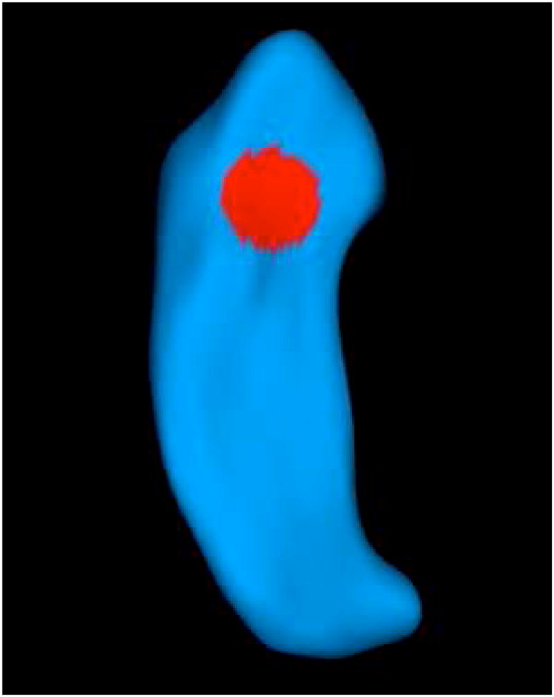
Region-of-interest (ROI) on the surface of a reference hippocampus. The ROI is indicated by the red area.

$${\mathbf{y}}_{ij}(d)={\beta }_0(d)+{\beta }_1(d)t_{ij}+{\beta }_2(d)x_i+{\beta }_3(d)t_{ij}{x}_i+b_i(d)+{\epsilon }_{ij}(d)$$ (3.2)

for i = 1, ···, n, j = 1, ···, m_i, where t_ij is the time taking values in (1, 2, 3, 4, 5), x_i was independently generated from a N(0, 1) distribution, b_i(d) was independently generated from a N(0, 1) distribution, and ε_ij(d) was independently generated from a N(0, 1) distribution. For computational simplicity, we used the generalized estimating equations (2.4), in which s₀ = 1 and $M_i^{(1)}=I_{m_i}$. To assess the Type I and II errors at the voxel level, a region-of-interest (ROI) was selected to include 120 voxels on the reference hippocampus (see Figure 2). We set β(d) = 0₄ for the whole hippocampus and then changed β₃(d) from 0 to various other values for the 120 voxels in the ROI. We applied TETEL and then tested the hypotheses H₀ : β₃(d) = 0 and H₁ : β₃(d) ≠ 0 in the two stages of TETEL across all voxels. The 100 % replications were used to approximate the rejection rate with significance level α = .05. As shown in Table 2, the Type I rejection rates outside of the ROI were relatively accurate for all cases, while the statistical power for rejecting the null hypothesis in the ROI significantly increased with the absolute value of β₃(d).

Table 2.

Comparison of the two stages of TETEL for spatial data: true average rejection rates for voxels inside the ROI and false average rejection rates for voxels outside of the ROI.

β3	Stage	n=40		n=60		n=80
		True	False	True	False	True	False
0.2	Stage 1	0.153	0.071	0.168	0.065	0.205	0.059
	Stage 2	0.247	0.070	0.247	0.065	0.289	0.058
0.4	Stage 1	0.547	0.073	0.558	0.065	0.678	0.059
	Stage 2	0.638	0.072	0.672	0.063	0.756	0.058
0.6	Stage 1	0.659	0.075	0.706	0.066	0.792	0.057
	Stage 2	0.819	0.075	0.812	0.066	0.943	0.056
0.8	Stage 1	0.821	0.073	0.908	0.065	0.992	0.059
	Stage 2	0.907	0.071	0.993	0.065	1.000	0.061

4. Hippocampus shape

4.1. SPHARM representation

For the SPHARM representation, the response is the spatial coordinates at each voxel of the left and right hippocampi; the covariate x_ij = (1, gender_i, age_i, SC_i, race1_i, race2_i, time_ij)^T and β = (β₀, β₁, ···, β₆)^T, where age_i is the age at the baseline, SC is the dummy variable for schizophrenia patients versus healthy controls, and race1 and race2 are, respectively, dummy variables for Caucasian and African American versus other race. Except for time variable, all other covariates are time independent, so we used the estimating equations (2.4), in which s₀ = 3, $M_i^{(1)}=I_{m_i},M_i^{(2)}$, has 1 on the sub-diagonal and 0 elsewhere and $M_i^{(3)}$ has 1 on the two corner components of the diagonal and 0 elsewhere [Qu et al. (2000)]. The Shapiro-Wilk test rejects the normality assumption at many voxels of both the left and right hippocampus structures, therefore our nonparametric AETEL and TAETEL methods are preferred for the analysis of this dataset.

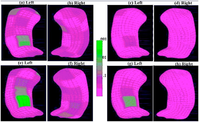
Since our goal is to detect the difference in the SPHARM-PDM surface shape between the schizophrenic and control groups, we used LR_Aetel and LR_{T etel} to carry out the test. The color-coded p-values of the LR_Aetel and LR_{T etel} and their corrected p–values using FDR across the voxels of both the left and right reference hippocampus are shown in Figure 3 [Benjamini and Hochberg (1995), Benjamini and Yekutieli (2001)], in which the top row is for the first stage (LR_Aetel) and the bottom row is for the second stage (LR_{T etel}).

Fig 3.

SPHARM-PDM representation of hippocampal surfaces. The first and third rows are for the first stage (LR_Aetel): the color-coded raw p–value maps of group effect for the left hippocampus (a, b) and the right hippocampus (c, d) and the corresponding color-coded corrected p–value maps of group effect for the left hippocampus (i, j) and the right hippocampus (k, l). The second and fourth rows are for the second stage (LR_{T etel}): the color-coded p–value maps of group effect for the left hippocampus (e, f) and the right hippocampus (g, h) and and the corresponding color-coded corrected p–value maps of group effect for the left hippocampus (m, n) and the right hippocampus (o, p).

The analyses show strong shape differences in the superior, anterior parts of the left hippocampus, at the intersection of CA1 and CA2, previously not shown. Posterior shape changes at the hippocampal tail shown in chronic schizophrenics [Styner et al. (2004)] are detected here already in first episode patients. Furthermore, the results also confirm those reported in Narr et al. (2004) by indicating a strong medial shape difference in the central, left hippocampal body in first episode patients. Comparing the first and second rows, it is clear that TETEL shows advantages in detecting more significant and smoother activation areas.

4.2. M-rep thickness

We first considered the baseline analysis. We used the moment model based on the estimating equations $g({\mathbf{z}}_i,\theta )={\mathbf{x}}_{i1}({\mathbf{y}}_{i1}-{\mathbf{x}}_{i1}^T\beta )$, where y_i1 is the m-rep thickness measured at the baseline for the i-th subject at each medial atom of the left and right hippocampi; x_i1 is an 8 × 1 vector given by x_i1 = (1, gender_i, age_i, SC1_i, SC2_i, race1_i, race2_i, WBV_i1)^T, where SC1 and SC2 were, respectively, dummy variables for haloperidol-treated SC patients and olanzapine-treated SC patients versus healthy controls, and race1 and race2 were, respectively, dummy variables for Caucasian and African American versus other race; β = (β₀, β₁, ···, β₇)^T. Existing statistical methods of the image data in SPM require that the error distribution be Gaussian and the variance be constant. The Shapiro-Wilk normality test was applied to check this parametric assumption of the general linear model at each atom for the left hippocampus and right hippocampus using the residuals. Figures 4(c) and (e) show that the Shapiro-Wilk test rejects the normality assumption at many atoms of both the left and right hippocampus structures, therefore our nonparametric AETEL method is prefered for the analysis of this dataset. Because the m-rep thickness measures at 24 atoms do not have strong spatial pattern, we do not use TETEL for the analysis of the m-rep thickness.

Since our goal is to detect the difference in the thickness of the hippocampus across the three groups, we set up the null hypotheses H₀ : β₄ = β₅ = 0 at all 24 atoms for both the left and right hippocampi. Accordingly, we have

$$R=\left(\begin{array}{cccccccc}0& 0& 0& 1& 0& 0& 0& 0\\ 0& 0& 0& 0& 1& 0& 0& 0\end{array}\right),$$

and b₀ = (0, 0)^T. We used LR_Aetel to carry out the test. The color-coded p-values of the LR_Aetel across the atoms of both the left and right reference hippocampus are shown in Figures 6(a) and (b). The false discovery rate approach was used to correct for multiple comparisons, and the resulting adjusted p-values were shown in Figures 6(c) and (d). Before correcting for multiple comparisons, there was a significant group difference in m-rep thickness at the upper central atoms in the left hippocampus and some area in the right hippocampus. However, there is no significant group effect at any atoms after correcting for multiple comparisons.

Fig 6.

M-rep representation of hippocampal structures: The top row is for the baseline analysis: the color-coded uncorrected p–value maps of group effect for (a) the left hippocampus and (b) the right hippocampus; the color-coded corrected p–value maps of group effect for (c) the left hippocampus and (d) the right hippocampus after correcting for multiple comparisons. The bottom row is for the longitudinal analysis: the color-coded uncorrected p–value maps of group effect for (e) the left hippocampus and (f) the right hippocampus; the color-coded corrected p–value maps of group effect for (g) the left hippocampus and (h) the right hippocampus after correcting for multiple comparisons.

Secondly, we did a longitudinal data analysis. The advantage of a longitudinal study over a baseline study is that it allows us to determine (i) whether the change patterns of the response are similar or not across the three groups; (ii) whether, on average over time, there is a difference in the response across the three groups. We chose

$${\mathbf{x}}_{ij}={(1,{\text{gender}}_i,{\text{age}}_i,\text{SC}{1}_i,\text{SC}{2}_i,\mathit{race}{1}_i,\mathit{race}{2}_i,{\mathit{WBV}}_{ij},{\mathit{time}}_{ij},\text{SC}{1}_i\ast {\mathit{time}}_{ij},\text{SC}{2}_i\ast {\mathit{time}}_{ij})}^T$$

and β = (β₀, β₁, ···, β₁₀)^T, where WBV is a time-dependent covariate.

Since WBV is a time-dependent covariate, we needed to verify its appropriate type. Moreover, from a neuroscience point of view, the m-rep thickness at each atom serves as a local volumetric measure and covaries with WBV. We started with type III and used the GEE estimating equations in (2.2) with V_i = I_mi. Then we used the type II equations specified in (2.5) and tested whether WBV is type II against type III. The LR_Aetel did not reject for almost all 24 atoms, suggesting WBV is a type II covariate for most atoms. Furthermore, we used the type I equations specified in (2.3) and tested whether WBV is type I against type II. The LR_Aetel rejected that WBV was of type I for most atoms (Figure 5). This indicates the invalidity of some type I equations. We used the goodness-of-fit statistic in Zhu et al. (2008) to test whether some of the extra equations added for type I, such as

Fig 5.

M-rep representation of hippocampal structures: maps of −log₁₀(p)-values for testing WBV as a type I time-dependent covariate (black) and a type II time-dependent covariate (red): (a) uncorrected −log₁₀(p)-values for left hippocampus; (b) uncorrected −log₁₀(p)-values for right hippocampus; (c) corrected −log₁₀(p)-values for left hippocampus; (d) corrected −log₁₀(p)-values for right hippocampus; (e) the goodness-of-fit test for the equation E{∂_βμ_i2(β)[y_i3 − μ_i3(β)]} = 0 for the 3-rd atom on the left hippocampus; (f) the goodness-of-fit test for the equation E{∂_βμ_i2(β)[y_i3 − μ_i3(β)]} = 0 for the 14-th atom on the right hippocampus.

$$E\{{\partial }_{{\beta }_l}{\mu }_{is}(\beta )[{\mathbf{y}}_{ij}-{\mu }_{ij}(\beta )]\}=0\text{for}\text{all}s<j,j=1,\cdots ,m_i,$$

were not valid. For instance, for the 3rd atom on the left hippocampus, the p–value for the goodness-of-fit test for the newly added equation E{∂_βlμ_i2(β)[y_i3 − μ_i3(β)]} = 0 was smaller than 0.001 (Figure 5(e)); for the 14-th atom on the right hippocampus, the p–value for the goodness-of-fit test for the newly added equation E{∂_βlμ_i2(β)[y_i3 − μ_i3(β)]} = 0 was smaller than 0.001 (Figure 5(f)). Therefore, we treated WBV as a type II time-dependent covariate and used the corresponding estimating equation for the longitudinal data analysis.

To determine whether the change patterns of the thickness of the hippocampus over time are similar or not across the three groups, we tested the null hypotheses H₀ : β₉ = β₁₀ = 0 (β₉ and β₁₀ are the coefficients of the interaction terms of group and time) at all 24 atoms for each of the left hippocampus and the right hippocampus. It turned out that the interaction terms were not significant for most atoms. Next we deleted the interaction terms and tried to look at whether there are differences in the responses across the three groups on average over time with respect to the null hypotheses H₀ : β₃ = β₄ = 0 at all 24 atoms for each of the left hippocampus and the right hippocampus. Again we only found that there was a significant difference through time in m-rep thickness at the upper central atoms in the left hippocampus across schizophrenia patients and healthy controls groups after correcting for multiple comparisons, but the differences were not significant at other atoms, nor at any atoms on the right hippocampus. The color-coded p-values of the LR_Aetel across the atoms of both the left and right reference hippocampus are shown in Figures 6(e) and (f), and the corrected p-values were shown in Figures 6(g) and (h). Before correcting for multiple comparisons, there was a significant group difference in m-rep thickness at the upper central atoms in the left hippocampus, and the significance level is larger than that of the baseline analysis. After correcting for multiple comparisons, there is still a significant group effect at the upper central atoms in the left hippocampus [Benjamini and Hochberg (1995), Benjamini and Yekutieli (2001)].

We compared the results by making the assumption that WBV was a type II time-dependent and also a type III time-dependent covariate. Treating WBV as a type II time-dependent covariate lowered the p–values, making some non-significant p–values for the group effect significant. On the other hand, we found that all the standard deviations associated with the parameter estimates treating WBV as a type II time-dependent covariate were uniformly less than those treating WBV as a type III, which confirms that treating WBV as a type II gains efficiency by making use of more correct estimating equations. Table 3 compares the standard deviations of the parameter estimates between treating WBV as a type II time-dependent covariate and a type III time-dependent covariate at atom 11 of the left hippocampus.

Table 3.

Standard deviation comparison of the parameter estimates between treating WBV as a type II time-dependent covariate and a type III time-dependent covariate at atom 11 of the left hippocampus.

	intercept	gender	age	SC1	SC2	race1	race2	WBV	time
type III	0.367	0.078	0.007	0.062	0.058	0.097	0.102	0.237	0.022
type II	0.344	0.075	0.005	0.058	0.054	0.094	0.100	0.221	0.018

The longitudinal analysis increased the significance level at those significant atoms for the group effect, compared to the baseline analysis. We were also able to observe the change difference across groups through time, although it is not much. Both the baseline analysis and longitudinal analysis suggest that there is an asymmetric aspect in that the left hippocampus shows larger regions of significance than the right one, and the significant positions of the group differences are around the lateral dentate gyrus and medial CA4 body regions for the left hippocampus.

5. Discussion

We have developed TAETEL for spatial analysis of neuroimaging data from longitudinal studies. We have shown that AETEL allows us to efficiently analyze longitudinal data with different time-dependent covariate types. We have specifically combined all the data in the neighborhood of each voxel (or pixel) on a 3D volume (or 2D surface) with appropriate weights to calculate adaptive parameter estimates and adaptive test statistics. We have used simulation studies to examine the finite sample performance of AETEL and TAETEL. In our longitudinal schizophrenia study, we have used the boundary and medial shape of the hippocampus to detect differences in morphological changes of the hippocampus across time between schizophrenic patients and healthy subjects. For the m-rep thickness, we have found that WBV is an important time-dependent covariate. Potential applications of our methodology include understanding normal and abnormal brain development, and identifying the neural bases of the pathophysiology and etiology of neurodegenerative and neuropsychiatric disorders.

Many issues still merit further research. One major issue is to develop a test procedure, such as random field theory and resampling methods, to correct for multiple comparisons in order to control the family-wise error rate under the moment model (2.1). Another major issue is to extend the test procedure to conduct cluster size inference and examine its performance in controlling the Type I error rate. The test procedure may lead to a simple cluster size test (cluster size test assesses significance for all sizes of the connected regions greater than a given primary threshold). It is also interesting to consider models with nonparametric components using TETEL.

APPENDIX A: ASSUMPTIONS AND PROOFS

The following assumptions are needed to facilitate the technical details, although they are not the weakest possible conditions.

Assumption A: {z_i(d): d ∈ } forms an independent and identical sequence.

Assumption B: For each d ∈ , the true value θ₀(d) of θ(d) is the unique solution to E{g(z(d), θ (d))} = 0 and θ₀(d) is an interior point of the compact set Θ ⊂ R^p.

Assumption C: In a neighborhood of the true value θ₀(d), g(z(d), θ(d)) has a second-order continuous derivative with respect to θ(d) and ||∂_θ(d)g(z(d), θ(d))||, || $\left|\right|{\partial }_{\theta (d)}^2\mathbf{g}(\mathbf{z}(d),\theta (d))\left|\right|$, and ||g(z(d), θ(d))||³ are bounded by some integrable function G(z(d)) with E_F {sup_δ∈ G(z(d))} < ∞.

Assumption D: The rank of E{∂θ_(d)g(z(d), θ₀(d))} is p and

$$\underset{d\in \mathcal{D}}{min}{\lambda }_{min}E\{\mathbf{g}(\mathbf{z}(d),{\theta }_0(d)){\mathbf{g}}^T(\mathbf{z}(d),{\theta }_0(d))\}>0,$$

where λ_min(·) denotes the smallest eigenvalue of a matrix.

Assumption E: F_η(u)dη is absolutely continuous with respect to Lebesgue measure on Π, where F_η(u) is the true cumulative distribution function of η^T x.

Assumption F: ||a(x)||³ is bounded by some integrable function G₁(x).

Assumption G: For each d ∈ , θ₀(d) is the unique maxima of the function L_Aetal(θ, d) = − log(E[exp(t^*(θ)^T {g(z_i(d), θ)−E[g(z_i(d), θ)]})]), where t^*(θ) is the solution of E[exp(t^*T g(z_i(d), θ)] = 0.

Assumption H: For each d ∈ , E[sup_θ∈Θ sup_{t∈ (θ)} exp(t^T g(z_i(d), θ)] < ∞, where ( θ) is a compact set including t^*T (θ) as an interior point.

Assumption I: For each d ∈ , rank[E{Σ_{d′∈N0(d)⊂{d}} ∂θg(z(d′), θ₀(d))}] =p and

$$\underset{d\in \mathcal{D}}{min}{\lambda }_{min}E\{{[\sum _{d^{\prime }\in N_0(d)\cup \{d\}}\mathbf{g}(\mathbf{z}(d^{\prime }),{\theta }_0(d))]}^{\otimes 2}\}>0,$$

where λ_min(·) denotes the smallest eigenvalue of a matrix and N₀(d) = {d′ ∈ N(d): θ₀(d′) = θ₀(d)}.

Lemma A1

If Assumptions A, C, and D are satisfied, then for any 1/3 < δ < 1/2 and (δ) = {t : ||t|| ≤ n^−δ}, sup_{θ∈Θ,t∈ (δ),1≤i≤n} |t^T g(z_i, θ)| → 0 and (δ) ⊂ (a₁; θ) = {t : t^T g(z_i, θ) ∈ [−a₁, a₁]} for all θ ∈ Θ, where a₁ > 0.

Proof of Lemma A1

It follows from Assumptions A and C that max_1≤i≤n sup_θ∈Θ |g(z_i, θ)| = O(n^1/3). Then, we have

$$\underset{1\le i\le n}{max}\underset{\mathbf{t}\in {\mathcal{T}}_n(\delta );\theta \in \mathrm{\Theta }}{sup}\mid {\mathbf{t}}^T\mathbf{g}({\mathbf{z}}_i,\theta )\mid \le O(n^{1/3})n^{-\delta }=O(n^{1/3-\delta })\to 0$$

almost surely. Thus, Lemma A1 follows.

Lemma A2

If Assumptions A–E are satisfied and θ̄ = θ₀ + n^−δ₀u, then t̄( θ̄) = argmax_{t∈ (a1; θ̄)} F_n(θ̄, t) exists and t̄( θ̄) = O(n^−δ₀), where ||u|| = 1 and $F_n(\theta ,\mathbf{t})=-n^{-1}{\sum }_{i=1}^{n}exp({\mathbf{t}}^T\mathbf{g}({\mathbf{z}}_i,\theta ))$.

Proof of Lemma A2

It can be seen that F_n(θ, t) is an analytical function of t. Thus, t̃ = argmax_{t∈ (η)} F_n(θ̄, t) exists. Using a Taylor’s series expansion, we can show that

$$\begin{array}{l}-1=F_n(\overline{\theta },\mathbf{0})\le F_n(\overline{\theta },\stackrel{\sim }{\mathbf{t}})\\ =-1-{\stackrel{\sim }{\mathbf{t}}}^T\sum _{i=1}^n{\mathbf{g}}_i(\overline{\theta })/n-0.5{\stackrel{\sim }{\mathbf{t}}}^T\sum _{i=1}^{n}exp({\stackrel{.}{\mathbf{t}}}^T{\mathbf{g}}_i(\overline{\theta })){\mathbf{g}}_i{(\overline{\theta })}^{\otimes 2}\stackrel{\sim }{\mathbf{t}}/n,\end{array}$$ (A.1)

where g_i(θ) = g(z_i, θ), a^⊗2 = aa^T, and t˙ is on the line joining t̃ and 0. Moreover, because

$$n^{-1}\sum _{i=1}^{n}exp({\stackrel{.}{\mathbf{t}}}^T{\mathbf{g}}_i(\overline{\theta })){\mathbf{g}}_i{(\overline{\theta })}^{\otimes 2}\to E\{\mathbf{g}{(\mathbf{z},{\theta }_0)}^{\otimes 2}\},$$ (A.2)

it follows from (A.1) that $\left|\right|\stackrel{\sim }{\mathbf{t}}\left|\right|\le \left|\right|n^{-1}{\sum }_{i=1}^n\mathbf{g}({\mathbf{z}}_i,\overline{\theta })\left|\right|=O(n^{-{\delta }_0})=o(n^{-\delta })$ for all δ₀ > δ. Therefore, for large n, t̃ ∈ int( (δ)) ⊂ (a₁; θ̄) and ∂_tF_n(θ̄, t̃) = 0. Because of the concavity of F_n(θ̄, t) in t, we have t̄(θ̄) = t̃ and F_n(θ̄, t̃) = F_n(θ̄, t̃) max_{t∈ (a1;θ̄)}. Moreover, we have

$${\partial }_t{F}_n(\overline{\theta },\overline{\mathbf{t}}(\overline{\theta }))={\partial }_t{F}_n(\overline{\theta },\mathbf{0})+{\partial }_t^2{F}_n(\overline{\theta },\stackrel{.}{\mathbf{t}})\overline{\mathbf{t}}(\overline{\theta }).$$

Because max_1≤i≤n |t˙^T g_i(θ)| = o(1), we have

$$\overline{\mathbf{t}}(\overline{\theta })=-{[\sum _{i=1}^n{\mathbf{g}}_i{(\overline{\theta })}^{\otimes 2}]}^{-1}\sum _{i=1}^n{\mathbf{g}}_i(\overline{\theta })+o(n^{-{\delta }_0}).$$

Proof of Theorem 2.1

For notational simplicity, we define θ̂ = θ̂_Aetel, t̂ = t̂_Aetel, and h_i(θ) = g(z_i, θ) for i = 1, ···, n and h_n+1(θ) = g_n+1(θ). We also define

$$\begin{array}{l}{G}_n(\theta ,\mathbf{t})=-log({(n+1)}^{-1}\sum _{i=1}^{n+1}exp({\mathbf{t}}^T(g_i(\theta )-\overline{g}(\theta )))),\\ S_n(\theta )=\left(\begin{array}{cc}{S}_{n,11}& S_{n,12}\\ S_{n,21}& S_{n,22}\end{array}\right)={(n+1)}^{-1}\left(\begin{array}{cc}{\sum }_{i=1}^{n+1}{\mathbf{h}}_i(\theta ){\mathbf{h}}_i^T(\theta )& -{\sum }_{i=1}^{n+1}{({\partial }_{\theta }{\mathbf{h}}_i(\theta ))}^T\\ -{\sum }_{i=1}^{n+1}{\partial }_{\theta }{\mathbf{h}}_i(\theta )& \mathbf{0}\end{array}\right),\\ S=S(t_0,{\theta }_0)=\left(\begin{array}{cc}{S}_{11}& S_{12}\\ S_{21}& S_{22}\end{array}\right)=\left(\begin{array}{cc}E[{\mathbf{g}}^{\otimes 2}({\mathbf{z}}_i,{\theta }_0)]& -E{[{\partial }_{\theta }\mathbf{g}({\mathbf{z}}_i,{\theta }_0)]}^T\\ -E[{\partial }_{\theta }\mathbf{g}({\mathbf{z}}_i,{\theta }_0)]& \mathbf{0}\end{array}\right),\end{array}$$

where $\overline{\mathbf{g}}(\theta )={\sum }_{i=1}^{n+1}{\mathbf{g}}_i(\theta )/(n+1)$.

The proof of Theorem 2.1 (a) consists of two steps as follows.

• Step 1G_n(θ, t̄( θ)) attains its minimum value at some point θ̃ in the interior of the ball ||θ − θ₀|| ≤ n^−δ₀.
• Step 2 $\sqrt{n}({\widehat{\theta }}_{\mathit{Aetel}}-{\theta }_0)$ converges to ν₀ as described in Theorem 1 (a).

In Step 1, we can use Assumptions (A)–(D) to show that sup_θ∈Θ |h_n+1(θ)+ a_nE[g(z, θ)]| = O_p(a_nn^−1/2) (van der Vaart and Wellner, 1996). Thus, the contribution from h_n+1(θ) is negligible. Then, we can follow the proof of Lemma 1 in Qin and Lawless (1996) to prove that G_n(θ̄, t̄(θ̄)) = O(n^−2δ₀) and G_n(θ₀, t̄( θ₀)) = O(n⁻¹ log log n) = o(n^−2δ₀). Since G_n(θ, t̄( θ)) is a continuous function about θ as ||θ − θ₀|| ≤ n^−2δ₀, G_n(θ, t̄(θ)) has a minimum value in the interior of this ball.

In Step 2, for the adjusted ETEL, we have

$${\ell }_{\mathit{Aetel}}(\mathbf{t},\theta )={(n+1)}^{-1}\sum _{i=1}^{n+1}log[\frac{(n+1)exp({\mathbf{t}}^T{\mathbf{h}}_i(\theta ))}{{\displaystyle \sum _{j=1}^{n+1}}exp({\mathbf{t}}^T{\mathbf{h}}_j(\theta ))}].$$

Similar to Theorem 2 of Schennach (2007), we can obtain the first order conditions for θ̂ and t̂ as follows:

$$\begin{array}{l}{Q}_{1,n}(\mathbf{t},\theta )={(n+1)}^{-1}\sum _{i=1}^{n+1}{\mathbf{h}}_i(\theta )exp({\mathbf{t}}^T{\mathbf{h}}_i(\theta ))=0,\\ Q_{2,n}(\mathbf{t},\theta )={(n+1)}^{-1}\sum _{i=1}^{n+1}\{1-\frac{(n+1)exp({\mathbf{t}}^T{\mathbf{h}}_i(\theta ))}{{\displaystyle \sum _{j=1}^{n+1}}exp({\mathbf{t}}^T{\mathbf{h}}_j(\theta ))}\}=0.\end{array}$$

Expanding the above first order conditions for θ̄ and t̄ around θ₀ and t₀ = 0 leads to

$$\begin{array}{l}0=Q_{1,n}(0,{\theta }_0)+[{\{{\partial }_{\theta }{Q}_{1,n}(0,{\theta }_0)\}}^T(\widehat{\theta }-{\theta }_0)+{\partial }_t{Q}_{1,n}(0,{\theta }_0)(\widehat{\mathbf{t}}-0)]\{1+o_p(1)\},\\ 0=Q_{2,n}(0,{\theta }_0)+[{\partial }_{\theta }{Q}_{2,n}(0,{\theta }_0)(\widehat{\theta }-{\theta }_0)+{\{{\partial }_t{Q}_{2,n}(0,{\theta }_0)\}}^T(\widehat{\mathbf{t}}-0)]\{1+o_p(1)\}.\end{array}$$

Therefore, it can be shown that

$$\left(\begin{array}{c}\widehat{\mathbf{t}}\\ \widehat{\theta }-{\theta }_0\end{array}\right)=S_n^{-1}({\theta }_0)\left(\begin{array}{c}{Q}_{1,n}(0,{\theta }_0)\\ 0\end{array}\right)\{1+o_p(1)\},$$

where

$$S_n({\theta }_0)={\left(\begin{array}{cc}{\partial }_t{Q}_{1,n}& {({\partial }_{\theta }{Q}_{1,n})}^T\\ {({\partial }_t{Q}_{2,n})}^T& {\partial }_{\theta }{Q}_{2,n}\end{array}\right)}_{(0,{\theta }_0)}=\frac{1}{n+1}\left(\begin{array}{cc}\sum {\mathbf{h}}_i({\theta }_0){\mathbf{h}}_i^T({\theta }_0)& -\sum {({\partial }_{\theta }{\mathbf{h}}_i({\theta }_0))}^T\\ -\sum {\partial }_{\theta }{\mathbf{h}}_i({\theta }_0)& 0\end{array}\right).$$

The law of large number ensures that S_n(θ₀) → S. Thus, with some simple calculations, we can prove that

$$\sqrt{n}(\widehat{\theta }-{\theta }_0)=\sqrt{n}{S}_{22.1}^{-1}{S}_{21}{S}_{11}^{-1}\frac{1}{n+1}\sum _{i=1}^n\mathbf{g}({\mathbf{z}}_i,{\theta }_0)+o_p(1),$$ (A.3)

where $S_{22.1}=-S_{21}{S}_{11}^{-1}{S}_{12}$. Applying the central limit theorem completes the proof of Theorem 1 (a).

Following the proof of Theorem 2 in Qin and Lawless (1994), we can obtain the proof of Theorem 2.1 (b) and (c).

Lemma A3

If Assumptions A, B, G, and H are true, then we have the following results:

1. t̄(θ, d) → t^*(θ, d) uniformly for θ ∈ Θ;

2. ℓ_Aetel(θ, d) → L_Aetel(θ, d) uniformly for θ ∈ Θ, where $\widehat{\mathbf{t}}(\theta ,d)={\mathit{argmax}}_t\{-{\sum }_{i=1}^{n}exp({\mathbf{t}}^T\mathbf{g}({\mathbf{z}}_i(d),\theta ))-exp({\mathbf{t}}^T{\mathbf{g}}_{n+1}(\theta ,d))\}$, in which ${\mathbf{g}}_{n+1}(\theta ,d)=-a_n{n}^{-1}{\sum }_{i=1}^n\mathbf{g}({\mathbf{z}}_i(d),\theta )$.

Proof of Lemma A3

We prove (i) as follows. First, it follows from the assumptions that $\widehat{M}(\mathbf{t};\theta ,d)=n^{-1}{\sum }_{i=1}^{n}exp({\text{t}}^T\mathbf{g}({\mathbf{z}}_i(d),\theta ))+n^{-1}exp({\mathbf{t}}^T{\mathbf{g}}_{n+1}(\theta ,d)){\to }^{p}E[exp({\mathbf{t}}^T\mathbf{g}(\mathbf{z}(d),\theta ))]$ uniformly over the compact set {(t, θ) : t ∈ (θ), θ ∈ Θ}. Second, following the arguments in Step 1 of Theorem 10 in Schennach (2007), we can complete the proof of (i).

We prove (ii) as follows. First, with some algebraic calculations, we get ${\ell }_{\mathit{Aetel}}(\theta ,d)=-log({(n+1)}^{-1}\widehat{\mathbf{t}}{(\theta ,d)}^T[{\sum }_{i=1}^n\mathbf{g}({\mathbf{z}}_i(d),\theta )+{\mathbf{g}}_{n+1}(\theta ,d)])+{(n+1)}^{-1}\widehat{\mathbf{t}}{(\theta ,d)}^T[{\sum }_{i=1}^n\mathbf{g}({\mathbf{z}}_i(d),\theta )+{\mathbf{g}}_{n+1}(\theta ,d)]$. Second, it follows from the assumptions and (i) that (ii) is true.

Lemma A4

If Assumptions A, B, G, and H are true, then we have

$$\omega (d^{\prime };d)=[1+o_p(1)]\mathbf{1}({\mathrm{\Delta }}_{\ast }(d,d^{\prime })\ne \mathbf{0})+exp(-2n{A}_{\ast }(d,d^{\prime })[1+o_p(1)]/C_n)\mathbf{1}({\mathrm{\Delta }}_{\ast }(d,d^{\prime })\ne \mathbf{0}),$$ (A.4)

where Δ_*(d, d′) = θ₀(d) − θ₀(d′) and A_*(d, d′) = L_Aetel(θ₀(d), d) − L_Aetel(θ₀(d′), d).

Proof of Lemma A4

We consider voxel d′ ∈ N(d) with θ₀(d′) ≠ θ₀(d). It can be shown that LR_Aetel(d′; d) can be decomposed into three terms. The first term is −2(n + 1){ℓ_Aetel(θ̄(d′); d) − ℓ_Aetel(θ₀(d′); d)}, which is o_p((n + 1)). The second term is −2(n + 1){ℓ_Aetel(θ₀(d′); d) − ℓ_Aetel(θ₀(d); d)}, which is asymptotically equivalent to −2(n + 1)A_*(d, d′)[1 + o_p(1)] based on Lemma A3. The third term is −2(n + 1){ℓ_Aetel(θ₀(d); d) − ℓ_Aetel(θ̄(d); d)}, which is asymptotically χ² distributed, that is O_p(1). Thus, we obtain ω(d′; d) = exp(−2(n + 1)A_*(d, d′)[1 + o_p(1)]).

We consider voxel d′ ∈ N(d) with θ₀(d′) = θ₀(d). It can be shown that LR_Aetel(d′; d) can be decomposed into two terms. The first term is −2(n+1){ℓ_Aetel(θ̄(d′); d) − ℓ_Aetel(θ₀(d); d)}, which is O_p(1). The second term is −2(n + 1){ℓ_Aetel(θ₀(d); d) − ℓ_Aetel(θ̄(d); d)}, which is also O_p(1). Thus, we obtain $\omega (d^{\prime };d)=exp(-O_p(1)C_n^{-1})=o_p(1)$.

Lemma A5

If Assumptions A–C, G and H are satisfied and θ̄ = θ₀(d) + n^−δ₀u, then t̄(θ̄(d); d) = argmax_{t∈ (a1;θ̄)} F_n(θ̄, t; d) exists and t̄(θ̄; d) = O (n^−δ₀), where ||u|| = 1 and $F_n(\theta ,\mathbf{t};d)=-{(n+1)}^{-1}{\sum }_{i=1}^{n}exp({\mathbf{t}}^T\stackrel{\sim }{\mathbf{g}}({\mathbf{z}}_i(d),\theta ;d))-{(n+1)}^{-1}exp({\mathbf{t}}^T{\stackrel{\sim }{\mathbf{g}}}_{n+1}(\theta ,d))$, in which ${\stackrel{\sim }{\mathbf{g}}}_{n+1}(\theta ,d)=-a_n{n}^{-1}{\sum }_{i=1}^n\stackrel{\sim }{\mathbf{g}}({\mathbf{z}}_i(d),\theta ;d)$.

Proof of Lemma A5

The proof of Lemma A5 is similar to that of Lemma A2. We only highlight the three key differences as follows. First, we note that

$$\underset{1\le i\le n}{max}\underset{\theta \in \mathrm{\Theta }}{sup}\mid \stackrel{\sim }{\mathbf{g}}({\mathbf{z}}_i(d),\theta ;d))\mid \le \sum _{d^{\prime }\in N(d)\cup \{d\}}\omega (d^{\prime };d)\underset{1\le i\le n}{max}\underset{\theta \in \mathrm{\Theta }}{sup}\mid \mathbf{g}({\mathbf{z}}_i(d^{\prime }),\theta ))\mid =O(n^{1/3}).$$

Second, similar to equation (A.2), it follows from Lemma A4 that

$${(n+1)}^{-1}\sum _{i=1}^{n}exp({\stackrel{.}{\mathbf{t}}}^T\stackrel{\sim }{\mathbf{g}}({\mathbf{z}}_i(d),\theta ;d))\stackrel{\sim }{\mathbf{g}}{({\mathbf{z}}_i(d),\theta ;d)}^{\otimes 2}\to E\{{[\sum _{d^{\prime }\in N_0(d)\cup \{d\}}\mathbf{1}({\mathrm{\Delta }}_{\ast }(d,d^{\prime })=\mathbf{0})\mathbf{g}(\mathbf{z}(d^{\prime }),{\theta }_0(d))]}^{\otimes 2}\},$$

which is positive definite based on assumption I. Third, we have

$$\begin{array}{l}\left|\right|\stackrel{\sim }{\mathbf{t}}(d)\left|\right|\le \left|\right|{(n+1)}^{-1}\sum _{i=1}^{n+1}\stackrel{\sim }{\mathbf{g}}({\mathbf{z}}_i(d),\theta ;d)\left|\right|\le \sum _{d^{\prime }\in N(d)\cup \{d\}}{(n+1)}^{-1}\omega (d^{\prime };d)\left|\right|\sum _{i=1}^n\mathbf{g}({\mathbf{z}}_i(d^{\prime }),\overline{\theta })\left|\right|\\ =\sum _{d\text{'}\in N(d)\cup \{d\}}{O}_p(n^{-{\delta }_0})[\mathbf{1}({\mathrm{\Delta }}_{\ast }(d,d^{\prime })=\mathbf{0})+O_p(exp(-2n{A}_{\ast }(d,d^{\prime })/C_n))\mathbf{1}({\mathrm{\Delta }}_{\ast }(d,d^{\prime })\ne \mathbf{0})],\end{array}$$

which is O_p(n^−δ₀).

Proof of Theorem 2.2

We can combine the results in Lemmas A3–A5 and the arguments in the proof of Theorem 1 to finish the proof of Theorem 2.2.

References

- 1.Almli CR, Rivkin MJ, McKinstry RC Brain Development Cooperative Group. The NIH MRI study of normal brain development (objective-2): newborns, infants, toddlers, and preschoolers. NeuroImage. 2007;35:308–325. doi: 10.1016/j.neuroimage.2006.08.058. [DOI] [PubMed] [Google Scholar]
- 2.Arndt S, Cohen G, Alliger RJ, Swayze VW, Andreasen NC. Problems with ratio and proportion measures of imaged cerebral structures. Psychiatry Res. 1991;40:7989. doi: 10.1016/0925-4927(91)90031-k. [DOI] [PubMed] [Google Scholar]
- 3.Ashburner J, Friston KJ. Voxel-based morphometry: the methods. NeuroImage. 2000;11:805–821. doi: 10.1006/nimg.2000.0582. [DOI] [PubMed] [Google Scholar]
- 4.Beckmann CF, Jenkinson M, Smith SM. General multilevel linear modeling for group analysis in fMRI. NeuroImage. 2003;20:1052–1063. doi: 10.1016/S1053-8119(03)00435-X. [DOI] [PubMed] [Google Scholar]
- 5.Benjamini Y, Hochberg Y. Controlling the false discovery rate: a practical and powerful approach to multiple testing. Journal of the Royal Statistical Society, Ser B. 1995;57:289–300. [Google Scholar]
- 6.Benjamini Y, Yekutieli D. The control of the false discovery rate in multiple testing under dependency. The Annals of Statistics. 2001;29:1165–1188. [Google Scholar]
- 7.Bowman FD, Caffo B, Bassett SS, Kilts C. A Bayesian hierarchical framework for spatial modeling of fMRI data. Neuroimage. 2008;39:146–156. doi: 10.1016/j.neuroimage.2007.08.012. [DOI] [PMC free article] [PubMed] [Google Scholar]
- 8.Cao J, Worsley KJ. Applications of random fields in human brain mapping. In: Moore M, editor. Spatial Statistics: Methodological Aspects and Applications. New York: Springer; 2001. p. 159. [Google Scholar]
- 9.Chen JH, Variyath AM, Abraham B. Adjusted empirical likelihood and its properties. Journal of Computational and Graphical Statistics. 2008;17:426–443. [Google Scholar]
- 10.Chung MK, Dalton KM, Davidson RJ. Tensor-based cortical surface morphometry via weighted spherical harmonic representation. IEEE Transactions on Medical Imaging. 2007;26:566–581. doi: 10.1109/TMI.2008.918338. [DOI] [PubMed] [Google Scholar]
- 11.Diggle P, Heagerty P, Liang KY, Zeger S. Analysis of Longitudinal Data. 2. Oxford University Press; New York: 2002. [Google Scholar]
- 12.Dryden I, Mardia K. Statistical Shape Analysis. New York: John Wiley and Sons; 1998. [Google Scholar]
- 13.Duvernoy H. The Human Hippocampus. New York, NY: Springer Verlag; 2005. [Google Scholar]
- 14.Friston KJ. Statistical Parametric Mapping: the Analysis of Functional Brain Images. Academic Press; London: 2007. [Google Scholar]
- 15.Friston KJ, Holmes AP, Poline JB, Price CJ, Frith CD. Detecting activations in PET and fMRI: levels of inference and power. NeuroImage. 1996;4:223–235. doi: 10.1006/nimg.1996.0074. [DOI] [PubMed] [Google Scholar]
- 16.Friston KJ, Stephan KE, Lund TE, Morcom A, Kiebel S. Mixed-effects and fMRI studies. NeuroImage. 2005;24:244–252. doi: 10.1016/j.neuroimage.2004.08.055. [DOI] [PubMed] [Google Scholar]
- 17.Golland P, Grimson W, Kikinis R. Statistical shape analysis using fixed topology skeletons: corpus callosum study. Information Processing in Medical Imaging. 1999:382–388. [Google Scholar]
- 18.Hansen L. Large sample properties of generalized method of moments estimators. Econometrica. 1982;50:1029–1054. [Google Scholar]
- 19.Hayasaka S, Phan LK, Liberzon I, Worsley KJ, Nichols TE. Nonstationary cluster-size inference with random field and permutation methods. NeuroImage. 2004;22:676–687. doi: 10.1016/j.neuroimage.2004.01.041. [DOI] [PubMed] [Google Scholar]
- 20.Hecke WV, Sijbers J, Backer SD, Poot D, Parizel PM, Leemans A. On the construction of a ground truth framework for evaluating voxel-based diffusion tensor MRI analysis methods. NeuroImage. 2009;46:692–707. doi: 10.1016/j.neuroimage.2009.02.032. [DOI] [PubMed] [Google Scholar]
- 21.Huettel SA, Song AW, McCarthy G. Functional Magnetic Resonance Imaging. Sinauer Associates, Inc; 2004. [Google Scholar]
- 22.Jones DK, Symms DK, Cercignani M, Howard RJ. The effect of filter size on VBM analyses of DT-MRI data. NeuroImage. 2005;26:546–554. doi: 10.1016/j.neuroimage.2005.02.013. [DOI] [PubMed] [Google Scholar]
- 23.Lai TL, Small D. Marginal regression analysis of longitudinal data with time-dependent covariates: a generalized method-of-moments approach. Journal of the Royal Statistical Society , Ser B. 2007;69:79–99. [Google Scholar]
- 24.Lau JC, Lerch JP, Sled JG, Henkelman RM, Evans AC, Bedell BJ. Longitudinal neuroanatomical changes determined by deformation-based morphometry in a mouse model of alzheimer’s disease. NeuroImage. 2008;42:19–27. doi: 10.1016/j.neuroimage.2008.04.252. [DOI] [PubMed] [Google Scholar]
- 25.Liang KY, Zeger SL. Longitudinal data analysis using generalized linear models. Biometrika. 1986;73:13–22. [Google Scholar]
- 26.Lieberman JA, Tollefson GD, Charles C, Zipursky R, Sharma T, Kahn RS, Keefe RSE, Green AI, Gur RE, McEvoy J, Perkins D, Hamer RM, Gu H, Tohen M. Antipsychotic drug effects on brain morphology in first-episode psychosis. Archives of General Psychiatry. 2005;62:361–70. doi: 10.1001/archpsyc.62.4.361. [DOI] [PubMed] [Google Scholar]
- 27.Lindquist M, Wager T. Spatial smoothing in fmri using prolate spheroidal wave functions. Human Brain mapping. 2008;29:12761287. doi: 10.1002/hbm.20475. [DOI] [PMC free article] [PubMed] [Google Scholar]
- 28.Liu Y, Chen JH. Adjusted empirical likelihood with high-order precision. Annals of Statistics. 2010 in press. [Google Scholar]
- 29.Logan BR, Rowe DB. An evalution of thresholding techniques in fMRI analysis. NeuroImage. 2004;22:95–108. doi: 10.1016/j.neuroimage.2003.12.047. [DOI] [PubMed] [Google Scholar]
- 30.Luo H, Puthusserypady S. A sparse Bayesian method for determination of flexible design matrix for fMRI data analysis. IEEE Transactions on Circuits and Systems I-Regular Papers. 2005;52:2699–2706. [Google Scholar]
- 31.Luo W, Nichols T. Diagnosis and exploration of massively univariate fMRI models. NeuroImage. 2003;19:1014–1032. doi: 10.1016/s1053-8119(03)00149-6. [DOI] [PubMed] [Google Scholar]
- 32.Narr KL, Thompson PM, Szeszko P, Robinson D, Jang S, Woods RP, Kim S, Hayashi KM, Asunction D, Toga AW, Bilder RM. Regional specificity of hippocampal volume reductions in first-episode schizophrenia. NeuroImage. 2004;21:1563–1575. doi: 10.1016/j.neuroimage.2003.11.011. [DOI] [PubMed] [Google Scholar]
- 33.Newey W, Smith RJ. Higher-order properties of GMM and generalized empirical likelihood estimators. Econometrica. 2004;72:219–255. [Google Scholar]
- 34.Owen AB. Empirical Likelihood. Chapman and Hall/CRC; New York: 2001. [Google Scholar]
- 35.Pepe MS, Anderson GL. A cautionary note on inference for marginal regression models with longitudinal data and general correlated response data. Communs Statist Simuln Computn. 1994;23:939–951. [Google Scholar]
- 36.Pizer SM, Fletcher PT, Joshi S, Thall A, Chen JZ, Fridman Y, Fritsch DS, Gash AG, Glotzer JM, Jiroutek MR, Lu C, Muller KE, Tracton G, Yushkevich P, Chaney EL. Deformable m-reps for 3D medical image segmentation. International Journal of Computer Vision. 2003;55:85–106. doi: 10.1023/a:1026313132218. [DOI] [PMC free article] [PubMed] [Google Scholar]
- 37.Qin J, Lawless J. Empirical likelihood and general estimating equations. The Annals of Statistics. 1994;22:300–325. [Google Scholar]
- 38.Qu A, Lindsay BG, Li B. Improving generalized estimating equations using quadratic inference functions. Biometrika. 2000;87:823–836. [Google Scholar]
- 39.Penny W, Flandin G, Trujillo-Barreto N. Bayesian comparison of spatially regularised general linear models. Human Brain Mapping. 2007;28:275–293. doi: 10.1002/hbm.20327. [DOI] [PMC free article] [PubMed] [Google Scholar]
- 40.Poline J, Mazoyer B. Analysis of individual brain activation maps using hierarchical description and multiscale detection. IEEE Transactions in Medical Imaging. 1994;4:702710. doi: 10.1109/42.363098. [DOI] [PubMed] [Google Scholar]
- 41.Rogers BP, Morgan VL, Newton AT, Gore JC. Assessing functional connectivity in the human brain by fMRI. Magnetic Resonance Imaging. 2007;25:1347–1357. doi: 10.1016/j.mri.2007.03.007. [DOI] [PMC free article] [PubMed] [Google Scholar]
- 42.Rowe DB. Parameter estimation in the complex fMRI model. Neuroimage. 2005;25:1124–1132. doi: 10.1016/j.neuroimage.2004.12.048. [DOI] [PubMed] [Google Scholar]
- 43.Salmond CH, Ashburner J, Vargha-Khadem F, Connelly A, Gadian DG, Friston KJ. Distributional assumptions in voxel-based morphometry. NeuroImage. 2002;17:1027–1030. [PubMed] [Google Scholar]
- 44.Schennach SM. Point estimation with exponentially tilted empirical likelihood. Annals of Statistics. 2007;35:634–672. [Google Scholar]
- 45.Shafie K, Sigal B, Siegmund D, Worsley K. Rotation space random elds with an application to fmri data. Annals of Statistics. 2003;31:1732–1771. [Google Scholar]
- 46.Snook L, Plewes C, Beaulieu C. Voxel based versus region of interest analysis in diffusion tensor imaging of neurodevelopment. NeuroImage. 2007;34:243–252. doi: 10.1016/j.neuroimage.2006.07.021. [DOI] [PubMed] [Google Scholar]
- 47.Styner M, Gerig G. Automatic and robust computation of 3d medial models Incorporating object variability. International Journal of Computer Vision. 2003;55:107–122. [Google Scholar]
- 48.Styner M, Lieberman JA, Pantazis D, Gerig G. Boundary and medial shape analysis of the hippocampus in schizophrenia. Medical Image Analysis. 2004;8:197–203. doi: 10.1016/j.media.2004.06.004. [DOI] [PubMed] [Google Scholar]
- 49.Styner M, Lieberman JA, McClure RK, Weinberger DR, Jones DW, Gerig G. Morphometric analysis of lateral ventricles in schizophrenia and healthy controls regarding genetic and disease-specific factors. Proceedings of the National Academy of Sciences USA. 2005;102:4872–4877. doi: 10.1073/pnas.0501117102. [DOI] [PMC free article] [PubMed] [Google Scholar]
- 50.Thompson PM, Cannon TD, Toga AW. Mapping genetic influences on human brain structure. Annals of Medicine. 2002;24:523–536. doi: 10.1080/078538902321117733. [DOI] [PubMed] [Google Scholar]
- 51.Thompson PM, Toga AW. A framework for computational anatomy. Computing and Visualization in Science. 2002;5:13–34. [Google Scholar]
- 52.Woolrich MW, Behrens TEJ, Beckmann CF, Jenkinson M, Smith SM. Multilevel linear modelling for fMRI group analysis using Bayesian inference. Neuroimage. 2004;21:1732–1747. doi: 10.1016/j.neuroimage.2003.12.023. [DOI] [PubMed] [Google Scholar]
- 53.Worsley KJ, Taylor JE, Tomaiuolo F, Lerch J. Unified univariate and multivariate random field theory. NeuroImage. 2004;23:189–195. doi: 10.1016/j.neuroimage.2004.07.026. [DOI] [PubMed] [Google Scholar]
- 54.Yue Y, Loh JM, Lindquist MA. Adaptive spatial smoothing of fMRI images. Statistics and its Interface. 2010 in press. [Google Scholar]
- 55.Zhu HT, Li YM, Tang NS, Ravi B, Hao XJ, Weissman MM, Peterson BG. Statistical modelling of brain morphometric measures in general pedigree. Statistica Sinica. 2008;18:1569–1591. [PMC free article] [PubMed] [Google Scholar]
- 56.Zhu HT, Tang NS, Ibrahim JG, Zhang HP. Diagnostic measures for empirical likelihood of general estimating equations. Biometrika. 2008;95:489–507. [Google Scholar]
- 57.Zhu HT, Zhou H, Chen J, Li Y, Styner M, Lieberman J. Adjusted exponentially tilted likelihood with applications to brain morphology. Biometrics. 2009;65:919–927. doi: 10.1111/j.1541-0420.2008.01124.x. [DOI] [PMC free article] [PubMed] [Google Scholar]