The Structure of Genetic Linkage Data: From LIPED to 1M SNPs

Abstract

There are three assumptions of independence or conditional independence that underlie linkage likelihood computations on sets of related individuals. The first is the independence of meioses, which gives rise to the conditional independence of haplotypes carried by offspring, given those of their parents. The second derives from the assumption of absence of genetic interference, which gives rise to the conditional independence of inheritance vectors, given the inheritance vector at an intermediate location. The third is the assumption of independence of allelic types, at the population level, both among haplotypes of unrelated individuals and also over the loci along a given haplotype. These three assumptions have been integral to likelihood computations since the first lod scores were computed, and remain key components in analysis of modern genetic data. In this paper we trace the role of these assumptions through the history of linkage likelihood computation, through to a new framework of genetic linkage analysis in the era of dense genomic marker data.

Introduction

Given genetic marker and trait data on sets of related individuals, or members of pedigree structures, a key concern has been the computation of probabilities of these observed data under appropriate models. These probabilities are likelihoods for the models, and thus underlie all inferences about these models. In particular, under a model of genetic linkage between a trait locus and a genetic marker locus (or, indeed, any two loci), the base-10 log-likelihood difference between the linkage model having maximum likelihood and the same marginal model in the absence of linkage between the two loci is the lod score. This lod score, first defined by Smith [1] and then established by Morton [2] as the primary statistic for genetic linkage detection and estimation, has stood for over 50 years as the fundamental tool for linkage analysis [3], and for construction of genetic maps [4].

As genetic marker linkage maps have become well established, the usual focus is that of mapping genes affecting a trait of interest under a genetic marker map which is assumed known. In this case we have a lod score for the location, γ, of the trait locus, which is the base-10 log-likelihood difference between the model when the trait locus is at position γ within the marker map and the same model when the trait locus is unlinked to any marker loci included in the analysis. This lod score for the location γ of a trait locus is known as the map-specific multipoint lod score [3], since it is specific to the assumed known map of the multiple marker loci. It should not be confused with the location score [4], which is this lod score multiplied by the constant 2 log_e(10).

The first computational method for obtaining probabilities of data observed on members of extended pedigrees was developed by Elston and Stewart [5]. Ott [6] developed the same approach for data at two loci, providing the first method for computing lod scores on the basis of pedigree data. These methods, as with all subsequent approaches, rely heavily on conditional independence assumptions. Most fundamentally, it is assumed that genotypic dependence derives only from identity-by-descent (ibd). The copies of a single segment of genome that has descended within the pedigree from a common ancestor to current individuals are ibd. The allelic types on such current segments are dependent; indeed, they are identical with very high probability. The allelic types of genome segments that are not ibd are usually assumed independent. This ignores both structure at the population level leading to dependence among genomes of founders of pedigrees, and also allelic association among tightly linked loci (linkage disequilibrium; LD), except where a small set of such loci is treated as a non-recombining unit [7]. These assumptions can be avoided through the use of Monte Carlo methods such as importance sampling re-weighting [8], but this approach can become computationally prohibitive.

With ever increasing amounts and density of genetic marker, simple models are computationally necessary and scientifically sufficient for the marker data. For complex traits of interest, however, simple models will often not suffice. In this paper we explore the conditional independence assumptions, and the consequent computational approaches, that have been used in exact computation of lod scores from the early work [5, 6] to the present day of dense genomic marker data. Finally, we propose a modification of current computational methods, and new software to implement it, that makes practical genetic linkage analysis using pedigree data for mapping complex traits against a genomic array of genetic markers.

Genotypes as Latent Variables

Meiosis is the process of inheritance by which DNA is copied from parents to offspring. The independence of meioses leads to the independence of genotypes of individuals, conditional on the phased multilocus genotypes of intervening pedigree members. Haldane and Smith [9] were probably the first to compute probabilities of observed data on 3-generation pedigrees by conditioning on the genotypes of the connecting 2nd-generation pedigree member. Elston and Stewart [5] formalized the framework, defining the three model components still familiar today: (1) a population model provides probabilities, P(G_i), for genotype G_i of founder i; (2) a transmission (or meiosis) model provides probabilities, P(G_i | G_M(t), G_F(i)) for the genotype of offspring, i, given those of parents, M(i) and F(i), and (3) a penetrance model provides probabilities, P(Y_i | G_i), of observed data Y_i on individual i, given i's underlying genotype.

Under the assumption of independence of founder genotypes, the probability of observed data Y = {Y_i; i observed}, or the likelihood of any model parameters Γ, is given by

$$\text{L}\hspace{0.17em}\left(\Gamma \right)\hspace{0.17em}=\hspace{0.17em}\text{P}\left(\mathbf{Y}\hspace{0.17em};\hspace{0.17em}\Gamma \right)\hspace{0.17em}=\hspace{0.17em}\sum _{\text{G}}\text{P}\left(\mathbf{Y}|\mathbf{G}\right)\hspace{0.17em}P\hspace{0.17em}\left(\mathbf{G}\right)=\sum _{\text{G}}\left[\coprod _{i\hspace{0.17em}∊\hspace{0.17em}F}\text{P}\hspace{0.17em}\left(G_i\right)\right]\hspace{0.17em}\left[\prod _{i\hspace{0.17em}∊\hspace{0.17em}N}\text{P}\left(G_i\hspace{0.17em}|G_{M\left(i\right),}\hspace{0.17em}{G}_{F\left(i\right)}\right)\right]\hspace{0.17em}\left[\coprod _{i\hspace{0.17em}∊\hspace{0.17em}o}\text{P}\hspace{0.17em}\left(Y_{\text{i}}\hspace{0.17em}|G_i\right)\right]$$ (1)

where $\mathcal{F}$, $\mathcal{N}$ and $\mathcal{O}$ denote the sets of founders, non-founders, and observed individuals, respectively.

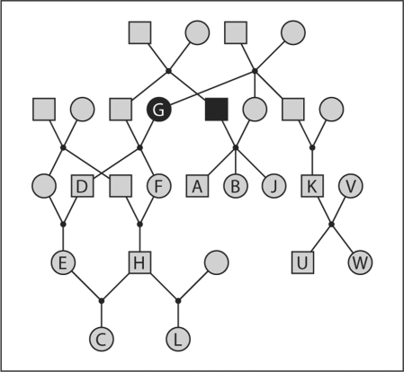
The probability structure of equ. 1, specified through the conditional independence of offspring genotypes given the genotypes of parents, more generally implies that data on disjoint parts of the pedigree are conditionally independent given the genotypes of individuals in a cutset dividing these parts. For example, in figure 1, the two black-shaded individuals form a cutset dividing the left and right parts of the pedigree. Conditional on the genotypes of these two individuals, phenotypes on individuals in the left part of the pedigree are independent of those on individuals on the right. This independence structure led to the computational method of pedigree peeling proposed by Elston and Stewart [5] for simple pedigrees, and soon generalized to arbitrary pedigrees [10] and more complex models [11]. The procedure, now well known in the area of latent-variable problems and graphical models [12], involves the sequential summing out of latent genotypes, and the computational complexity is basically that of the largest number of possible genotype configurations on any cutset in the sequence.

Fig. 1.

Genotypic peeling on pedigree structures. The two black-shaded individuals form a cutset. Conditional on the (phased) genotypes of these two individuals, data on observed individuals A, B, K, V, W, and U in the right half of the pedigree are independent of data on observed individuals D, F, E, H, C, and L in the left half of the pedigree.

The model framework of Elston and Stewart [5] is not restricted to single genetic loci, and Ott [6] very early applied it to two loci, developing the first general-purpose linkage analysis program LIPED for computing linkage lod scores on extended pedigrees. The LIPED program is still in use today, over 35 years later; this must be a record in almost any area of science. As genetic marker maps became more available, the need to consider more than a single marker and a single trait locus arose, and Ott and colleagues developed the LINKAGE software [4].

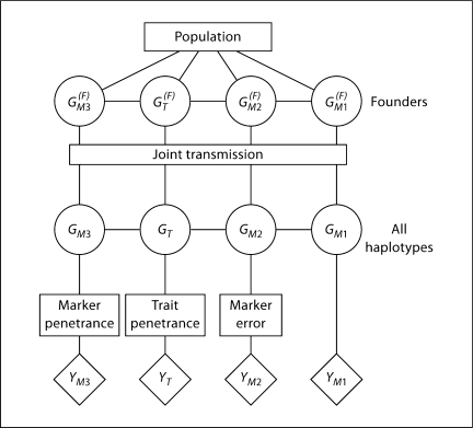
The structure underlying the linkage model and the computation of linkage likelihoods using the LIPED or LINKAGE software is shown in figure 2, for a trait locus and three marker loci. In this and similar figures, models are represented by boxes, latent variables by circles, and observable data by diamonds. For the founder members of the pedigree, the population model specifies the probabilities of the allelic types of DNA and hence also their genotypes. The transmission model specifies the probabilities of meiotic events, and hence the descent of DNA and thence the genotypes of all members of the pedigree. The penetrance model specifies the probability of data observations given the genotype.

Fig. 2.

The genotypic structure of genetic linkage data. The population model provides probabilities of founder haplotypes. The transmission (or meiosis) model then provides probabilities for all haplotypes in the pedigree, and the penetrance model for genetic markers or traits provides probabilities of observable data.

A key feature of the genetic model underlying the LINKAGE software, in which the latent variables are the phased genotypes of individuals, is its generality. The population model provides probabilities for the pair of haplotypes in each founder. Allelic association (LD) can be accommodated as well as departures from the Hardy-Weinberg equilibrium at the population level. Likewise the transmission model is general, allowing not only for different probabilities for different meioses (e.g. different male/female recombination rates) but also for genetic interference. Finally, the penetrance model is general. Although shown in figure 2 as the usually assumed separate model at each locus, in principle this could also be a joint model across loci. Even within each locus, penetrance models are general. For some markers, such as M₁, we may assume genotypes are observed, leading to a deterministic relationship between latent genotype G_M1 and the marker phenotype Y_M1 of any observed individual. However, accommodating a marker error model (e.g. marker M₂) or a more general genotype/phenotype relationship (e.g. marker M₃) is computationally no more intensive. The data observations, Y_T, may be qualitative or quantitative, and the penetrance probability may depend on other covariate information on the individual, such as age, sex, or geographic location.

The disadvantage of the structure of figure 2 is also apparent, in that the latent variables are multilocus haplotypes, and the number of these increase exponentially with the number of loci. Joint analysis of more than a few loci is computationally prohibitive.

From Genotypes to Inheritance

As genetic linkage maps developed and multiple mapped DNA markers became available [13], a new framework was needed for analyses using these multiple marker loci jointly. This was provided by Lander and Green [14], who used indicators of meiosis as the latent variable. For each meiosis i in the pedigree, i = 1, …, m and for multiple loci j along a chromosome, j, j = 1, …, 1, we define

$$\begin{array}{c}{s}_{i,j}\hspace{0.17em}=\hspace{0.17em}0\hspace{0.17em}\text{if DNA transmitted in meiosis}\hspace{0.17em}i\hspace{0.17em}\text{at locus}\hspace{0.17em}j\hspace{0.17em}\text{is parent's maternal DNA}\\ =1\hspace{0.17em}\text{if DNA transmitted in meiosis}\hspace{0.17em}i\hspace{0.17em}\text{at locus}\hspace{0.17em}j\hspace{0.17em}\text{is parent's paternal DNA}.\end{array}$$ (2)

The array S = {S_i,j} now become the latent variables and for convenience we define a meiosis vector, S_i,., for each meiosis and an inheritance vector, S_.,j [14], for each locus:

$$\begin{array}{c}{S}_i,.\hspace{0.17em}=\hspace{0.17em}\left\{S_{i,j};j\hspace{0.17em}=\hspace{0.17em}1,\hspace{0.17em}\mathrm{\dots },\hspace{0.17em}l\right\},\hspace{0.17em}i\hspace{0.17em}=\hspace{0.17em}1,\hspace{0.17em}\mathrm{\dots },\hspace{0.17em}m\\ S.{,}_j\hspace{0.17em}=\hspace{0.17em}\left\{S_{i,j};\hspace{0.17em}i\hspace{0.17em}=\hspace{0.17em}1,\hspace{0.17em}\mathrm{\dots },\hspace{0.17em}m\right\},\hspace{0.17em}j\hspace{0.17em}=\hspace{0.17em}1,\hspace{0.17em}\mathrm{\dots },\hspace{0.17em}l.\end{array}$$

The independence of meioses is equivalent to the independence of vectors S_i,..

At any locus j, the genotypes of individuals are a deterministic function of the allelic types ${\mathcal{A}}_j^{\left(\mathcal{F}\right)}$ of founders $\mathcal{F}$, together with the inheritance vector S_.,j. Hence these variables jointly determine, via a penetrance model, the probabilities of observed phenotypes determined by genotypes at marker or trait locus j. However, in order to place the likelihood in a computationally tractable form, assumptions must be made. First, we assume a Hardy-Weinberg equilibrium and the absence of allelic association (LD): the allelic types of founder genomes are then independent over (haploid) genomes and over loci. Second, we assume the absence of genetic interference; the components of S_i,., and hence inheritance vectors S_.,j, then have a Markov conditional independence structure over loci j. The likelihood becomes

$$P\left(\mathbf{Y}\right)\hspace{0.17em}=\hspace{0.17em}\sum _{\text{S}}\text{P}\left(\mathbf{Y}\hspace{0.17em}|\mathbf{S}\right)\hspace{0.17em}\text{P}\left(\text{S}\right)\hspace{0.17em}=\hspace{0.17em}\sum _{\text{S}}\left[\prod _{j\hspace{0.17em}=\hspace{0.17em}1}^l\hspace{0.17em}\text{P}\left(Y.{,}_j\hspace{0.17em}|S.{,}_j\right)\right]\hspace{0.17em}\text{P}\left(S.{,}_1\right)\left[\prod _{j\hspace{0.17em}=\hspace{0.17em}2}^{l}P\left(S.{,}_j\hspace{0.17em}|S.{,}_{j\hspace{0.17em}-\hspace{0.17em}1}\right)\right]$$ (3)

which maybe compared with equ. 1.

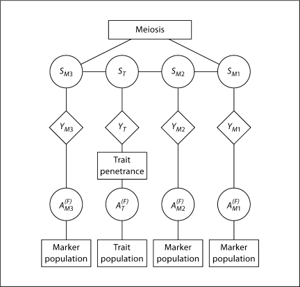
The structure of the problem when S are considered the latent variables is shown in figure 3. The meiosis model becomes primary, providing the probabilities of each meiosis vector S_i,.. The population model provides the allelic types of founder genomes, ${\mathcal{A}}^{\left(\mathcal{F}\right)}$, and the penetrance model relates, at each locus j, the inheritance vector S_.,j and allelic types ${\mathcal{A}}_j^{\left(\mathcal{F}\right)}$ to the data Y_.,j observed on the pedigree. Under the Markov assumption for S_.,j (the absence of genetic interference) and the independence of allelic types across loci (the absence of LD), standard hidden Markov model (HMM) computational methods apply [15]. In fact, since meioses are independent, the structure is that of a factored HMM [16]. Nonetheless, computation is exponential to the number of meioses in the pedigree, and the generality of the model underlying equ. 1 is lost in equ. 3. Additionally there is the requirement, at every locus j, to compute P(Y_.,j | S_.,j) for every inheritance vector S_.,j (see also the next sections).

Fig. 3.

The HMM inheritance structure of genetic linkage data. The meiosis model determines the probabilities of meiosis indicators S which have a Markov dependence over loci. The population model at each locus provides the probabilities of allelic types βf^Tj of founders <F. Then S and β together determine the genotypes of individuals and hence probabilities of phenotypes.

Realization of Inheritance at Marker Loci Given Marker Data

Let Γ denote a specific linkage model for trait data Y_T and marker data Y_M, and let Γ₀ denote the same model but with the absence of linkage between trait and marker loci. The linkage lod score is then

$$\text{lod}\hspace{0.17em}=\hspace{0.17em}{log}_{10}\frac{\text{P}\left({\mathbf{Y}}_T,{\mathbf{Y}}_M;\Gamma \right)}{\text{P}\left({\mathbf{Y}}_T,{\mathbf{Y}}_M{\Gamma }_0\right)}\hspace{0.17em}=\hspace{0.17em}{log}_{10}\frac{\text{P}\left({\mathbf{Y}}_T,{\mathbf{Y}}_M;\Gamma \right)}{\text{P}\left({\mathbf{Y}}_T;\Gamma \right)\text{P}\left({\mathbf{Y}}_M;\Gamma \right)}\hspace{0.17em}=\hspace{0.17em}{log}_{10}\frac{\text{P}\left({\mathbf{Y}}_T|{\mathbf{Y}}_M;\Gamma \right)}{\text{P}\left({\mathbf{Y}}_T;\Gamma \right)}$$ (4)

since the marginal probabilities of Y_M and Y_T are the same under models Γ and Γ₀, and, in the absence of linkage, trait and marker data are independent.

Further partitioning Γ into part Γ_M relating to the marker data Y_M and part γ_T relating to trait data Y_T, we have

$$\text{P}\left({\mathbf{Y}}_T\hspace{0.17em}|{\mathbf{Y}}_M;\Gamma \right)\hspace{0.17em}=\hspace{0.17em}\sum _{{\text{S}}_M}\text{P}\left({\mathbf{Y}}_T\hspace{0.17em}|{\mathbf{S}}_M;{\Gamma }_T\right)\text{P}\left({\mathbf{S}}_M\hspace{0.17em}|{\mathbf{Y}}_M;{\Gamma }_M\right)={\text{E}}_{{\Gamma }_M}\left(\text{P}\left({\mathbf{Y}}_T\hspace{0.17em}|{\mathbf{S}}_M;{\Gamma }_T\right)|{\mathbf{Y}}_M\right).$$ (5)

where S_M denotes the inheritance vectors at all marker locations.

Lange and Sobel [17] used the lod score in the form of equ. 4, and used equ. 5 to develop a Monte Carlo approach to the estimation of linkage lod scores. In this approach Markov chain Monte Carlo (MCMC) is used to sample realizations of S_M conditional on marker data. For each realization, P(Y_T | S_M; Γ_T) is computed by a version of pedigree peeling (equ. 1), in which probabilities of offspring trait-locus genotypes given those of the parents are conditioned on the inheritance vectors at flanking marker loci. These values of P(Y_T | S_M; Γ_T) are averaged over the MCMC realizations to provide a Monte Carlo estimate of P(Y_T | Y_M; Γ) (equ. 5) and hence of the lod score (equ. 4).

Over the last 20 years, there have been several MCMC approaches to the realization of latent inheritance patterns given marker and/or trait data [18, 19, 20, 21, 22]. All approaches include computations following the form of equ. 1 and/or equ. 3 as part of the MCMC sampling process. However, at each stage of sampling, the computations are performed only for a single locus or a small number of meioses. For our current discussion, the approach of Lange and Sobel [17] has several advantages. First, as noted by these authors, for a given marker model MCMC needs to be performed only once. This single set of multiple realizations of S_M provide Monte Carlo estimates of linkage lod scores for multiple trait-locus models and multiple hypothesized trait-locus locations. Second, since the MCMC is performed only to obtain realizations of S_M given the marker data Y_M, the probabilities P(Y_.,j | S_.,j) of equ. 3 are required only for marker loci. For single-locus marker genotypes observed without error, there are very efficient ways to compute this probability [18, 22, 23]. However, this no-error limitation places another restriction on the HMM framework of figure 3 relative to that of the LINKAGE package shown in figure 2.

From Inheritance to Identity-by-Descent

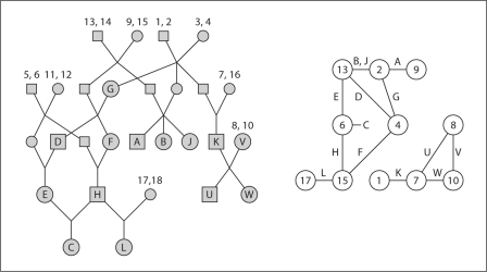
The inheritance vector S_.,j at locus j determines the pattern of gene ibd among observed individuals, and this pattern is key to computation of the probability P(Y_.,j | S_.,j) of observed trait or marker phenotypes. Figure 4 shows again the example pedigree of figure 1, but now with the founder genomes labeled 1 through 18. The larger icons labeled with letters denote observed individuals, and a specific inheritance vector is assumed. Under this inheritance pattern, it is assumed that the observed individuals receive, at this locus, the founder genome indicated in the right-hand graph, the founder-genome-label (FGL) graph. That is, A received 2 and 9, his sisters B and J received 2 and 13, and so on. Individual C received two copies of founder genome labeled 6.

Fig. 4.

The ibd graph as a function of inheritance. The ibd graph (right) shows the FGLs received by the observed individuals in the pedigree (left) under a particular pattern of inheritance.

The probabilities of observed data dependent on genotypes at locus j can be computed using the FGL graph, not only for marker data observed without error [18, 23], but also for any general trait or marker phenotype [22, 24]. We assume only that the allelic types of distinct founder genomes are independent; suppose the allelic type of FGL label k is $\mathcal{A}\left(k\right)$ with population frequency $q\left(\mathcal{A}\left(k\right)\right)$. Suppose also that observed individual i with phenotype Y_i carries FGL k₁(i) and k₂(t). Then the probability of the observed data Y = {Y_i; i observed} is

$$\text{P}\left(\mathbf{Y}\hspace{0.17em}|\text{FGL graph}\right)=\hspace{0.17em}\sum _{\mathcal{A}}\left[\prod _i\text{P}\left({\text{Y}}_i|\mathcal{A}\left(k_1\left(i\right)\right),\mathcal{A}\left(k_2\left(i\right)\right)\right)\right]\left[\coprod _{k}a\left(\mathcal{A}\left(k\right)\right)\right]$$ (6)

where the sum is over all assignments of allelic types to the FGL appearing in the FGL graph.

Equ. 6 may be compared with equ. 1 and 3. All three equations share the same structure of a sum over product terms which involve only a few elements. Precisely the same peeling computations over the graph apply. In fact, since FGL components are usually considerably smaller than the pedigrees from which they derive (see for example the two graphs of fig. 4), computations on the FGL graph are usually considerably faster than on a pedigree. On the other hand, these are conditional probabilities given the FGL graph.

Another feature of the FGL graph is that the founder gene labels are irrelevant. It is the version of the graph with unlabeled nodes that specifies the pattern of ibd among the observed individuals at this locus, and determines the probability of trait phenotypes given the graph (equ. 6). We will refer to the unlabeled version as the ibd graph.

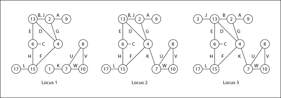
Of course, as we consider different locations along a chromosome, the ibd graph will change as a result of recombination events that change the pattern of ibd among observed individuals. For example, a recombination in the paternal meiosis of individual K (see fig. 4) might give the change in the ibd graph from the previous one shown as locus 1 in figure 5 to that of locus 2. Individual K gains ibd with his aunt G and cousins D and F, and at locus 2 there is one fewer distinct genome present among the observed individuals. Next a recombination in the maternal meiosis of individual J would lead to J no longer sharing both her haplotypes ibd with her sister B, but instead having, as her maternal genome, one not previously present (locus 3 in fig. 5). From locus 2 to locus 3, some ibd is lost, and at locus 3 there is one extra distinct genome present among the observed individuals. Note that in figure 5 the FGL labeling of nodes has been retained. This is for visual clarity only: only the unlabeled ibd graph is required for computation.

Fig. 5.

ibd graphs changing as a result of recombination events. The three graphs show the ibd among the observed individuals (edges labeled with letters), at three loci along the chromosome. Each change is the result of a single recombination event in the ancestry of an observed individual (see text for details).

There are two important features of these changing ibd graphs. The first is that since, in any meiosis, recombination occurs at an average rate of order 10⁻⁸ per base pair (bp), changes in the graph are few. The graph typically remains constant over millions of bp or over several cM. The second is that the disjoint components of the ibd graph are typically small. Thus even when the phenotypes of individuals are affected by genotypes at two loci, or allelic types at four nodes, computation of joint phenotype probabilities (equ. 6) on the combined graph often remains feasible.

Separating Marker and Trait Analyses

As marker data become ever more numerous, inference of inheritance from marker data becomes computationally more challenging. On the other hand, as trait data and models become more complex, trait data themselves contribute little to the inference of this inheritance. Additionally, it may be desirable to analyze multiple traits, and/or multiple trait models, using the same marker data. Thus the formulation of Lange and Sobel [17] separating marker and trait data in the computation of lod scores (equ. 5) becomes the method of choice.

However, we take this separation further, generating patterns of inheritance across the genome from SNP marker data, and outputting these for use in trait analyses. These are generated by the MORGAN-3 program gl_auto [25] which uses the MCMC methods of Tong and Thompson [26] to sample inheritance patterns at all marker locations conditional on all marker data observed in the pedigree data set. The basic output required is a list of realizations of FGL of all individuals at all marker locations across a chromosome. Typically, we generate 1,000 such realizations, sampled at a spacing in the MCMC run such that the realizations are weakly correlated and such that total MCMC run provides good mixing. Clearly, out-putting this information in raw format would be prohibitive. However, most importantly, changes in FGL are few, and only changes need be recorded. Thus each chromosome is output with the initial FGL, the number of changes in FGL, and then a set of pairs indicating the marker or bp location of a change, and the identity of the next FGL. In this format, marker density does not have an impact on the size of the output file, and an output of 1,000 realizations on a sizeable data set is practical. This FGL output then determines the ibd graph, $\mathcal{D}$, at any location on the chromosome.

Where dense markers are used to realize the ibd structure over a chromosome, linkage resolution is such that a computation of lod scores is required only at some (often quite small) subsets of marker locations [27]. At these locations, the ibd structure, $\mathcal{D}$, must be as for that marker. In fact, it is a reduction of that ibd structure, since for the trait computation we require only the ibd graph for individuals O_T observed for trait T. Given the multiple realizations of this ibd structure provided by the gl_auto output, the analysis of trait data can then proceed conditionally only on these realizations.

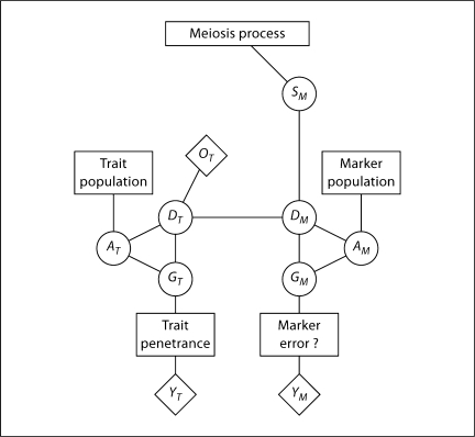
The computation and inference structure becomes that of figure 6, which may be compared with that of figure 3. Again the meiosis process is the prior model for the meiosis indicators S, now considered only at marker loci M. The meiosis indicators at marker loci S_M determine the ibd graph ${\mathcal{D}}_M$ at all marker loci. The marker population model provides probabilities of allelic types ${\mathcal{A}}_M$ at marker loci, and marker haplotypes G_M are determined by ${\mathcal{D}}_M$ and ${\mathcal{A}}_M$. In principle, using the ibd graph computation of equ. 6, a general relationship (e.g. a genotype error model) could be imposed between (phased) marker genotypes G_M and marker phenotypes Y_M. On a genome-wide basis this will not be computationally practical, and standard methods of eliminating aberrant SNPs and clustering SNPs in LD [7] will continue to be used. However, in a small region of the genome of interest, including additional SNPs while allowing an error model may increase the power to detect or resolve linkage. In any event, the right-hand part of the graph permits the realization of S_M and hence ${\mathcal{D}}_M$ conditional on marker data Y_M.

Fig. 6.

Structure of genetic data with modern dense SNP marker data (M) for analysis of trait data T. The right half of the figure shows the structure for realization of ibd graphs (DM at marker locations, conditional on all marker data. The left part shows the structure for analysis of trait data, using the realized (D_M (see text for details).

The left-hand part of figure 6 relates to the trait. The ibd graphs, ${\mathcal{D}}_T$ reduced from the realizations of ${\mathcal{D}}_M$ by restricting to the observed individuals O_T, at any location (s) of hypothesized trait loci are directly put into trait data analyses. The contribution to the lod score for each ${\mathcal{D}}_T$ is again a computation of the form of equ. 6. The trait population model determines probabilities of allelic types ${\mathcal{A}}_T$ which together with ${\mathcal{D}}_T$ determine trait genotypes G_T. These, in turn, via the penetrance model, give probabilities of data Y_T given each ${\mathcal{D}}_T$ and hence given each realization of S_M. These are combined to give a lod score estimate as in the Lange-Sobel approach (equ. 4,5).

Examples of ibd Graph Equivalence

The FGL format described in the previous sections as the output of the MCMC gl_auto program is a compact and easily constructed output of the marker-based MCMC. However, it is not directly well suited to trait data analyses. First, for each particular location, the ibd graph $\mathcal{D}$ must be reconstructed from the FGL change-point information on the two chromosomes of each individual. Second, recall that it is the unlabeled structure of the ibd graph that is relevant to trait data analyses; many apparently different FGL labelings give rise to the same ibd graph. (A small example is given below.) Third, where marker data are informative as to gene ibd among observed individuals, many of the realized ibd graphs may be identical. A method to identify and count the equivalent graphs is required, in order that trait likelihood computations are computed only once for each distinct graph. Finally, particularly on smaller pedigrees, graphs may be constant over a substantial marker range. Where the graph is constant, so is also the trait likelihood contribution under any given trait model, and recomputation is unnecessary for that component pedigree.

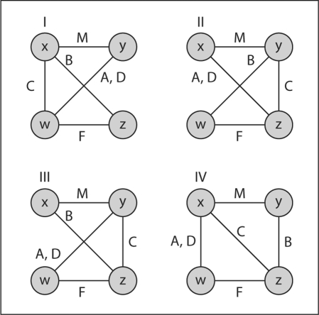
Software has been implemented to determine the ibd graph equivalence over all markers or at a specific marker [28]. This IBDgraph software is described briefly by Koepke in the online supplementary material (www.karger.com/doi/10.1159/000313555) and is also available for download [29]. Figure 7 shows a very small example of ibd graph equivalence. For a nuclear family within the Ped47 pedigree of the example below, the software identified two pairs of graphs as equivalent over a marker range; the figure shows the graphs at only the first marker in the range. The individuals are two parents M, carrying genomes x and y, and F, carrying genomes w and z, and their four offspring A, B, C, and D. It can be seen that graphs I and II are equivalent through the within-parent interchanges x ↔ y and w ↔ z, while III and IV are equivalent through the single interchange x ↔ y. If M and F are unobserved for the trait, only the ibd graph of the four offspring A, B, C and D is relevant. Specifying that only these four individuals are to be included, the IBDgraph software immediately identifies all four graphs as equivalent, since, for example, II is transformed to III via the interchanges x ↔ w and y ↔ z: that is interchange of the now unobserved M and F.

Fig. 7.

Equivalence of ibd graphs under relabeling. When all individuals are observed, graphs I and II are equivalent, as are III and IV. When M and F are unobserved, all four graphs are equivalent.

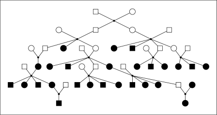
Two examples of the output of the IBDgraph software at single marker locations are summarized in table 1. The first relates to two sets of 1,666 realizations of the FGL output from the gl_auto program run on a 4-generation, 26-member pedigree that is part of a real linkage analysis study (Wijsman, pers. commun.). The second example uses a simulated data set for which the 6-generation 47-member pedigree is shown in figure 8. This pedigree and marker data set is available as part of the MORGAN Tutorial Examples [30]. Ped31 is the 5-generation, 31-member, left-hand part of Ped47, and Pedl4 is the 3-generation, 14-member, right-hand part. For this example, the gl_auto output is a single set of 1,000 FGL realizations. The program was run using the multiple-meiosis sampler [26], and realizations were generated at a spacing of 30 MCMC scans.

Table 1.

Summary of the output of the IBDgraph software at single marker locations, for three outputs of the gl_auto program

Pedigree	Individuals with marker	Individuals in ibd graph	FGL graphs	Equivalence classes	Mean size over FGL	Median size over FGL
Ped26-ChrA	22	26	1,666	24	208.3	218
Ped26-ChrB	18	26	1,666	277	11.2	12
Ped26-ChrB	18	20	1,666	14	648.7	730
Ped47	27	47	1,000	829	1.5	1
Ped47-obs	27	27	1,000	370	8.0	5
Ped31	19	31	1,000	386	6.1	4
Ped31-obs	19	19	1,000	162	21.1	13
Pedl4	8	14	1,000	16	362.0	413
Pedl4-obs	8	8	1,000	10	759.4	865

Two sets of 1,666 realizations were obtained from running gl_auto on Ped26 on two chromosomes here denoted ChrA and ChrB. A single set of 1,000 realizations was obtained from running gl_auto on Ped47. Ped31 and Pedl4 are two subsets of Ped47.

Fig. 8.

Pedigree Ped47 used for the simulated data analysis. The black-shaded individuals are those for whom marker data are available; on these individuals 5% of the marker genotypes are missing at random.

Each row of table 1 results from a single run of the IBDgraph software, which groups the realizations into equivalence classes across the entire chromosome. Each run of the software takes less than 5 s on a MacBook Pro laptop. Shown in table 1 are the results of the IBDgraph software at a marker of interest in Ped26 and at a typical marker location for Ped47. In the first columns of table 1 are the case identifier, the number of individuals on whom marker data are available, and the number of individuals to be included in assessing the ibd graph equivalences. In real-data analyses the latter would be the individuals whose trait data are to be included in the lod score computation. For example, for Ped31 there are marker data on 19 individuals (fig. 8); in the first run of the IBDgraph software all 31 individuals were included in the analysis, and in the second only the 19 for whom marker data were available. Next in table 1 is shown the total number of FGL graphs analyzed (1,666 or 1,000), the number of equivalence classes, and the mean and median size of the equivalence class of a random FGL realization. So, for example, for Ped31 including only the 19 individuals on whom there are marker data, the 1,000 realizations fall into 162 equivalence classes, and the mean and median sizes of the class into which a random one of the 1,000 realizations falls are 21.1 and 13, respectively.

Table 1 shows that, where marker data are informative, the large number of FGL realizations fall into relatively few equivalence classes. For example, for Ped26 on chromosome A where 22 of the 26 individuals have marker data, the 1,666 realizations fall into 24 equivalence classes; at this marker position only 24 lod-score contributions need to be computed. Moreover, the vast majority of the realizations fall into just 8 classes, as can be seen by the mean and median class sizes of >200. If these 8 lod-score contributions comprising 1,645 of the 1,666 realizations show no evidence of linkage, it may even be unnecessary to compute the contributions from the remaining 16 classes (21 total realizations). Unfortunately, on chromosome B, a 6-member branch of Ped26 has no marker data. If the ibd graph is to include all 26 pedigree members, the 1,666 realizations fall into 277 classes, and the typical realization is equivalent to only 10 or 11 others. However, even this provides for an order of magnitude reduction in lod-score computation. Moreover, if the 6-member branch is excluded from the ibd graph assessment, there are only 14 equivalence classes, a reduction of the 1,666 by two orders of magnitude. Also, over 1,460 realizations fall into just 2 classes.

To understand the results more fully, table 1 also shows the results for the 1,000 FGL realizations on Ped47 (fig. 8) at a single typical marker location on the chromosome. Since only 27 members of the pedigree have marker data and there are almost no data on the first three generations, when all 47 individuals are included very few of the ibd graphs are equivalent. There are 829 distinct classes among the 1,000 realizations. Even when the graphs are restricted to the 27 individuals having marker data, there are still 370 classes, with the typical realization being equivalent to only 5–10 others. Relative to Ped26, this reflects the larger number of possible inheritance patterns on this 47-member pedigree, the larger proportion of individuals with no marker data, and the fact that the markers in this simulated data set are less informative than those used in the real-data study (Wijsman, pers. comm.). Even when the ibd graphs are restricted to the 19 observed members of Ped31 (the 31-member left-hand part of Ped47; fig. 8), there are still 162 classes with the typical FGL realization being equivalent to only 20 others on average. However, even this represents an order-of-magnitude reduction in lod-score computational cost. Where pedigrees have less depth, the number of possible inheritance patterns is reduced. For example, for the 3-generation, 14-member, right-hand part of Ped47, we again achieve computational reductions of two orders of magnitude. In fact, when the ibd graphs are restricted to the 8 individuals having marker data, 865 of the 1,000 realizations fall into a single class (table 1).

Overall, we see that for an IBDgraph run taking only a few seconds, we can reduce the subsequent lod-score computational cost by as much as two orders of magnitude. Additionally, trace plots of the equivalence classes of successive FGL realizations can be used to assess the mixing performance of the MCMC with regard to accuracy of lod score estimation. For the examples of this paper, these plots show that the MCMC samples taken at a spacing of 30 scans are well mixed (results not shown). This indicates also that if a user chooses to use more FGL realizations to estimate lod scores, the computational savings of using the IBDgraph software would be even greater. For example, if the length of the MCMC gl_auto run and hence the number of FGL realizations in the first Ped26-ChrA example (table 1) were doubled, a few new ibd graphs might be generated. However, as for the first 1,666 realizations, over 98% of the new FGL realizations will have ibd graphs in one of the 8 major equivalence classes and for these the lod-score contributions are already computed.

In part, the real-data Ped26 example is included to demonstrate the advantages of the approach in terms of data confidentiality. To run the MORGAN gl_auto program, pedigree and marker data are required, but there are no trait data involved. Then, to run the IBDgraph software, no pedigree, marker, or trait data are required. One needs only the indices in the gl_auto output of the subset of the pedigree members whom the researcher wishes to include in their ibd graphs. The researcher may then use the IBDgraph output to significantly reduce the computational costs of their trait-data analyses.

Conclusion

Computation or estimation of linkage lod scores remains a key tool in the genetic mapping of traits. The same principles of conditional independence that underlie the still useful and still used 35-year-old LIPED program [6] extend to linkage computations for current complex traits of interest and to current marker data. However, despite increases in computer speed of the order of millions, computation remains a challenge, since the density of marker data has increased by a comparable factor. Further, the dependence structure of data among markers is a factor that is not relevant for 2-point linkage computations, but is the breaking point for many multipoint approaches.

With increasingly large amounts of marker data, and with trait data that are often complex and do not in themselves provide clear evidence of ibd among relatives, the separation of marker and trait computations in the form first proposed by Lange and Sobel [17] becomes the approach of choice. It enables a single marker-based computation of ibd probabilities, or a single sample of marker-based ibd realizations, to be used for many trait phenotypes, trait models, and hypothesized trait-locus locations.

In our recent software, we have gone further than the within-program separation implied by equ. 5 and used earlier MORGAN lod score programs [25] such as lm_markers [31]. Our new program, gl_auto, analyzes only the marker data, outputting realizations of the FGL of individuals in a compact format where only recombination breakpoints are recorded. Since these are very few for any meiosis and on any chromosome, even for large data sets and (say) 1,000 realizations, the files are man ageable. These output files can then be used for multiple trait analyses. Moreover, since the connected components of the FGL graph are often small, trait analyses for models jointly involving more than a single trait locus become practical.

However, this format is not computationally efficient, particularly when only a subset of the individuals are observed for the trait or when marker data provide clear information about the probable patterns of ibd. Moreover, ibd patterns may remain constant over large chromosome segments on many subcomponents of the overall FGL graph. Where this equivalence of ibd patterns over realizations and their constancy over chromosome segments can be recognized, much recomputation can be avoided. To achieve this, IBDgraph software has been implemented [29], and is described in the online supplementary material. Examples have shown this can reduce subsequent lod-score computational costs by up to two orders of magnitude. This approach of first creating ibd graphs in a compact and efficient format, and then using these in complex trait analyses seems to provide a way forward in the era of dense SNP data and even potentially of sequence data.

References

- 1.Smith CAB. Detection of linkage in human genetics. J R Stat Soc Series B. 1953;15:153–192. [Google Scholar]
- 2.Morton NE. Sequential tests for the detection of linkage. Am J Hum Genet. 1955;7:277–318. [PMC free article] [PubMed] [Google Scholar]
- 3.Ott J. Analysis of Human Genetic Linkage. ed 3. Baltimore: The Johns Hopkins University Press; 1999. [Google Scholar]
- 4.Lathrop GM, Lalouel JM, Julier C, Ott J. Strategies for multilocus linkage analysis in humans. Proc Natl Acad Sci USA. 1984;81:3443–3446. doi: 10.1073/pnas.81.11.3443. [DOI] [PMC free article] [PubMed] [Google Scholar]
- 5.Elston RC, Stewart J. A general model for the analysis of pedigree data. Hum Hered. 1971;21:523–542. doi: 10.1159/000152448. [DOI] [PubMed] [Google Scholar]
- 6.Ott J. Estimation of the recombination frequency in human pedigrees: efficient computation of the likelihood for human linkage studies. Am J Hum Genet. 1974;26:588–597. [PMC free article] [PubMed] [Google Scholar]
- 7.Abecasis G, Wigginton J. Handling marker-marker linkage disequilibrium: pedigree analysis with clustered markers. Am J Hum Genet. 2005;77:754–767. doi: 10.1086/497345. [DOI] [PMC free article] [PubMed] [Google Scholar]
- 8.Thompson EA. MCMC in the analysis of genetic data on related individuals. In: Brooks GJS, Gelman A, Meng XL, editors. Handbook of Markov Chain Monte Carlo. New York: Chapman & Hall/CRC Press; 2011. in press. [Google Scholar]
- 9.Haldane JBS, Smith CAB. A new estimate of the linkage between the genes for colour-blindness and haemophilia in man. Ann Eugen. 1947;14:10–31. doi: 10.1111/j.1469-1809.1947.tb02374.x. [DOI] [PubMed] [Google Scholar]
- 10.Cannings C, Thompson EA, Skolnick MH. Probability functions on complex pedigrees. Adv Appl Proby. 1978;10:26–61. [Google Scholar]
- 11.Cannings C, Thompson EA, Skolnick MH. Pedigree analysis of complex models. In: Mielke J, Crawford M, editors. Current Developments in Anthropological Genetics. New York: Plenum Press; 1980. pp. 251–298. [Google Scholar]
- 12.Lauritzen SJ. Propagation of probabilities, means and variances in mixed graphical association models. J Am Stat Assoc. 1992;87:1098–1108. [Google Scholar]
- 13.Botstein D, White RL, Skolnick MH, Davis RW. Construction of a linkage map in man using restriction fragment polymorphism. Am J Hum Genet. 1980;32:314–331. [PMC free article] [PubMed] [Google Scholar]
- 14.Lander ES, Green P. Construction of multilocus genetic linkage maps in humans. Proc Natl Acad Sci USA. 1987;84:2363–2367. doi: 10.1073/pnas.84.8.2363. [DOI] [PMC free article] [PubMed] [Google Scholar]
- 15.Baum LE, Petrie T, Soules G, Weiss N. A maximization technique occurring in the statistical analysis of probabilistic functions on Markov chains. Ann Math Stat. 1970;41:164–171. [Google Scholar]
- 16.Fishelson M, Geiger D. Optimizing exact linkage computations. J Comput Biol. 2004;11:263–275. doi: 10.1089/1066527041410409. [DOI] [PubMed] [Google Scholar]
- 17.Lange K, Sobel E. A random walk method for computing genetic location scores. Am J Hum Genet. 1991;49:1320–1334. [PMC free article] [PubMed] [Google Scholar]
- 18.Sobel E, Lange K. Descent graphs in pedigree analysis: applications to haplotyping, location scores, and marker-sharing statistics. Am J Hum Genet. 1996;58:1323–1337. [PMC free article] [PubMed] [Google Scholar]
- 19.Heath SC. Markov chain Monte Carlo segregation and linkage analysis for oligogenic models. Am J Hum Genet. 1997;61:748–760. doi: 10.1086/515506. [DOI] [PMC free article] [PubMed] [Google Scholar]
- 20.Thompson EA. Statistical Inferences from Genetic Data on Pedigrees, vol. 6. NSF-CBMS Regional Conference Series in Probability and Statistics. Beachwood: Institute of Mathematical Statistics; 2000. [Google Scholar]
- 21.George AW, Thompson EA. Multipoint linkage analyses for disease mapping in extended pedigrees: a Markov chain Monte Carlo approach. Stat Sci. 2003;18:515–531. [Google Scholar]
- 22.Thompson EA. MCMC in the analysis of genetic data on pedigrees. In: Liang F, Wang JS, Kendall W, editors. Markov Chain Monte Carlo: Innovations and Applications. Singapore: World Scientific Co Pte Ltd; 2005. pp. 183–216. [Google Scholar]
- 23.Kruglyak L, Daly MJ, Reeve-Daly MP, Lander ES. Parametric and nonparametric linkage analysis:a unified multipoint approach. Am J Hum Genet. 1996;58:1347–1363. [PMC free article] [PubMed] [Google Scholar]
- 24.Thompson EA, Heath SC. Estimation of conditional multilocus gene identity among relatives. In: Seillier-Moiseiwitsch F, editor. Statistics in Molecular Biology and Genetics: Selected Proceedings of a 1997 Joint AMS-IMS-SIAM Summer Conference on Statistics in Molecular Biology, IMS Lecture Note – Monograph Series. vol 33. Hayward: Institute of Mathematical Statistics; 1999. pp. 95–113. [Google Scholar]
- 25.MORGAN:a package for Markov chain Monte Carlo in Genetic Analysis (version 3.0). http://www.stat.washington.edu/thompson/Genepi/MORGAN/Morgan.shtml, 2009.
- 26.Tong L, Thompson EA. Multilocus lod scores in large pedigrees: combination of exact and approximate calculations. Hum Hered. 2008;65:142–153. doi: 10.1159/000109731. [DOI] [PMC free article] [PubMed] [Google Scholar]
- 27.Boehnke M. Limits of resolution of genetic linkage studies: implications for the positional cloning of human disease genes. Am J Hum Genet. 1994;55:379–390. [PMC free article] [PubMed] [Google Scholar]
- 28.Koepke HA, Thompson EA. Efficient testing operations on dynamic graph structures using strong hash functions. Technical Report 567. Department of Statistics, University of Washington; 2010. available at www.stat.washington.edu/research/reports/2010/tr567.pdf. [Google Scholar]
- 29.IBDgraph:an add-on for MORGAN 3. http://www.stat.washington.edu/thompson/Genepi/MORGAN/ibdgraph.tar.gz, 2010.
- 30.MORGAN Online Tutorial and Examples (for MORGAN 2.9). http://www.stat.washington.edu/thompson/Genepi/MORGAN/morgan-tut-html-v29/morgan-tut4.html, 2009.
- 31.Wijsman EM, Rothstein JH, Thompson EA. Multipoint linkage analysis with many multiallelic or dense diallelic markers: MCMC provides practical approaches for genome scans on general pedigrees. Am J Hum Genet. 2006;79:846–858. doi: 10.1086/508472. [DOI] [PMC free article] [PubMed] [Google Scholar]