Varying coefficient model for gene–environment interaction: a non-linear look

Abstract

Motivation: The genetic basis of complex traits often involves the function of multiple genetic factors, their interactions and the interaction between the genetic and environmental factors. Gene–environment (G×E) interaction is considered pivotal in determining trait variations and susceptibility of many genetic disorders such as neurodegenerative diseases or mental disorders. Regression-based methods assuming a linear relationship between a disease response and the genetic and environmental factors as well as their interaction is the commonly used approach in detecting G×E interaction. The linearity assumption, however, could be easily violated due to non-linear genetic penetrance which induces non-linear G×E interaction.

Results: In this work, we propose to relax the linear G×E assumption and allow for non-linear G×E interaction under a varying coefficient model framework. We propose to estimate the varying coefficients with regression spline technique. The model allows one to assess the non-linear penetrance of a genetic variant under different environmental stimuli, therefore help us to gain novel insights into the etiology of a complex disease. Several statistical tests are proposed for a complete dissection of G×E interaction. A wild bootstrap method is adopted to assess the statistical significance. Both simulation and real data analysis demonstrate the power and utility of the proposed method. Our method provides a powerful and testable framework for assessing non-linear G×E interaction.

Contact: cui@stt.msu.edu

Supplementary information: Supplementary data are available at Bioinformatics online.

1 INTRODUCTION

The genetic basis of a complex trait often involves multiple genetic factors functioning in a coordinated manner. The extent on how our genetic blueprint expresses also depends on the interactions between genetic and environmental factors. Increasing evidences have shown that gene–environment (G×E) interactions play pivotal roles in determining the risk of diseases, for instance, the psychiatric diseases (reviewed in Caspi and Moffitt, 2006), the neurodegenerative and cardiovascular diseases (Costa and Eaton, 2006), and cancer (Ulrich et al., 1999). Due to the complex nature of the form and mechanism of G×E interaction in different living organisms, hunting down the molecular machinery of G×E interaction has been a daunting task in the post-genomic era. There is a pressing need in developing efficient and powerful statistical methods for a rigorous investigation of G×E interaction.

G×E interaction refers to how genotypes influence phenotypes differently in different environments (Falconer, 1952). From a biological point of view, G×E interaction can be better viewed as the genetic responses to environment changes or stresses (Hoffmann and Parsons,1991; McClintock, 1984). In a typical G×E interaction study design, environment is often defined as different conditions coded as a discrete variable in a statistical model. For example, in a study of G×E interaction related to lung cancer, smoking status can be defined as an environment condition coded as 1 (smoking) or 0 (no smoking). In many other studies, the environment condition is defined as a continuous measure. For one example, studies show that ~80% of type II diabetes and 70% of cardiovascular disease are related to obesity [defined by body mass index (BMI)]. To track down genetic factors responsible for diabetes or cardiovascular disease, obesity can be defined as an environment factor that may induce or reduce the expression of particular genes to affect the disease status. The contribution of the same gene to a disease status may be largely different under different BMI levels. As another example, the peak bone mineral density (BMD) in adulthood varies a lot across different age groups. The amount of nutrition intake (e.g. vitamin D) is also an important environment factor influencing the variation of BMD (Peacock et al., 2002). Individuals carrying the same gene may respond differently to the rate of density decrease as they get older. Also the peak BMD measure may vary a lot across groups with different nutrition intake, potentially due to the interaction of specific genes with the amount of nutrition intake (e.g. vitamin D).

Statistical methods for testing G×E interaction can be broadly categorized into two areas: the model-based method, either parametrically, non-parametrically or semi-parametrically (e.g. Chatterjee and Carroll 2005; Guo 2000; Kraft et al.,. 2007; Maity et al.,. 2009), and the model-free method such as the multifactor dimensionality reduction method (Hahn et al., 2003). In a model-based regression framework, traditional parametric methods need strong model assumptions such as assuming linear G×E interaction as given in model (1). This assumption, however, could be easily violated due to the underlying nonlinear machinery between the genetic and environment factors. Mis-specification in parametric models could lead to large bias. Non-parametric modeling as an alternative way reduces modeling bias by imposing no specific model structure and enables people to explore the data more flexibly at the cost of interpretability. The information about the relationship between the dependent and independent variables from the estimates is often difficult to interpret. Moreover, the variances of the resulting estimates tend to be unacceptably large when the dimension of the covariates is high, which is the so-called ‘curse of dimensionality’. To overcome these difficulties, many different semi-parametric models have been proposed and developed, among which varying coefficient (VC) models have gained considerable attention in recent years and are becoming very popular in data analysis, see for example, the work of Cleveland et al. (1991), Hastie and Tibshirani (1993), Hoover et al. (1998), Fan and Zhang (1999), Cai et al. (2000), Fan and Zhang (2000), Huang et al. (2004) among others. VC models as natural extensions of linear models allow the coefficients to change smoothly with the value of other variables so that one can explore dynamic feature of datasets successfully with good interpretability and flexibility. See Fan and Zhang (2008) for a detailed review. In this article, we apply varying coefficient models to investigate G×E interactions.

In G×E interaction problems, one is interested in understanding how genes respond differently across different environment conditions in determining the variation of a trait or the risk of a disease. We focus our attention to environment conditions measured on a continuous scale. From a statistical point of view, ‘interaction’ is typically modeled as a product term. A simple model to detect interaction would be a simple linear regression model with the form

(1)

where Y is the phenotypic response; α₀ is the overall mean; α₁ and β₁ are the effects of the environment (X) and genetic (G) variables, respectively; β₂ is the effect for G×E interaction; and ε is the error term with mean 0 and variance σ². A simple rearrangement of model (1) leads to

(2)

With this representation, it is clear that the contribution of a gene to the variation of a phenotype Y is restricted to a linear function in X. The form and pattern of the responses are typically unknown and may not follow a linear relationship as described in model (1).

In addressing the limitation of the linear model assumption in dissecting the role of a gene under different environment conditions, one can relax the linearity assumption of G×E interaction and allow for a non-linear interaction by replacing the linear G×E interaction coefficient β₁+β₂X in model (2) by a smooth non-linear function β(X) and apply a VC model to detect non-linear G×E interaction. A VC model has the form

(3)

for given covariates (X,G)^T and the response Y with E(ε|X,G)=0 and Var(ε|X,G)=1. β(X) is a smoothing function in X and σ²(X)=Var(Y|X,G) is the conditional variance function. Under the VC modeling framework, the effect of a gene is allowed to vary as a function of environmental factors, either linearly or non-linearly, captured by the model itself. Thus, the VC model has the potential to dissect the non-linear penetrance of genetic variants.

Methods for the estimation of VC models have flourished in the literature, which can be grouped into three categories. One is local polynomial kernel smoothing, see Fan and Zhang (1999), Xia and Li (1999) and Cai et al. (2000). One is spline-based method, see Huang et al. (2004) for polynomial spline, and Hoover et al. (1998) and Chiang et al. (2001) for smoothing spline. The last one is wavelet estimation, see Zhou and You (2004). In this work, we adopt the polynomial spline approach in Huang et al. (2004) to estimate the coefficient functions β(·) for several major reasons. First, the coefficient functions are approximated by a linear combination of B-spline basis functions, which provides a simple global solution to estimation and inference for VC models, and great flexibility is achieved by using different basis expansions for approximating different coefficient functions, which are stated in Huang et al. (2004). Secondly, because of its global nature in computation, B-splines are computationally expedient compared with kernel-based methods, which is much necessary for analyzing high-dimensional genetic data with hundreds of thousands of markers. Moreover, it is theoretically reliable guarded by the asymptotic consistency and normality property of the spline estimator , see Huang et al. (2004).

Besides estimation, to test whether the coefficient function of β(X) in model (3) is significantly different from zero or a constant or has a presumed parametric form is also of our interest. Because of the distribution-free nature of semi-parametric models, the likelihood ratio test for traditional parametric models cannot be applied. We adopt the wild bootstrapping approach as in Härdle and Mammen (1993) to assess the significance of the tests. The integrated squared difference between the parametric and the non-parametric functional estimates is used as a test statistic, and the critical value is determined by the bootstrap method described in Härdle and Mammen (1993).

The article is organized as follows. In Section 2, we introduce the methodology of applying VC models to genetic data to detect G×E interaction. We introduce the B-spline fitting technique and its necessary notations. We introduce the test statistics for the hypothesis testing evaluated by the wild bootstrap strategy. In Section 3, we study the finite sample properties of the proposed procedure using the simulated example. Furthermore, the utility of the method is illustrated through the analysis of a real dataset detailed in Section 4, followed by the discussion in Section 5.

2 STATISTICAL METHODS

2.1 A two-parameter VC model

In model (3), we only consider the additive effect of a genetic variant. In real life, we do not know the true gene action mode, hence a more flexible model is to consider both additive and dominance penetrance effects. We assume a continuous response variable Y which is a function of an environment variable X and the additive and dominance scales G₁ and G₂ of a genetic factor. Each genetic factor has three possible genotype categories represented by AA, Aa and aa. The three genotype categories can be coded as 1, 0 and −1 for the additive scale G₁ , and as −1/2, 1/2 and −1/2 for the dominance scale G₂, corresponding to genotypes AA, Aa and aa, respectively. We assume allele A is the minor allele with its frequency represented by p_A. We model the coefficients of G₁∈(1,0,−1) and G₂∈(−1/2,1/2,−1/2) for each genetic factor as smooth functions of the environment variable X. Since our major interests are the estimation and inference about the coefficient functions for G₁ and G₂, for simplicity we impose a linear structure on the intercept function α(X) defined in model (3) by letting α(X)=α₀+α₁X, although a non-parametric smooth function can also be fitted. Thus, the redefined VC model is given as

(4)

for given covariates (X,G₁,G₂), with E(ε|X,G₁,G₂)=0, Var(ε|X,G₁,G₂)=1 and the conditional mean function of Y given X, G₁ and G₂ is E(Y|X,G₁,G₂)=m(X,G₁,G₂)=α₀+α₁(X)+β₁(X)G₁+β₂(X)G₂. The same model is fitted separately for each marker, followed by multiple testing corrections. The two-parameter model given in (4) is not only biologically more meaningful than the one-parameter model given in (3), but also statistically attractive since it is invariant to allele coding (i.e. whether code AA as 1 or code aa as 1 for variable G₁).

Remark: varying coefficient models can be considered as locally linear models. By assuming specific expressions for β₁(·) and β₂(·) , model (4) would become a parametric model. For example, by letting β₁(X)=β₁+β₃X, and β₂(X)=β₂+β₄X, where β₁, β₂ , β₃ and β₄ are constants, model (4) can be written as

(5)

which is a linear regression model with main effects for X and (G₁,G₂) as well as their interaction effects (denoted hereafter as LM-I). If we assume a homogeneous residual variance, this is the commonly applied linear regression model for testing G×E interaction which reduces to model (1) if only additive effect is considered. If we impose a constant structure on β₁(X) and β₂(X), i.e. β₁(X)=β₁ and β₂(X)=β₂, then model (4) is reduced to

(6)

which is a linear regression model without the interaction terms (denoted hereafter as LM). Therefore, the traditional linear regression model for testing G×E interaction is a special case of model (4).

Although, their properties are very well established, the conventional parametric approaches are infeasible in this case, since the functional forms of β₁(·) and β₂(·) are unknown to us due to the complexity of the underlying interaction mechanism. Any mis-specification of the model would lead to uncertainty estimates and low power (see Fig. 1 in Section 3 Monte Carlo simulation). By relaxing the linear assumption for the coefficients β₁(X) and β₂(X), model (4) has much flexibility to capture the non-linear penetrance of a genetic variant under different environmental stimuli, thus ensures the power of the proposed VC model in detecting non-linear G×E interactions. In this article, we apply the B-spline smoothing technique to estimate β₁(·) and β₂(·), which solves only one least squares problem to get the estimators. The great advantages of B-spline estimation are simple implementation and fast computation.

Fig. 1.

The power plot under different sample sizes and heritability levels for the three methods. Data were generated with the VC model and were analyzed with the VC, LM and LM-I models.

As in most works on non-parametric smoothing, estimation of the functional coefficients β₁(·) and β₂(·) is conducted on a compact interval [a,b]. In this article, we denote the space of p-th order smooth function on [a,b] as C^(p)[a,b]={g|g^(p)∈C[a,b]}, and C[a,b] is the space of continuous functions on [a,b].

We make the following assumptions on the functional coefficient model, where Assumptions (A1)–(A3) are identical with (A1), (A4) and (A5) in Härdle and Mammen (1993), while Assumption (A4) is the same as (A1) in Wang and Yang (2009):

• (A1) The marginal density f(·) of X is bounded away from zero and f(·)∈C[a,b].

• (A2) σ²(·)=Var(Y|X=x,G) is bounded away from 0 and ∞.

• (A3) E[exp(tε)] is bounded for |t| small enough.

• (A4) For k=1,2,β_k(x)∈C^(q)[a,b], for a given integer q≥1, and the spline order p satisfies p≥q.

2.2 Parameter estimation

Given a random sample {(X_i,G_i,Y_i)}_i=1ⁿ from model (4), the polynomial spline modeling is adopted to estimate β(·). Let _n be the space of polynomial splines of order p≥1. We introduce a knot sequence with N_n interior knots

where N≡N_n increases when sample size n increases, and the precise order is given in Assumption (A5). Then _n consists of functions ϖ satisfying (i) ϖ is a polynomial of degree p−1 on each of the subintervals I_s=[k_s,k_s+1), s=0,…,N_n−1, I_Nn=[k_Nn,b]; and (ii) for p≥2, ϖ is p−2 time continuously differentiable on [a,b]. Let J_n=N_n+p, where N_n is the number of interior knots. We define the normalized B-spline basis as {B_s:1≤s≤J_n}^T as given in Wang and Yang (2009). Equally spaced knots are used in this article for simplicity. The distance between neighboring interior or boundary knots is h=h_n=(b−a)(N_n+1.)⁻¹. For positive numbers a_n and b_n and for n≥1, let a_n~b_n mean that lim_n→∞a_n/b_n=c, where c is some non-zero constant. The number of interior knots satisfy Assumption (A5) below.

• (A5) The number of interior knots N=N_n~n^1/(2p+1), i.e. c_Nn^1/(2p+1)≤N≤C_Nn^1/(2p+1) for some positive constants c_N and C_N.

For each marker, and k=1,2, the coefficients β_k(x) is estimated by where the coefficients are solutions of the following least squares problem

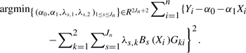(7)

2.3 Number of knots N and spline order p selection

For the proposed model, it is necessary to select appropriate knots and spline order to avoid over- and undersmoothing. For simplicity, we assume the same spline basis {B_s:1≤s≤J_n}^T to approximate the coefficient functions β₁(x) and β₂(x), even though the spline order and knots can be different for the two functions. We use the Bayesian information criterion (BIC) criteria to select the ‘optimal’ N, denoted by , from 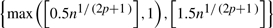, where [b] denotes an integer part of b, and the ‘optimal’ order p for the spline basis, denoted by , from (3,4), which minimize the BIC value , where . p=3 and 4 are the orders for quadratic and cubic splines, respectively. A grid search for the combination of hypothesized values for N and p can be done and the values of N and p corresponding to the minimum of the BIC values are the ‘optimal’ results.

2.4 Hypothesis testing

Before we test possible G×E interaction, the first step is to assess whether a genetic marker is associated with a phenotype. This can be done by formulating the hypotheses

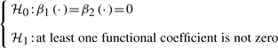(8)

If the null is rejected, then we test significance of the additive effect (G₁) and the dominance effect (G₂), by formulating the hypotheses

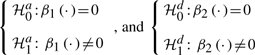(9)

When either the null in (9) is rejected, we then test if the coefficient functions β₁(X) and β₂(X) in model (4) are varying or not. The hypotheses for this test are formulated by

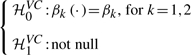(10)

where β_k, k=1,2, are unknown constants, for the selected genetic markers from the first step. Under ₀^VC, the reduced model can be written as Y=α₀+α₁X+β₁G₁+β₂G₂+σ(X)ε, which implies that there is no G×E interaction. Thus, Hypothesis (10) is essentially a test for G×E interaction. Upon rejecting the null, one can also proceed to test ₀^L: β₁(X)=β₁+β₃X and β₂(X)=β₂+β₄X. Under ₀^L, the reduced models can be written as Y=α₀+α₁X+β₁G₁+β₂G₂+β₃G₁X+β₄G₂X+σ(X)ε, a model commonly applied for assessing linear G×E interaction assuming both additive and dominance effects. Rejecting the null implies non-linear G×E interaction.

2.5 Wild bootstrap to assess statistical significance

Note that the current model does not assume any specific distribution for the error term ε , thus there is no likelihood function for the data. Borrowing the idea from Härdle and Mammen (1993), we use the integrated squared deviation between the estimators denoted by and of m(X,G₁,G₂) for the full and reduced models as the test statistic, which would be , where {(X_i,G_1i,G_2i,Y_i),i=1,…,n} is a random sample of (X,G₁,G₂,Y). For the superiority of _n over other goodness-of-fit tests, see the discussion in Härdle and Mammen (1993). The authors pointed out that a way of computing critical values could possibly be based on resampling from the entire dataset. However, it was shown that this bootstrapping method (the classical bootstrap) failed, since the bootstrapped statistic does not have the same limit behavior. Thus, a new variant of the bootstrap method called wild bootstrap was proposed, which is adopted in this work.

For the i-th observation, recall that and are the estimators of m(X_i,G_1i,G_2i) for the reduced and full model, respectively. As discussed in Härdle and Mammen (1993), in order to mimic the i.i.d. structure of (X_i,G_1i,G_2i,Y_i), we need to construct the bootstrap procedure so that , where {(X_i^*,G_1i^*,G_2i^*,Y_i^*)}_i=1ⁿ is the bootstrap sample drawn from the set {(X_i,G_1i,G_2i,Y_i)}_i=1ⁿ. For this purpose, we define and construct , where U_i is a two-point distributed random variable independent of (X_i,G_1i,G_2i,Y_i) satisfying with probability , with probability . By simple calculation, we obtain that E(ε_i^*|X_i,G_1i,G_2i)=0, and . Then we use as bootstrap observations and create ^*,W like _n by the squared deviation between the coefficient estimators under ₀ and ₁. From the Monte Carlo approximation of *(_l^*,W)=(^*,W|(X_i,G_1i,G_2i)_i=1ⁿ), then the P−value p_v is obtained by finding the (1−p_v)-th quantile which satisfies . Multiple testing should be then adjusted among the tests for all markers using a method such as the false discovery rate (FDR) procedure (Benjamini and Hochberg, 1995).

3 MONTE CARLO SIMULATION

A continuous environment measure (e.g. age, diet and body mass), denoted as X, was generated from a normal distribution. Then we transformed X by Z=Φ{(X−μ_X)/σ_X} in order to make X distributed more evenly on each subinterval I_s, where μ_X and σ_X are the mean and SD of X, estimated by the sample mean and SD, and Φ(·) is the cumulative distribution function for the standard normal. We then used the transformed Z to generate the B-spline basis. For k=1,2,β_k(x) was estimated by where the coefficients are solutions of the least squares problem given in Equation (7).

Given a minor allele frequency (MAF) of p_A and assuming Hardy–Weinberg equilibrium, SNP genotypes (AA, Aa and aa) were simulated from a multinomial distribution with frequency (p_A²,2p_A(1−p_A),(1−p_A)²) for (AA, Aa, aa). The genetic variables G_1i and G_2i were coded as (1,0,−1) and () for genotypes (AA, Aa, aa), respectively, following an orthogonal quantitative genetic model (Cockerham, 1954). The random error term ε_i was simulated from N(0,1). Different sample sizes (i.e., n=200, 500, 1000), and different heritability levels (i.e., H²=0.01,0.03,0.05) were assumed. For a given genetic effect and a heritability level, σ(X_i) varies for different X_i, and detailed calculation can be found in the following sections. Data were simulated assuming different gene action modes and were subsequently analyzed by three models, i.e., the proposed VC model, the linear regression model without interaction (denoted as LM), and the linear regression model with interaction (denoted as LM-I). The likelihood ratio test was applied to evaluate the power for testing ₀: β₁=β₂=0 for the LM model and ₀: β₁=β₂=β₃=β₄=0 for the LM-I model. The likelihood ratio statistics follows a chi-square distribution with 2 and 4 degrees of freedom for the two models. Wild bootstrap was applied to assess the test significance of the VC model.

We generated the phenotype data assuming the following VC model

where α₀=3.0, α₁=0.1 and β₁(x) and β₂(x) were generated from the B-spline basis functions such that β₁(x)=∑_s=1⁴λ_1sB_s(x) and β₂(x)=∑_s=1⁴λ_2sB_s(x), in which λ₁₁=−0.53, λ₁₂=0.31 λ₁₃=−0.44, λ₁₄=0.50 , λ₂₁=−0.87, λ₂₂=0.71, λ₂₃=−1.27 and λ₂₄=1.15. These spline coefficients were calculated from Equation (7) based on SNP 22 265 753 from a real dataset (Table 1). The reason we generated β(X) this way is to mimic real data, even though we could generate β(X) from a parametric function such as a sin or a polynomial function. The variance function σ²(x) was obtained by solving H²=V_G/(V_G+V_E), where H² is the heritability level; V_G(x)=β₁²(x)var(G₁)+β₂²(x)var(G₂)+2β₁(x)β₂(x)cov(G₁,G₂) is the genetic variance in which var(G₁)=2p_A(1−p_A), var(G₂)=1/4{1−(2p_A−1)⁴} , and cov(G₁,G₂)=2p_A(1−p_A)(2p_A−1); and V_E=σ²(x). Simple algebra shows that H²=[1+σ²(x)/V_G(x)]⁻¹, which gives σ²(x)=(1/H²−1)V_G(x). Assuming different heritability levels, i.e. H²=0.01, 0.03, 0.05, the phenotype Y_i can be generated assuming ε_i~N(0,1). As can be seen that the genetic variance is a function of the MAF, so does for the residual variance σ(X). For a fixed MAF, the residual variance decreases as the heritability increases. Thus, we expect high power under high H² value. However, due to the way we defined the calculation of V_G, it is no longer true that σ(X) decreases as the MAF increases for a fixed H² level. So the power no longer monotonically increases with the increase of the MAF as usually assumed in human genetic association studies. Based on the estimated frequency (p_A=0.08) of the SNP from the real data, we fixed the allele frequency and evaluated the power performance of the three methods under different heritability levels. Empirical power was recorded based on 1000 simulation repetitions, each with 10 000 bootstrapped samples.

Table 1.

The lists of SNPs with P<0.005 when fitting the data with three different models (VC, LM and LM-I)

SNP ID	Gene name	Location	P_VC	P_const	P_linear	P_LM	P_LMi	P_i
Fitted with VC model
rs8178750*	PLAT	Intron 6a	1E−05	<1E−05	3E−05	0.8827	0.0823	0.0182
rs9622979	PDGFB	Intron 2	0.0008	0.0034	0.0056	0.0655	0.0471	0.1237
rs11701	ANG	Exon 1	0.0013	0.0041	0.0156	0.0930	0.0477	0.0883
rs17876032	F12	Intron 10	0.0018	0.0071	0.0074	0.0234	0.0070	0.0369
634043245a	FGF4	Exon 3	0.0019	0.0046	0.0016	0.0808	0.1452	0.4070
rs12722477	HLA-G	Exon 3	0.0020	0.0120	0.0239	0.0089	0.0029	0.0360
rs2301643	COL1A2	Intron 28	0.0024	0.0103	0.0038	0.0182	0.0222	0.1811
rs2242213	FLT4	Intron 13	0.0027	0.0017	0.0452	0.4106	0.0090	0.0028
rs383483	IL12RB1	Intron 15	0.0027	0.0011	9E−05	0.8376	0.5946	0.2968
rs2521206	COL1A2	Intron 19	0.0038	0.0254	0.0381	0.0148	0.0066	0.0544
rs5743836	TLR9	Promoter	0.0048	0.0243	0.1250	0.0061	0.0053	0.1040
Fitted with LM model
rs1143634	IL1B	Exon 5	0.0053	0.1818	–	0.0006	–	–
rs3783550	IL1A	Intron 6	0.0213	0.629	–	0.0007	–	–
rs17231534	CETP	Intron 1	0.0056	0.2073	–	0.0020	–	–
Fitted with LM-I model
rs2069882*	IL9	Intron 4	0.0024	0.0477	0.4773	0.0009	4.9E−05	0.0039
rs16944	IL1B	Promoter	0.0011	0.0019	0.2477	0.0899	0.0005	0.0005
rs3740938	MMP8	Exon 6	0.0014	0.0009	0.1249	0.4743	0.0009	0.0002
rs9332607	F5	Exon 13	0.0038	0.0237	0.0965	0.0178	0.0032	0.0201
rs439154	IL1RN	Intron 2	0.0314	0.0136	0.4848	0.9035	0.0041	0.0005
rs2296849	COL4A2	Intron 37	0.0154	0.013	0.1005	0.2072	0.0044	0.0025

^aSNP not in dbSNP. Note: P_VC is the P-value for testing hypothesis (8); P_const is the P-value for testing hypothesis (10); P_linear is the P-value for testing linear coefficient (₀^L); P_LM is the P−value for testing ₀: β₁=β₂=0 for fitting a linear model without interaction; P_LMi is the P-value for testing a genetic effect when fitting a linear model with interaction [model (5)], i.e. ₀: β₁=β₂=β₃=β₄=0; P_i is the P-value for testing ₀: β₃=β₄=0 with model (5), a 2 df likelihood ratio test. SNPs shown significance after the FDR control method (Benjamini and Hochberg, 1995) are indicated by *.

Figure 1 shows that the testing power increases as the sample size n and heritability level H² increase for the three models. For a fixed genetic effect, large heritability level leads to small residual variance, and consequently leads to increased power. It is clear that the VC model outperforms the other two models in all cases. Since the linear model with interaction (LM-I) is closer to the VC model in structure, it achieves higher power than the linear model without interaction (LM). The simulation results indicate that when the nature of the G×E interaction is non-linear, i.e. when a variant shows a strong non-linear penetrance effect, a mis-specification of an analytical model assuming a linear structure suffers tremendously from power loss.

We also evaluated the performance of the VC model when the underlying true interaction follows a linear structure or no interaction at all. False positive control of the methods were also studied (see Supplementary Material). Here, we provide a summary of the simulation: (i) when the underlying true interaction model is non-linear, the proposed VC model has the highest power among the three. The other two parametric linear models suffer tremendously from power loss (Fig. 1); (ii) when the underlying true model is linear with or without interaction, the linear model assuming interaction or no interaction has the best power. However, as the sample size and heritability level increase, the power difference between the VC model and the other two decreases significantly; and (iii) in real data analysis, the VC model cannot substitute the other two models before we know the true functional effect. We can first do a hypothesis testing to check if the coefficient functions β_k(X), k=1,2, are constant or linear in X, then apply the optimal model in the analysis. The non-linear VC model would be the choice if the constant or linear function is rejected. Otherwise, a linear model is suggested, especially when sample size is small.

4 REAL DATA ANALYSIS

We applied the method to a real dataset which contains 1536 new born babies, recruited through the Department of Obstetrics and Gynecology at Sotero del Rio Hospital in Puente Alto, Chile. Total 648 single nucleotide polymorphisms (SNPs) covering 189 unique genes were analyzed after eliminating SNPs with MAF <0.05 and those departure from Hardy–Weinberg equilibrium. When fitting to the VC model, we found that the spline design matrix could be singular when there are extremely unbalanced genotype distributions, especially when only two genotypes categories were present for an SNP. Thus, we eliminated additional 143 SNPs and only 505 SNPs were included in our analysis. (Note that the 143 SNPs can also be analyzed by fitting a one-parameter VC model assuming only additive effect. To demonstrate the model application, we omitted the results of the 143 SNPs) Phenotypes were initially dichotomized as small for gestational age (SGA) or large for gestational age (LGA) depending on the babies' birth weight and the mother's gestational age. The initial study were designed to identify genetic risk factors associated with SGA or LGA. We took the original birth weight (kg) measure as the response and merged the two datasets together to form one dataset for an analysis.

It is postulated that baby's birth weight might be related to mother's body mass index (MBMI). When a baby resides inside of its mother's womb, the environmental conditions are defined through its mother, for instance, mother's age and obesity condition (measured by MBMI). Under different environmental stimuli (e.g. MBMI), fetus carrying the same genes might trigger different responses, consequently leading to different birth weights. This is due to the complex interaction between a mother's obesity condition and fetus' genes. With the combined data, we were interested in identifying genetic factors that can explain the normal variation of birth weight, and if any, influenced by MBMI. The results were tabulated in Table 1. Additional information for real data analysis can be found in Supplementary Material.

The first three columns list the SNP ID, the gene and location each SNP belongs to. When we applied the FDR control method (Benjamini and Hochberg, 1995), only two SNP showed statistical significance (indicated by * in Table 1). To illustrate the method, we also listed SNPs with P-values that are <0.005. The P-values for the overall genetic effect tests, i.e. ₀: β₁(·)=β₂(·)=0, are given in the column denoted by P_VC, P_LM and P_LMi when fitting the data with the VC, LM and LM-I models, respectively. The upper panel shows the results with the VC model fit. Testing constant coefficients (₀^VC) indicates that the function of these SNPs does vary across MBMI (P_const<0.05). Further tests (₀^L) show that the function of these SNPs do not follow a linear structure either. Therefore, it is not surprising that the P-values obtained with the VC model are all smaller than the ones obtained by fitting the LM and LM-I models.

SNPs with P<0.005 when fitting the LM model are listed in the middle panel of the table. Testing results show that the coefficients of these three SNPs do not vary across MBMI (P_const>0.05). Thus, we observed the smallest P-values for the three SNPs when they were fitted with the LM model. The bottom panel lists six SNPs when the best fitting model is the LM-I model (P_LMi<0.005). As a result, the smallest P-values were observed for the six SNPs when fitted with the LM-I model. Testing linear interaction indicates that the six SNPs do have strong interaction effects (P_i<0.05). In summary, the real data analysis results are consistent with the simulation results in which optimal P-value is always obtained by fitting the data with the ‘true’ model. If we only fit the data with a linear model with or without interaction, we could potentially miss the ones detected by the VC model.

We picked SNP rs9622979 located in gene PDGFB as an example to further demonstrate the performance of the VC model. Figure 2A plots the fitted baby's birth weight (in kg) against MBMI for individuals carrying different genotypes. The three curves correspond to the fitted BW for three different genotypes. The sample mean is indicated by the dashed straight line. The minor allele for this SNP is T and the estimated MAF is 0.1. From the fitted plot, we can see the non-linear interaction effect between this SNP and MBMI on infant's birth weight. When MBMI is low, infants carrying genotype CC have low birth weight, but not for those carrying the other two types of genotype. As MBMI increases, mother's body size has a positive effect on infant's birth weight, so we saw a slightly increasing trend for infant birth weight. However, infants carrying different genotypes show a clearly different response pattern on birth weight corresponding to the increase of MBMI. For example, infants carrying genotype TT show a sharp increase in their body weight compared with other two genotypes as MBMI passing 25. So mother's obesity condition triggers a stronger effect on TT genotypes than the other two genotypes.

Fig. 2.

The plot shows: (A) the fitted birth weight (kg) for the three genotype categories; (B) the estimated heritability value ; (C) the VC function ; and (D) the VC function , against MBMI for SNP rs9622979 located in gene PDGFB. The horizontal dashed line in (A) denotes the sample mean.

Figure 2B plots the heritability estimation under different mother's BMI conditions. The plot also shows the non-linear penetrance of the variant under different MBMI conditions. Strong penetrance effects (corresponding to large H² values) are observed when MBMI is between 25 and 30. The genetic effect (penetrance) tends to stabilize when MBMI reaches 35. This result fits to our intuition as we do not expect a fetus grow unlimited when mother's body size increases. If the phenotype of interest is a disease status measurement, prevention efforts should be geared toward those environment conditions corresponding to large heritability estimate.

The spline estimators of the coefficient functions β_k(·), k=1,2 are plotted in Figure 2C and D. It is clearly seen that , k=1,2, does vary across MBMI. The additive effect β₁(X) shows a quadratic pattern and levels off as MBMI passes 33. This implies that the additive effect of this SNP variant approaches a limit for obese mothers (MBMI>33), so does for the dominance effect but with a more varying pattern of effect under low MBMI. Due to the non-linear penetrance effect of this SNP under different environment stimuli (measured by mother's obese condition), this SNP could be missed if we fitted the data with the traditional linear interaction model. This example demonstrates the advantage of the VC model in the identification of important genetic variants with non-linear penetrance under different environment stimuli.

5 DISCUSSION

The natural variation of a quantitative phenotype is not only determined by the inherited genetic factors, but also can be explained by how sensitive a genetic factor responds to environmental stimuli. Gene–environment interaction, the genetic control of sensitivity to environment, plays a pivotal role in determining trait variations. In humans, most diseases results from a complex interaction between an individual's genetic blueprint and the associated environmental condition. For example, type II diabetes and cardiovascular disease are often due to the complex interaction between an individual's genes and obesity condition. The more we learn about how genes interact with environment in determining trait variations and disease risks, the more we can achieve in prevention and treatment of illnesses.

The importance of G×E interaction in human disease has been historically recognized (e.g. Costa and Eaton, 2006). Many statistical methods have been proposed to target G×E interaction. In this work, we relaxed the linear G×E interaction assumption, and proposed a new method considering non-linear G×E interaction. We focused our attention on environment with continuous measurement (e.g. dietary intake, obesity condition and the amount of addictive substances). We adopted the well-known VC model into a genetic mapping framework and proposed to estimate the functional coefficient by the non-parametric B-spline technique. The superior performance of the VC model in detecting non-linear G×E interaction has been demonstrated with extensive Monte Carlo simulations. When the genetic contribution to the variation of a phenotype varies largely across environmental conditions, the proposed VC model achieves the optimal power compared with models assuming constant or linear coefficient.

Although in theory, the B-spline estimator converges to the true underlying function, depending on various factors, the VC model may not achieve the optimal power when the true function is constant or linear. In real data analysis, often the heritability level is unknown before we fit a model. Thus, it is necessary to conduct a hypothesis test to assess the true underlying functional coefficient. Based on the results from simulation and real data analysis, we conclude that the VC model cannot completely substitute the linear parametric model in G×E analysis. Our practical recommendation is to do a hypothesis test first to assess the function of the coefficients, then fit the appropriate model. In many cases, linear or constant coefficients are preferred, and a linear model can be fitted. Noted that the estimation of the varying coefficients is essentially a least-squares problem, hence is computationally fast. The computational cost comes with the wild bootstrap procedure to assess the significance of the coefficients. By first assessing the function of the coefficients, we could save computation time dramatically.

We applied the method to a real dataset to identify genetic factors interacting with mother's MBI to explain the normal variation of baby's birth weight. We adopted a two-parameter model which is biologically more attractive than a one-parameter model. We found a few SNPs showing non-linear penetrance across different environmental stimuli (i.e. different MBMI levels) (Table 1). Even though only two SNPs showed statistical significance after multiple testing adjustments following the FDR procedure (Benjamini and Hochberg, 1995), we still found a few others with relatively strong signals (P<0.005). In checking the function of the SNPs, some of those are growth factors that are directly related to fetal growth, for example, platelet-derived growth factor B (PDGFB) and fibroblast growth factor 4 (FGF4). FGF4 is essential for mammalian embryogenesis and fetal growth (Lamb and Rizzino, 1998). SNP 634043245 in exon 3 located in FGF4 was also identified by a different model showing a strong dominance effect on small for gestational age along with maternal body weight when searching for genetic conflict effect (Li et al., 2009).

Like many other statistical methods in association analysis, genotyping errors and missing data are certainly obvious issues as pointed out by one referee. In the current analysis, we focused on the model in a general setting. These issues need to be evaluated with extensive simulations and will be considered in our future work. In addition to these two issues, our method does not apply to rare variants either. Further model development is needed to take rare variants into consideration. For SNPs with highly unbalanced genotype distributions, a one-parameter additive model without the dominance effect can be imposed if there is a singular issue in the spline matrix during parameter estimation.

In this study, we focused on a continuous quantitative phenotype. Extension to other types of phenotype such as a binary disease phenotype is straightforward. A generalized linear model can be adopted with appropriately chosen link function. However, the estimation and inference procedure developed in this work cannot be directly applied. Such investigation will be considered in our future work.

REFERENCES

- Benjamini Y., Hochberg Y. Controlling the false discovery rate: a practical and powerful approach to multiple testing. J. Roy. Stat. Soc. B. 1995;57:289–300. [Google Scholar]
- Cai Z., et al. Efficient estimation and inferences for varying-coefficient models. J. Am. Stat. Asso. 2000;95:888–902. [Google Scholar]
- Caspi A., Moffitt T.E. Gene-environment interactions in psychiatry: joining forces with neuroscience. Nat. Rev. Neurosci. 2006;7:583–590. doi: 10.1038/nrn1925. [DOI] [PubMed] [Google Scholar]
- Caspi A., et al. Influence of life stress on depression: moderation by a polymorphism in the 5-HTT gene. Science. 2003;301:386–389. doi: 10.1126/science.1083968. [DOI] [PubMed] [Google Scholar]
- Chatterjee N., Carroll R.J. Semiparametric maximum likelihood estimation exploiting gene-environment independence in case-control studies. Biometrika. 2005;92:399–418. [Google Scholar]
- Chiang C.T., et al. Smoothing spline estimation for varying coefficient models with repeatedly measured dependent variables. J. Am. Stat. Asso. 2001;96:605–619. [Google Scholar]
- Cleveland W.S., et al. Local Regression Models. In: Chambers S.J.M., Hastie T.J., editors. Statistical Models. Pacific Grove: Wadsworth & Brooks; 1991. pp. 309–376. [Google Scholar]
- Cockerham C.C. An extension of the concept of partitioning hereditary variance for analysis of covariances among relatives when epistasis is present. Genetics. 1954;39:859–882. doi: 10.1093/genetics/39.6.859. [DOI] [PMC free article] [PubMed] [Google Scholar]
- Costa L.G., Eaton D.L. Gene-Environment Interactions: Fundamentals of Ecogenetics. Hoboken, NJ: John Wiley & Sons; 2006. [Google Scholar]
- Falconer D.S. The problem of environment and selection. Am. Natural. 1952;86:293–298. [Google Scholar]
- Fan J., Zhang W. Statistical estimation in varying coefficient models. Ann. Stat. 1999;27:1491–1518. [Google Scholar]
- Fan J., Zhang W. Simultaneous confidence bands and hypothesis testing in varying-coefficient models. Scand. J. Stat. 2000;27:715–731. [Google Scholar]
- Fan J., Zhang W. Statistical methods with varying coefficient models. Stat. Interface. 2008;1:179–195. doi: 10.4310/sii.2008.v1.n1.a15. [DOI] [PMC free article] [PubMed] [Google Scholar]
- Guo S.W. Gene-environment interaction and the mapping of complex traits: some statistical models and their implications. Hum. Hered. 2000;50:286–303. doi: 10.1159/000022931. [DOI] [PubMed] [Google Scholar]
- Härdle W., Mammen E. Comparing nonparametric versus parametric regression fits. Ann. Stat. 1993;21:1926–1947. [Google Scholar]
- Hastie T.J., Tibshirani R.J. Varying-coefficient models. J. Roy. Statist. Soc. B. 1993;55:757–796. [Google Scholar]
- Hahn L.W., et al. Multifactor dimensionality reduction software for detecting gene-gene and gene-environment interactions. Bioinformatics. 2003;19:376–382. doi: 10.1093/bioinformatics/btf869. [DOI] [PubMed] [Google Scholar]
- Hoffman A.A., Parsons P.A. Evolutionary Genetics and Environmental Stress. Oxford University Press; 1991. [Google Scholar]
- Hoover D., et al. Nonparametric smoothing estimates of time-varying coefficient models with longitudinal data. Biometrika. 1998;85:809–822. [Google Scholar]
- Huang J., et al. Polynomial spline estimation and inference for varying coefficient models with longitudinal data. Stat. Sinica. 2004;14:763–788. [Google Scholar]
- Kraft P., et al. Exploiting gene-environment interaction to detect genetic associations. Hum. Hered. 2007;63:111–119. doi: 10.1159/000099183. [DOI] [PubMed] [Google Scholar]
- Lamb K., Rizzino A. Effects of differentiation on the transcriptional regulation of the FGF-4 gene: critical roles played by a distal enhancer. Mol. Reprod. Dev. 1998;51:218–224. doi: 10.1002/(SICI)1098-2795(199810)51:2<218::AID-MRD12>3.0.CO;2-0. [DOI] [PubMed] [Google Scholar]
- Li S.Y., et al. A regularized regression approach for dissecting genetic conflicts that increase disease risk in pregnancy. Stat. Appl. Genet. Mol. Bio. 2009;8 doi: 10.2202/1544-6115.1474. Article 45. [DOI] [PubMed] [Google Scholar]
- Maity A., et al. Testing in semiparametric models with interaction, with applications to gene-environment interactions. J. Roy. Stat. Soc. B. 2009;71:75–96. doi: 10.1111/j.1467-9868.2008.00671.x. [DOI] [PMC free article] [PubMed] [Google Scholar]
- McClintock B. The significance of responses of the genome to challenge. Science. 1984;226:792–801. doi: 10.1126/science.15739260. [DOI] [PubMed] [Google Scholar]
- Peacock M., et al. Genetics of osteoporosis. Endocr. Rev. 2002;23:303–326. doi: 10.1210/edrv.23.3.0464. [DOI] [PubMed] [Google Scholar]
- Ulrich C.M., et al. Colorectal adenomas and the C677T MTHFR polymorphism: evidence for gene-environment interaction. Cancer Epidemiol. Biomarkers Prev. 1999;8:659–668. [PubMed] [Google Scholar]
- Wang J., Yang L. Polynomial spline confidence bands for regression curves. Stat. Sinica. 2009;19:325–342. [Google Scholar]
- Xia Y., Li W.K. On the estimation and testing of functional-coefficient linear models. Stat. Sinica. 1999;3:735–757. [Google Scholar]
- Zhou X., You J. Wavelet estimation in varying-coefficient partially linear regression models. Stat. Prob. Lett. 2004;68:91–104. [Google Scholar]