

Abstract
This paper proposes an algorithm to measure the width of retinal vessels in fundus photographs using graph-based algorithm to segment both vessel edges simultaneously. First, the simultaneous two-boundary segmentation problem is modeled as a two-slice, 3-D surface segmentation problem, which is further converted into the problem of computing a minimum closed set in a node-weighted graph. An initial segmentation is generated from a vessel probability image. We use the REVIEW database to evaluate diameter measurement performance. The algorithm is robust and estimates the vessel width with subpixel accuracy. The method is used to explore the relationship between the average vessel width and the distance from the optic disc in 600 subjects.
Index Terms: Graph-based segmentation, retinal photography, vessel width measurement
I. Introduction
A. Motivation
Complications of cardiovascular disease, such as stroke and myocardial infarction, have high mortality and morbidity. The retinal blood vessels are the vessels that are the easiest to image noninvasively, and it has been shown that a decreased ratio of arterial to venous retinal vessel width (the AV ratio) forms an independent risk factor for stroke and myocardial infarct, as well as for eye disease [1]–[3]. In retinal images, the boundaries of the blood column form a reliable proxy for vessel diameter. Automated determination of the AV-ratio is therefore of high interest, but also complicated, because retinal vessel width and the contrast to the background vary greatly across retinal images. We have previously demonstrated a fully automated algorithm for determination of the AV ratio from fundus color photographs, by detecting the retinal blood vessels, determining whether these are arteries or veins, measuring their width, and determining the AV-ratio in an automatically determined region of interest [4]. In a previous study, we used a splat based technique to determine vessel width [5]. However, graph-based approaches to determine the location of the vessel boundary have the potential for greater speed and accuracy, as they are known to be globally optimal [6], [7]. In addition to AV-ratio analysis, automated determination of vessel width measurement based on segmentation of both vessel boundaries would also allow the geometry of the retinal vessels to be quantified, as the geometry is also affected by cardiovascular disease, diabetes, and retinal disease. Finally, accurate determination of the vessel boundary may allow local pathologic vascular changes such as tortuosity and vessel beading to be measured accurately [8].
B. Previous Work
Vessel detection approaches that have been published previously can be broadly divided into region-based and edge-based approaches. Region-based vessel methods label each pixel as either inside or outside a blood vessel. Niemeijer et al. proposed a pixel feature based retinal vessel detection method using a Gaussian derivative filter bank and k-nearest-neighbor classification [9]. Staal et al. proposed a pixel feature based method that additionally analyzed the vessels as elongated structures [10]. Edge-based methods can be further classified into two categories: window-based methods [11] and tracking-based methods [12]. Window-based methods estimate a match at each pixel against the pixel’s surrounding window. The tracking approach exploits local image properties to trace the vessels from an initial point. A tracking approach can better maintain the connectivity of vessel structure. Lalonde et al. proposed a vessel tracking method by following an edge line while monitoring the connectivity of its twin border on a vessel map computed using a Canny edge operator [12]. Breaks in the connectivity will trigger the creation of seeds that serve as extra starting points for further tracking. Gang et al. proposed a retinal vessel detection using second-order Gaussian filter with adaptive filter width and adaptive threshold [11].
These methods locate the vessels, but do not directly determine vessel width, and additional methods are needed to accurately measure the width. Al-Diri et al. proposed an algorithm for segmentation and measurement of retinal blood vessels by growing a “Ribbon of Twins” active contour model, the extraction of segment profiles (ESP) algorithm, which uses two pairs of contours to capture each vessel edge [13]. The half-height full-width (HHFW) algorithm defines the width as the distance between the points on the intensity curve at which the function reaches half its maximum value to either side of the estimated center point [14]. The Gregson algorithm fits a rectangle to the profile, setting the width so that the area under the rectangle is equal to the area under the profile [15].
The purpose of this study is two-fold: to introduce a novel method to find the retinal blood vessel boundaries based on graph search, and to evaluate this method on two different datasets of retinal images. A vessel centerline image is derived from the vesselness map, and the two borders of the vessel are then segmented simultaneously by transforming the first derivative of the vessel’s pixels intensities into a two-slice 3-D surface segmentation problem.
II. Data
The REVIEW database is used to assess the diameter measurement results. REVIEW is a publicly available database that contains a number of retinal profiles with manual measurements from three observers (as described in Section III-F).
The four images from the high-resolution image set (HRIS) represent different severe grades of diabetic retinopathy. This set consists of four images where 90 segments containing 2368 profiles are manually marked. The images are subsequently down-sampled by a lateral factor of four for submission to the measurement algorithms, so that the vessel widths are known to ±0.25 of a pixel, discounting human error. The central light reflex image set (CLRIS) contains 285 profiles from 21 segments from two images from two patients. These images include early atherosclerotic changes that often includes a strong central vascular specular reflex. The vascular disease image set (VDIS) consists of eight digitally captured images, six of which illustrate different types of diabetic retinopathy. A set of 79 segments containing 2249 profiles are manually marked. This set of images is very noisy and suffers from pathologies. The kick point image set (KPIS) consists of two images containing three segments with 164 gold standard widths. By down-sampling the images to a lower resolution, these gold standard widths have higher accuracy than expressed in the measured images so the measurements can be assessed with sub-pixel accuracy.
To evaluate our method further, we determined the relationship between the average vessel width (both arteries and veins) and the distance to the optic disc, in a sample of 600 composite color fundus images, each consisting of two registered and blended fundus images, the characteristics of which were published previously [16]. For these images, automatically determined disc location and vesselness map were available [9], [17].
III. Methodology
A. Method Summary
In order to detect both boundaries simultaneously, we build the graph as a two-slice 3-D graph. A smoothness constraint between the two slices is applied. Thus, a simultaneous two-D boundary segmentation is transformed into a two-slice 3-D surface segmentation problem. This problem is then further converted into the problem of computing a minimum closed set in a node-weighted graph.
B. Preprocessing
An initial segmentation is needed to build the graph. We use a vesselness map as proposed by Niemeijer et al. as our initial segmentation [9]. One example image is shown in Fig. 1. By thresholding the gray scale image, a binary vessel segmentation is generated. A (constant) low threshold of 70 is chosen to better maintain the continuity of blood vessels. The trade-off is that small regions of noise may not be suppressed adequately. In order to solve this problem, the vessel regions with an area smaller than 20 pixels are erased from the thresholded image. A sequential thinning approach is then applied to the binary vessel segmentation to find the vessel centerlines [18].
Fig. 1.
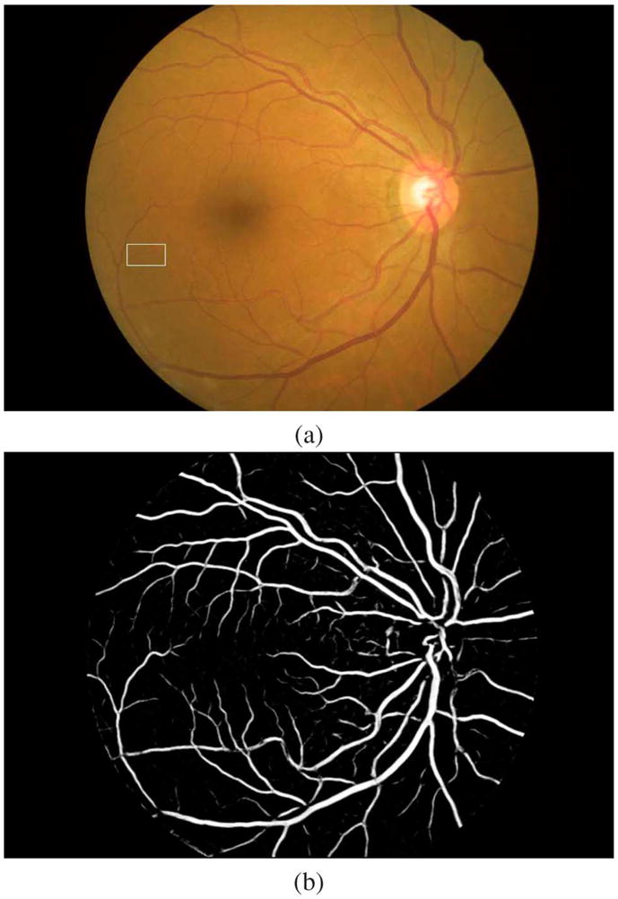
An example vesselness image calculated using [9]. (a) The color fundus image. The white rectangular is enlarged and used for illustration in Fig. 2. (b) The corresponding vesselness image.
From this vessel centerline image, the bifurcation points and crossing points are excluded, because these points need special treatment. A bifurcation point is defined as a centerline pixel with three eight-connected neighbors and a crossing point is defined as a centerline pixel with four or more eight-connected neighbors. Hence, the vessel centerline image is scanned first to get the centerline pixels that have three or more neighbors. By deleting the bifurcation points and crossing points, the vessel trees are cut into vessel segments. From these vessel segments, the end points which have only one neighbor pixel are found by scanning the image again. Starting from one end point, we then trace the vessel segment until the other end point is reached. In this way, we trace all the vessel segments on the image and label each of them.
C. Graph-Based Vessel Boundary Segmentation
For each labeled vessel segment, the growing direction for every centerline pixel is calculated. We use n adjacent center-line pixels on both sides of the target centerline pixel and apply principal component analysis on the resulting vessel segment [19]. The value of n is a parameter of the image size, which is approximately 0.005 times the first dimension of the image size. So if the first dimension of an image is 600 pixels, the value of n would be three pixels, resulting in a total vessel segment length of seven pixels. The minimum value of n is two. The first principal component corresponds to the growing direction of the pixel. An end point that does not have enough neighboring centerline pixels to define the vessel growing direction is determined to have the direction of the nearest centerline pixel that has a definition of a vessel growing direction.
For the vessel growing direction, a counter-clockwise 90° is regarded as the normal direction for this point. Using the center-line pixels as the base nodes, profiles on the positive direction of the normals are built as one slice and profiles on the negative direction are built as another slice, as shown in Fig. 2. The node step was 0.5 pixels. We used the “multicolumn model” proposed by Li et al. [7].
Fig. 2.

An illustration of how to luxate the vessel normal profiles into a graph. (a) A small segment of vessel extracted from Fig. 1. (b) The vessel probability image of (a). (c) The vessel centerline image of (a). (d) The vessel growing directions are calculated and node normal profile perpendicular to the vessel growing direction are constructed. (e) Red normal profiles in (d) are used to build the red graph slice and the green normal profiles in (d) are used to build the green graph slice. The black nodes represent base nodes, corresponding to the black centerline pixels in (d). Consequently, the red slice represents one boundary in (d) and the green slice represents the other boundary in (d). Smoothness constraints (controlled by the arcs between adjacent columns) are applied differently to control the boundary smoothness within one boundary and between the two boundaries.
Along each normal profile Col(x, y) every node V(x, y, z) (z > 0) has a directed arc to the node V(x, y, z − 1). Along the x-direction, meaning along the same boundary, for each node, a directed arc is constructed from to V(x, y, z) ∈ Col(x, y) to V(x + 1, y, max(0, z − Δx)) ∈ Col(x + 1, y). Similarly, arcs from V(x, y, z) ∈ Col(x, y) to V(x − 1, y, max(0, z − Δx)) ∈ Col(x − 1, y, z) is constructed. Δx is the maximum difference allowed between two adjacent normal profiles within one boundary. Along the y-direction, meaning between the two slices, arcs from V(x, y, z) ∈ Col(x, y) to V(x, y + 1, max(0, z − Δy)) ∈ Col(x, y + 1, z) and arcs from V(x, y, z) ∈ Col(x, y) to V(x, y − 1, max(0, z − Δy)) ∈ Col(x y − 1, z) is constructed. Δy is the maximum difference allowed between two corresponding normal profiles between the two boundaries. The base nodes are all connected [7]. A surface is regarded feasible if it satisfies the smoothness constraint defined by Δx and Δy. An optimal surface is defined as the surface with the minimum cost among all feasible surfaces defined in the 3-D volume.
D. Cost Function
The cost image is generated from the orientation sensitive 1-D first-order derivative of Gaussian of the green channel. During development, 2-D Gaussian derivatives, differences of Gaussian, and Canny edge filters were also tested for enhancement, but were discarded because they were not robust enough across the wide variety of vessel widths. The green channel of the color image usually shows the highest contrast between the blood vessels and background [16].
In order to find the gradient of vessels specified at different locations with different orientations, a discrete convolution with the 1-D derivative of Gaussian is applied along the direction perpendicular to the vessel growing direction (as shown in Fig. 3). The derivative of Gaussian kernel is shown in
Fig. 3.

Gradient image. (a) Part of a green channel image. (b) The corresponding orientation sensitive gradient image.
| (1) |
where σ is the only parameter in the first order derivative of Gaussian. Fig. 3 is an example. Fig. 3(a) shows an enlarged part of the green channel image. Fig. 3(b) shows the orientation sensitive 1-D derivative of Gaussian result.
E. Graph Search and Boundary Determination
The value of Δx is set to one to maintain the smoothness within one boundary and Δy is set to two so that a difference is allowed between widths from the centerline to the left edge and from the centerline to the right edge, in case the centerline is not exactly at the center of the two edges. After the node-weighted directed graph is constructed, the optimal surface is determined [7]. To determine the vessel width, the coordinate difference between the two corresponding nodes on the optimal surface from the two slices is calculated. To show the boundary on the image, the nearest integer coordinate of every node on the optimal surface is calculated and shown on the image.
F. Experimental Methods
1) Validation on Human Expert Derived Vessel Widths
The REVIEW database were used to validate the correctness of the algorithm. Each profile in the REVIEW database consists of 15 numbers: series number, image number, segment number and four data for each of the three observers. The three observers are denoted as O1, O2 and O3. For each observer, there are four measurements for two points on each edge (x1, y1, x2 and y2). The vessel centerline is defined as [(x1 + x2)/(2), (y1 + y2)/(2)] and the vessel width as for each observer (http://ReviewDB.lincoln.ac.uk). A reference standard, denoted by RS, is then created by averaging the manual results of the three observers.
We determine the vessel centerlines as explained in Section III-B above, and mapped to the centerlines in the RS, so that only those vessel centerline pixels were analyzed that also occurred in the RS. Otherwise the centerline pixel is labeled as absent.
We also compared our method with the results of the methods provided in Al-Diri’s paper [13], where 1DG and 2DG mean 1-D Gaussian model-fitting and 2-D Gaussian model-fitting [20], [21], respectively. However, standard deviations of vessel width differences are not provided in that paper.
2) Determination the Relationship Between Vessel Width and Distance From the Optic Disc Center
To determine this relationship on the dataset of 600 registered fundus images we proceeded as explained in Section III-E to obtain the vessel widths of all vessels. Circular regions of interest one pixel wide were centered on the optic disc center. The average width of all vessels in each region of interest (i.e., both arteries and veins) was then plotted in a graph, as well as the 95% confidence interval (CI) of the average width. Centerline pixels with a distance larger than 450 pixels from the disc were too close to the edge of the image—less than 2.1% of all centerline pixels—and were eliminated from further analysis.
IV. Results
A. Validation on Human Expert Derived Vessel Widths
An example of the quality of the obtained vessel boundary detection is shown in Fig. 4. It shows a good performance on even the smallest vessels, which have low contrast.
Fig. 4.

Sample images showing the result of vessel boundary detection. (a) One image from the CLRIS database. Image size is 2160 × 1440, σ = 0. (b) A enlarged part of image (a).
The proposed method were compared to the other known algorithms in Tables I–IV. The first three rows are the manual results from the observers. Row 4–8 show the results of the other algorithms. The last row shows the result of the proposed method. The first column is the success rate. It is worth noticing that the definition of success rate is different in our method and in Al-Diri’s paper. In their paper, a point that has a meaningful measurement (e.g., a measurement that converges) was assigned “success measurement” [13]. In contrast, we counted every centerline pixel that had corresponding ground truth profiles as a “success measurement,” irrespective of our estimate of the width. Therefore all measurements with a corresponding ground truth profile were included even if the measurements did not result in a meaningful estimation. The columns 2–3 are the mean and standard deviation of all measurements labeled as “success measurement.” Column 4–5 are the signed mean and standard deviation of the point-by-point differences.
TABLE I.
Vessel Width Measurement Accuracy OF HRIS (Success Rate IN Percentage, Mean μ, AND Standard Deviation σ IN Pixel)
| Method Name | Success Rate % | Measurement | Difference | ||
|---|---|---|---|---|---|
| μ | σ | μ | σ | ||
| Observer 1 (O1) | 100 | 4.12 | 1.25 | −0.23 | 0.288 |
| Observer 2 (O2) | 100 | 4.35 | 1.35 | 0.002 | 0.256 |
| Observer 3 (O3) | 100 | 4.58 | 1.26 | 0.23 | 0.285 |
| Gregson’s Algorithm | 100 | 7.64 | - | 3.29 | 2.841 |
| Half-height full-width (HHFW) | 88.3 | 4.97 | - | 0.62 | 0.926 |
| 1-D Gaussian Model-fitting | 99.6 | 3.81 | - | −0.54 | 4.137 |
| 2-D Gaussian Model-fitting | 98.9 | 4.18 | - | −0.17 | 6.019 |
| Extraction of Segment Profiles (ESP) | 99.7 | 4.63 | - | 0.28 | 0.42 |
| Proposed Method | 100 | 4.56 | 1.30 | 0.21 | 0.567 |
TABLE IV.
Vessel Width Measurement Accuracy OF KPIS (Success Rate IN Percentage, Mean μ, AND Standard Deviation σ IN Pixel)
| Method Name | Success Rate % | Measurement | Difference | ||
|---|---|---|---|---|---|
| μ | σ | μ | σ | ||
| Observer 1 (O1) | 100 | 7.97 | 0.47 | 0.45 | 0.234 |
| Observer 2 (O2) | 100 | 7.60 | 0.42 | 0.08 | 0.213 |
| Observer 3 (O3) | 100 | 7.00 | 0.52 | −0.52 | 0.233 |
| Gregson’s Algorithm | 100 | 7.29 | - | −0.23 | 0.602 |
| Half-height full-width (HHFW) | 96.3 | 6.47 | - | −1.05 | 0.389 |
| 1-D Gaussian Model-fitting | 100 | 4.95 | - | −2.57 | 0.399 |
| 2-D Gaussian Model-fitting | 100 | 5.87 | - | −1.65 | 0.337 |
| Extraction of Segment Profiles (ESP) | 100 | 6.56 | - | −0.96 | 0.328 |
| Proposed Method | 99.4 | 6.38 | 0.59 | −1.14 | 0.67 |
Among the four datasets, the HRIS dataset has the highest image resolution (3584 × 2438 pixels). The performance of the vessel width detection is comparable to the observers. The CLRIS dataset images have a resolution of 2160 × 1440 pixels. The mean vessel width and the point-by-point difference mean are very close to the observers’ performance. But the point-by-point difference standard deviation is high. The VDIS dataset has a resolution of 1360 × 1024 pixels. The mean vessel width is 0.53 pixels smaller than the ground truth. The KPIS dataset has the smallest image resolution, 288 × 119 pixels and 170 × 92 pixels.
Our testing indicates that fundus images with a higher resolution can be measured more accurately with a larger σ. The final choice of σ is σ = 7 for HRIS dataset, σ = 4 for CLRIS and VDIS, σ = 1 for KPIS.
Fig. 5 shows the correlation of predicted vessel width and the mean of the observers’ measurements for HRIS. The regression line shows the prediction tends to give a smaller measurement for vessels with fine vessels while a larger measurement for large vessels, compared to the observers’ measurements.
Fig. 5.
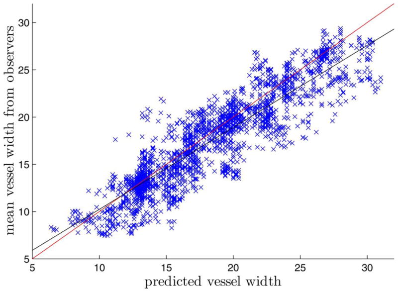
Correlation of predicted vessel width and the mean of the observers’ measurements for HRIS. Each point represent one profile. The red line is the y = x line. The black line is the regression line (y = 0.87x + 1.56).
B. Determining the Relationship Between Vessel Width and Distance From the Optic Disc Center
The relationship between vessel width and distance from the optic disc center is shown in Fig. 6. A total of 2 936 749 centerline pixels were extracted from the 600 images. If we do not consider the pixels near the center of optic disc, where the blood vessels show a very complicated structure, the average vessel width shows a monotonic decrease from a distance of 20 pixels to 450 pixels, with a sudden slope change at a distance of 300 pixels to the optic disc. For vessels near the optic disc border, the average vessel width is about 5.0 pixels (approximately 75 μm) while the vessels that have a distance of 450 pixels to the optic disc have an average vessel width of 3.5 pixels (approximately 52.5 μm).
Fig. 6.
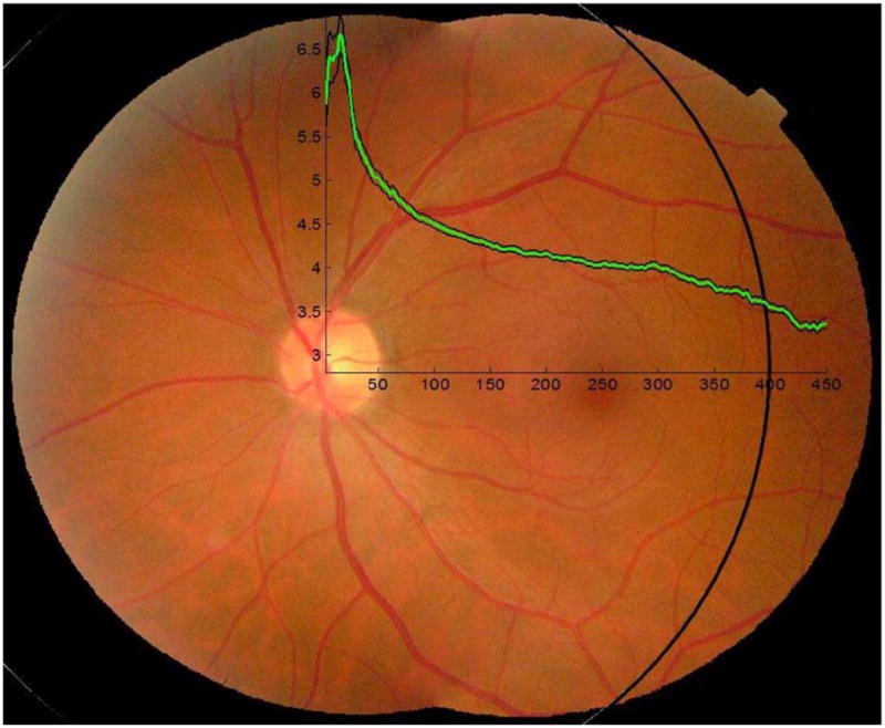
A relationship between vessel width and distance to optic disc. The black circle marks a 400 pixels to the optic disc center. The vessel width analysis starts from the optic disc center and ends at a distance of 450 pixels (the x-axis). The y-axis shows the vessel width in pixels. The green line is the average vessel width. The black lines are the 95% confidence interval lines. Image resolution is about 800 × 700 pixels. Scale parameter σ = 4 pixels was used.
V. Discussion
We introduced a novel method to find the retinal blood vessel boundaries using a graph-based approach. The results of our evaluation show that the blood vessel boundaries are accurate, and our method outperforms the current state-of-the-art algorithm on two datasets of standard retinal image resolution, while it under-performs on lower resolution retinal images [13], as further discussed in Section V-A. Our method allows us to find the retinal vessel boundaries of even small vessels on standard posterior pole images as used in diabetic retinopathy screening programs around the world [22]. Though the performance on the HRIS and CLRIS was close to the human experts reference standard, it tends to be biased towards showing a smaller measurement, for smaller vessels. The most likely explanation is that the vessel width measurement is done with a fixed scale parameter, while the optimal measurement of vessels in different scales need different scale parameters. A multiscale cost function is under study to solve this problem.
Alternatively, vessel width can be measured directly from the vesselness map. In a preliminary experiment, we thresholded the vesselness image, generating a binary vessel segmentation. A fixed threshold of 190 was used. Width were then measured on this binary vessel map, resulting, on the HRIS dataset, in average vessel width of 6.5 pixels, with a standard deviation of 32.52 pixels. Therefore, the vesselness map itself gave a poor estimation of the mean of vessel width, with a standard deviation about 30 times higher than other methods, which makes this approach unfeasible.
A. Width Measurement on Images of Different Resolution
The proposed method showed a consistently underestimated vessels in (comparing with RS) low resolution images, especially for the KPIS dataset, where the point-by-point difference is −1.14 pixels. But we also noticed that all other algorithms in Table IV also underestimated the width. Fig. 7 illustrates the RS and the algorithmic estimates on vessel segments from a high resolution image and a low resolution image. This is a cross-sectional view of vessel intensity with regard to the distance to the centerline. The black line is the average intensity of all normal profile nodes with the same distance to the centerline in the vessel segments. The red star is the average vessel width across the whole vessel segment marked by observers. The green star is the average vessel width across the whole vessel segment measured by proposed method. The HRIS image has a resolution of 3584 × 2438 pixels. The vessel segment has a mean vessel width of about 26 pixels and the edge crosses about ten pixels. The KPIS image has a resolution of 288 × 119 pixels. The vessel segment has a mean vessel width of about seven pixels and the edge crosses about three pixels. This figure suggests the underlying standards for width measurement of vessels in different scales are different. On the HRIS vessel segment, both the RS and the proposed method found the location with the maximum gradient as the vessel edge. However, on the KPIS vessel segment, the RS and the proposed method give different measurements. The observers on average give a larger measurement on those low resolution vessels.
Fig. 7.

Vessel width measurement on vessel segments with different resolutions. (a) One test vessel segment from HRIS. The length of the vessel segment is 173 pixels. (b) One Test vessel segment from KPIS. The length of the vessel segment is 226 pixels. (c) The vessel width measurement result of (a). If the detected edge is not at an integer location, the nearest integer coordinate is shown. (d) The vessel width measurement result of (b). If the detected edge is not at an integer location, the nearest integer coordinate is shown. (e) The cross-sectional view of vessel intensity with regard to the distance to the centerline for (a). The black curve is the average of 173 normal profiles in the vessel segment. Intensities at noninteger locations are linearly interpolated. The red star is the average vessel width across the whole vessel segment marked by observers. The green star is the average vessel width across the whole vessel segment measured by proposed method. The two boundaries are flipped and shown in one figure. (f) The cross-sectional view of vessel intensity with regard to the distance to the centerline for (b). The black curve is the average of 226 normal profiles in the vessel segment. Intensities at noninteger locations are linearly interpolated. The red star is the average vessel width across the whole vessel segment marked by observers. The green star is the average vessel width across the whole vessel segment measured by proposed method. The two boundaries are flipped and shown in one figure.
B. Vessel Width and Distance to the Optic Disc
Our results show that the relationship between vessel width with distance and the optic disc center is inverse and monotonous. Using this method, we were able to reliably determine the relationship between the average retinal vessel diameter and the distance from the optic disc from 600 patients with diabetes. Except for the vessel pixels near the center of the optic disc (about 20 pixels), the blood vessel width shows a monotonic decrease considering the distance from the optic disc to the center. This is most likely caused by branching—if we assume the blood vessel volume to be unchanged. If the number of blood vessels is kept constant, the higher the branch frequency with increasing distance to the optic disc, the larger the slope of the width decrease. At a distance of around 300 pixels, there is a slight slope change in average vessel width, most likely caused by the fact that this is where the image centered on the optic disc ends and transitions to the fovea centered image that is registered to it in our dataset.
Though our method has been tested on retinal images only, it may be equally effective on other 2-D blood vessel projections such as cardiac and brain angiograms.
C. Computational Performance
The proposed method has a high computational performance. For a retinal image of size 2160 × 1440 pixels, vesselness map creation takes about 110 s, and this is an operation
 (n), where n is the number of pixels. The image skeletonization and small region removal takes about 120 s, and this is also an operation
(n). The total number of centerline pixels is around 20 000 pixels (or 0.0064n) and the total number of vessel segments is 160. Consequently the average length of the graph is around 125 pixels. The average size of the graph would be slice number × height of graph × length of graph, which is 45 000 (or 0.0145n) in this case. It takes around 9 s to build all the graphs in the image. The method we used to solve the max-flow problem is a pseudoflow algorithm. The running time is
(n3) [23]. It takes about 41 s to solve all the graphs in the example image.
(n), where n is the number of pixels. The image skeletonization and small region removal takes about 120 s, and this is also an operation
(n). The total number of centerline pixels is around 20 000 pixels (or 0.0064n) and the total number of vessel segments is 160. Consequently the average length of the graph is around 125 pixels. The average size of the graph would be slice number × height of graph × length of graph, which is 45 000 (or 0.0145n) in this case. It takes around 9 s to build all the graphs in the image. The method we used to solve the max-flow problem is a pseudoflow algorithm. The running time is
(n3) [23]. It takes about 41 s to solve all the graphs in the example image.
D. Limitations
Our approach has some limitations. It relies largely on the initial segmentation, the vesselness image. False positives or disconnected vessels may result in incorrect vessel boundary detection and vessel diameter measurements. A low threshold value and spur pruning is one possible way to reduce the problem. But the trade-off is the loss of some fine vessel information.
The crossing points and branching points are currently not treated separately, because the vessel growing direction, and consequently the vessel normal direction, at those points are not well defined. This does not have a significant influence on the vessel diameter measurements. However, the generation of the continuous vessel tree will require the vessels be connected at the crossing and branching points. A possible method to solve the direction problem at the crossing points and branching points is the distance transform of the vessel centerline image. For the crossing points, branching points and centerline pixels near them, the direction with the maximum gradient can be considered as the normal profile direction. Another solution is detecting and dealing with the crossing and branching points explicitly.
VI. Conclusion
We proposed a novel method for retinal vessel boundary detection based on graph search and validated it on a publicly available dataset of expert annotated vessel widths. An important advantage is that this method detects both boundaries simultaneously, and is therefore more robust than methods which detect the boundaries one at a time. The simultaneous detection of both borders makes the accurate detection possible even if one boundary is of low contrast or blurred. Overall, the method is robust as the only algorithmic parameter is σ in the cost function, and the final measurement is insensitive to the choice of σ.
In summary, we have developed and validated a fast and automated method for measurement of retinal blood vessel width. We expect that such methods have potential for a novel quantitative approach to early detection of retinal and cardiovascular disease.
TABLE II.
Vessel Width Measurement Accuracy OF CLRIS (Success Rate IN Percentage, Mean μ, AND Standard Deviation σ IN Pixel)
| Method Name | Success Rate % | Measurement | Difference | ||
|---|---|---|---|---|---|
| μ | σ | μ | σ | ||
| Observer 1 (O1) | 100 | 13.19 | 4.01 | −0.61 | 0.566 |
| Observer 2 (O2) | 100 | 13.69 | 4.22 | −0.11 | 0.698 |
| Observer 3 (O3) | 100 | 14.52 | 4.26 | 0.72 | 0.566 |
| Gregson’s Algorithm | 100 | 12.8 | - | −1.0 | 2.841 |
| Half-height full-width (HHFW) | 0 | - | - | - | - |
| 1-D Gaussian Model-fitting | 98.6 | 6.3 | - | −7.5 | 4.137 |
| 2-D Gaussian Model-fitting | 26.7 | 7.0 | - | −6.8 | 6.019 |
| Extraction of Segment Profiles (ESP) | 93.0 | 15.7 | - | −1.90 | 1.469 |
| Proposed Method | 94.1 | 14.05 | 4.47 | 0.08 | 1.78 |
TABLE III.
Vessel Width Measurement Accuracy OF VDIS (Success Rate IN Percentage, Mean μ, AND Standard Deviation σ IN Pixel)
| Method Name | Success Rate % | Measurement | Difference | ||
|---|---|---|---|---|---|
| μ | σ | μ | σ | ||
| Observer 1 (O1) | 100 | 8.50 | 2.54 | −0.35 | 0.543 |
| Observer 2 (O2) | 100 | 8.91 | 2.69 | 0.06 | 0.621 |
| Observer 3 (O3) | 100 | 9.15 | 2.67 | 0.30 | 0.669 |
| Gregson’s Algorithm | 100 | 10.07 | - | 1.22 | 1.494 |
| Half-height full-width (HHFW) | 78.4 | 7.94 | - | −0.91 | 0.879 |
| 1-D Gaussian Model-fitting | 99.9 | 5.78 | - | −3.07 | 2.110 |
| 2-D Gaussian Model-fitting | 77.2 | 6.59 | - | −2.26 | 1.328 |
| Extraction of Segment Profiles (ESP) | 99.6 | 8.80 | - | −0.05 | 0.766 |
| Proposed Method | 96.0 | 8.35 | 3.00 | −0.53 | 1.43 |
Acknowledgments
This work was supported in part by the National Eye Institute (R01 EY017066), in part by Research to Prevent Blindness, NY, and in part by the Department for Veterans Affairs.
Contributor Information
Xiayu Xu, Department of Biomedical Engineering, University of Iowa, Iowa City, IA 52242 USA.
Meindert Niemeijer, Departments of Ophthalmology and Visual Sciences and Electrical and Computer Engineering, University of Iowa, Iowa City, IA 52242 USA, and also with the Veteran’s Administration Medical Center, Iowa City, IA 52242 USA.
Qi Song, Department of Electrical and Computer Engineering, University of Iowa, Iowa City, IA 52242 USA.
Milan Sonka, Departments of Ophthalmology and Visual Sciences and Electrical and Computer Engineering, University of Iowa, Iowa City, IA 52242 USA, and also with the Veteran’s Administration Medical Center, Iowa City, IA 52242 USA.
Mona K. Garvin, Department of Electrical and Computer Engineering, University of Iowa, Iowa City, IA 52242 USA.
Joseph M. Reinhardt, Department of Biomedical Engineering, University of Iowa, Iowa City, IA 52242 USA.
Michael D. Abràmoff, Departments of Ophthalmology and Visual Sciences, Biomedical Engineering, and Electrical and Computer Engineering, University of Iowa, Iowa City, IA 52242 USA, and also with the Veteran’s Administration Medical Center, Iowa City, IA 52242 USA.
References
- 1.Klein R, Klein B, Moss S. The relation of systemic hypertension to changes in the retinal vasculature: The beaver dam eye study. Trans Amer Ophthalmological Soc. 1997;95:329–350. [PMC free article] [PubMed] [Google Scholar]
- 2.Klein R, Klein B, Moss S, Wang Q. Hypertension and retinopathy, arteriolar narrowing and arteriovenous ricking in a population. Arch Ophthalmol. 1994;112(1):92–98. doi: 10.1001/archopht.1994.01090130102026. [DOI] [PubMed] [Google Scholar]
- 3.Hubbard L, Brothers R, King W, Clegg L, Klein R, Cooper L, Sharrett A, Davis M, Cai J. Methods for evaluation of retinal microvascular abnormalities associated with hypertension/sclerosis in the atherosclerosis risk in communities study. Opthalmology. 1999 Dec 1;106(12):2269–2280. doi: 10.1016/s0161-6420(99)90525-0. [DOI] [PubMed] [Google Scholar]
- 4.Niemeijer M, van Ginneken B, Abramoff MD. Automatic determination of the artery vein ratio in retinal images. SPIE Med Imag. 2010;7624 [Google Scholar]
- 5.Fairfield J. Toboggan contrast enhancement for contrast segmentation. Proc Int Conf Pattern Recognit. 1990:712–716. [Google Scholar]
- 6.Hu Z, Abramoff MD, Kwon YH, Lee K, Garvin M. Automated segmentation of neural canal opening and optic cup 3D spectral optical coherence tomography volumes of the optic nerve head. Invest Ophthalmol Vis Sci. 2010:5708–5717. doi: 10.1167/iovs.09-4838. [DOI] [PMC free article] [PubMed] [Google Scholar]
- 7.Li K, Wu X, Chen DZ, Sonka M. Optimal surface segmentation in volumetric images—A graph-theoretic approach. IEEE Trans Pattern Anal Mach Intell. 2006 Jan;28(1):119–134. doi: 10.1109/TPAMI.2006.19. [DOI] [PMC free article] [PubMed] [Google Scholar]
- 8.Joshi V, Reinhardt JM, Abramoff MD. Automated measurement of retinal blood vessel tortuosity. SPIE Med Imag. 2010;7624 [Google Scholar]
- 9.Niemeijer M, Staal J, van Ginneken B, Loog M, Abramoff M. Comparative study of retinal vessel segmentation methods on a new publicly available database. SPIE Med Imag. 2004;5370:648–656. [Google Scholar]
- 10.Staal J, Abrámoff MD, Niemeijer M, Viergever MA, van Ginneken B. Ridge-based vessel segmentation in color images of the retina. IEEE Trans Med Imag. 2004 Apr;23(4):501–509. doi: 10.1109/TMI.2004.825627. [DOI] [PubMed] [Google Scholar]
- 11.Gang L, Chutatape O, Krishnan SM. Detection and measurement of retinal vessels in fundus images using amplitude modified second-order gaussian filter. IEEE Trans Biomed Eng. 2002 Feb;49(2):168–172. doi: 10.1109/10.979356. [DOI] [PubMed] [Google Scholar]
- 12.Lalonde M, Gagnon L, Boucher M-C. Non-recursive paired tracking for vessel extraction from retinal images. Proc Conf Vis Interface. 2000:61–68. [Google Scholar]
- 13.Al-Diri B, Hunter A, Steel D. An active contour model for segmenting and measuring retinal vessels. IEEE Trans Biomed Eng. 2009 Sep;29(9):1488–1497. doi: 10.1109/TMI.2009.2017941. [DOI] [PubMed] [Google Scholar]
- 14.Brinchmann-Hansen O, Heier H. Theoretical relations between light streak characteristics and optical properties of retinal vessels. Acta Ophthalmologica, Suppl. 1986;179:33–37. [Google Scholar]
- 15.Gregson P, Shen Z, Scott R, Kozousek V. Automated grading of venous beading. Comput Biomed Res. 1995 Aug;28(4):291–304. doi: 10.1006/cbmr.1995.1020. [DOI] [PubMed] [Google Scholar]
- 16.Lee S, Abramoff MD, Reinhardt JM. Retinal atlas statistics from color fundus images. SPIE Med Imag. 2010;7623:762310. [Google Scholar]
- 17.Abramoff MD, Niemeijer M. The automatic detection of the optic disc location in retinal images using optic disc location regression. IEEE EMBS Conf. 2006:4432–4435. doi: 10.1109/IEMBS.2006.259622. [DOI] [PMC free article] [PubMed] [Google Scholar]
- 18.Sonka M, Hlavac V, Boyle R. Image Processing, Analysis, and Machine Vision. New York: PWS; 1998. [Google Scholar]
- 19.Shlens J. A tutorial on principal component analysis 2005 [Online] Available: http://www.snl.salk.edu/shlens/pub/notes/pca.pdf.
- 20.Lowell J, Hunter A, Stell D, Basu A, Ryder R, Kennedy R. Measurement of retinal vessel widths from fundus images based on 2-D modeling. IEEE Trans Med Imag. 2004 Oct;23(10):1196–1204. doi: 10.1109/TMI.2004.830524. [DOI] [PubMed] [Google Scholar]
- 21.Zhou L, Rzezotarski M, Singerman L, Chokreff J. The detection and quantification of retinopathy using digital angiograms. IEEE Trans Med Imag. 1994 Dec;13(4):619–626. doi: 10.1109/42.363106. [DOI] [PubMed] [Google Scholar]
- 22.Abramoff MD, Suttorp-Schulten MS. Automatic detection of red lesions in digital color fundus photographs. Telemedicine E-Health. 2005;11(6):668–674. doi: 10.1109/TMI.2005.843738. [DOI] [PubMed] [Google Scholar]
- 23.Chandran BG, Hochbaum DS. A computational study of the pseudoflow and push-relabel algorithms for the maximum flow problem. RAIRO Oper Res. 2009;57(2):358–376. [Google Scholar]