Regularized Image Reconstruction Algorithms for Dual-Isotope Myocardial Perfusion SPECT (MPS) Imaging Using a Cross-Tracer Prior

Abstract

In simultaneous dual-isotope myocardial perfusion SPECT (MPS) imaging, data are simultaneously acquired to determine the distributions of two radioactive isotopes. The goal of this work was to develop penalized maximum likelihood (PML) algorithms for a novel cross-tracer prior that exploits the fact that the two images reconstructed from simultaneous dual-isotope MPS projection data are perfectly registered in space. We first formulated the simultaneous dual-isotope MPS reconstruction problem as a joint estimation problem. A cross-tracer prior that couples voxel values on both images was then proposed. We developed an iterative algorithm to reconstruct the MPS images that converges to the maximum a posteriori solution for this prior based on separable surrogate functions. To accelerate the convergence, we developed a fast algorithm for the cross-tracer prior based on the complete data OS-EM (COSEM) framework. The proposed algorithm was compared qualitatively and quantitatively to a single-tracer version of the prior that did not include the cross-tracer term. Quantitative evaluations included comparisons of mean and standard deviation images as well as assessment of image fidelity using the mean square error. We also evaluated the cross tracer prior using a three-class observer study with respect to the three-class MPS diagnostic task, i.e., classifying patients as having either no defect, reversible defect, or fixed defects. For this study, a comparison with conventional ordered subsets-expectation maximization (OS-EM) reconstruction with postfiltering was performed. The comparisons to the single-tracer prior demonstrated similar resolution for areas of the image with large intensity changes and reduced noise in uniform regions. The cross-tracer prior was also superior to the single-tracer version in terms of restoring image fidelity. Results of the three-class observer study showed that the proposed cross-tracer prior and the convergent algorithms improved the image quality of dual-isotope MPS images compared to OS-EM.

I. Introduction

Penalized maximum likelihood (PML) image reconstruction methods have been used extensively to address the ill-posed nature of emission image reconstruction. In particular, various penalty functions have been developed to penalize the maximum likelihood (ML) solution of the emission reconstruction problem to lower the noise in nuclear medicine images. These penalty functions, or priors, penalize images that exhibit large differences between nearby voxels.

In some nuclear medicine imaging protocols, multiple images are obtained for the same patient characterizing different functional or anatomical properties. For example, in simultaneous dual-isotope myocardial perfusion SPECT (MPS) imaging, two images are acquired simultaneously, representing the distributions of two radioactive isotopes. Due to the simultaneous acquisition, the two images are perfectly registered in time and space. We hypothesize that common information in the registered data can be used to improve the overall image quality. The goal of this study was to develop a cross-tracer prior that uses this common information and penalizes both images simultaneously, to develop converging PML algorithms for the cross-tracer prior, and to compare the new reconstruction method, using task-based performance measures, to a conventional separate reconstruction technique.

A. Simultaneous Dual-Isotope Myocardial Perfusion SPECT

In a simultaneous dual-isotope MPS imaging protocol, radiopharmaceuticals labeled with two isotopes, ^99mTc and ²⁰¹Tl, are simultaneously present in the patient body. Projection data are acquired and two images are reconstructed, thus simultaneously characterizing the stress and rest states of myocardial perfusion. Since the projection data are acquired simultaneously, the two reconstructed images are thus perfectly registered. The diagnosis of coronary artery disease (CAD) using MPS considers defect presence in both images and classifies patients as being normal, having reversible ischemia, or fixed perfusion defects, as shown in Table I.

TABLE I.

Three Classes in Simultaneous Dual-Isotope MPS Imaging

	Class 1	Class 3	Class 2
	Normal	Reversible defect	Fixed defect
Tc-99m (stress)	No*	Yes**	Yes
Tl-201 (rest)	No	No	Yes

^*No denotes perfusion defect absence

^**Yes denotes perfusion defect presence

One limiting problem in simultaneous dual isotope imaging is crosstalk contamination between the projection data from the two isotopes. We have previously developed methods to model [1], [2] and compensate for [3] this contamination using iterative reconstruction algorithms. We have also shown the efficacy of these methods in improving image quality compared to the case of no crosstalk compensation. While crosstalk compensation was effective, task performance was still degraded compared to separate acquisition. We believe that a major reason for this is the increase in noise in the compensated dual isotope image compared to the separate acquisition. Specifically, the compensation method can, at best, estimate only the mean of the crosstalk, leaving behind the noise from the crosstalk. As an example, assume that a uniform background is added to projections, which are thus corrupted by Poisson noise. Subtracting the background would remove the bias, but not the noise from the crosstalk. The goal of this work is to exploit the perfect registration of the simultaneous dual isotope images to reduce the impact of this noise on task performance.

B. Motivation for the Cross-Tracer Prior

To motivate the hypothesis that the perfectly registered images can be used to improve image quality, we performed an experiment using data from [4]. In this study, we evaluated the image quality of dual-isotope MPS imaging using a large simulated image ensemble, reconstructed with OS-EM algorithms with attenuation, scatter and detector response compensation. The image ensemble is described in more detail in Section III. We used a two-class observer study to assess defect detectability using either the image of the isotope itself, or with the addition of data from the other isotope. We investigated two cases. First we investigated defect detection performance in the ^99mTc image with and without access to the ²⁰¹Tl image. In this case, the ²⁰¹Tl image was defect free regardless of the state of the ^99mTc image. Thus, detecting the defect in the ^99mTc data distinguished between normal and reversible lesions. In the second case, we investigated defect detection performance in the ²⁰¹Tl image with and without access to the ^99mTc image. For this case, the image had a defect present in all cases, and detecting the defect in the ²⁰¹Tl image thus distinguished between patients with fixed or reversible defects.

Table II shows the AUC values obtained using reconstructed images from both separate and simultaneous acquisitions. The left half of Table II shows the AUC values for classifying normal patients versus patients with reversible defects using the ^99mTc image alone or using both images. Similarly, the right half of Table II shows the AUC values for classifying patients with fixed versus reversible defects using the ²⁰¹Tl image only or both images. In both cases, using both the ^99mTc and ²⁰¹Tl images resulted in a higher AUC value than using only one of the images. These results indicate that, despite the fact that the image from one of the isotopes did not explicitly contain information about whether there was a defect present in the other image, access to that image improved defect detection performance. This observation suggests that successfully using this information during the reconstruction might improve the overall image quality, i.e., the ability to correctly classify into the three diagnostic classes.

TABLE II.

Comparison of Two-Class AUC Values Using Single and Dual Isotope Data

	Normal vs. Reversible		Fixed vs. Reversible
	Separate	Simultaneous	Separate	Simultaneous
Tc data only	0.888	0.886	0.888	0.870	Tl data only
Tc+Tl data	0.946	0.937	0.917	0.890	Tc+Tl data

C. Application of the Penalized Maximum Likelihood (PML) Algorithms

As shown above, incorporating the information provided by the other isotope may improve the image quality, and simultaneous acquisition provides a convenient means to enable this since the acquired data are perfectly registered. The goal of this work was thus to develop fast and convergent PML algorithms that integrate the information on images from both isotopes. Many challenges exist in accomplishing this goal.

The first challenge was development of a prior that couples the information on both stress and rest images. One way of achieving this would be to use 4D maximum a posteriori (MAP) reconstruction algorithms. In these algorithms, a time domain clique is employed and a time domain smoothing term is incorporated into the prior to penalize differences in corresponding voxel values on images from different time frames. This is possible because it is assumed that the voxel values are continuous in the time domain. In dual-isotope MPS imaging, however, the voxel values are not necessarily related in the two images. Instead, general anatomical features, such as anatomical boundaries, are common. We used this, as well as constraints on the prior form needed to develop a convergent algorithm, and designed a cross-tracer prior that will be described in detail below. Based on this cross-tracer prior, the dual-isotope MPS reconstruction algorithm was formulated as a joint estimation problem.

A second challenge lies in the development of a convergent PML algorithm for the proposed cross-tracer prior. Converging PML algorithms have been investigated for different types of priors, and many optimization techniques have been used in the literature [5]–[8]. We chose to use optimization transfer methods [9], which replace the original cost function at each step with a surrogate function. The surrogate function is selected so that it is easier to optimize and often a closed-form solution update equation exists. In addition, compared to other approaches, reduced computation time is possible for a carefully chosen surrogate function. Thus, the essence of the second challenge is to carefully choose surrogate functions. De Pierro proposed certain surrogate functions for MAP algorithms based on the concavity of the log-likelihood function and the convexity of certain penalty functions, but derived closed form solutions only for quadratic priors [7]. Based on De Pierro’s approach, Chang demonstrated that closed-form solutions are possible for a group of nonquadratic Gibbs priors [10]. In this work, we adopted Chang’s approach to derive a separable surrogate function for the proposed cross-tracer prior.

The third challenge is to accelerate the algorithm using ordered subsets while still maintaining the convergence of the algorithm. A fast converging MAP algorithm, row-action maximum-likelihood algorithm (RAMLA), was proposed by Browne et al., based on the row-action Algebraic Reconstruction Technique (ART) algorithm, by introducing a subset-independent diminishing step size [11]. Based on Browne’s work, Ahn et al. proposed a modified block sequential regularized expectation maximization (BSREM) algorithm, which allows more convenient selection of the relaxation parameters [8]. However, the relaxation scheme selection must be performed carefully, and the convergence rate of the algorithms depends on the relaxation scheme. Gunawardana [12] studied the application of the incremental EM algorithm [13] to PET image reconstruction. A similar method, COSEM, was independently proposed by Hisao et al. [5], [14], [15] for emission tomography reconstruction. Both methods perform an alternating descent on the complete data and image estimate. These methods provide an accelerated and convergent framework for emission image reconstruction without requiring relaxation parameters [12], [16], [17]. However, closed form solutions have been derived previously only for quadratic priors [14]. In this work we derived a separable surrogate function for the proposed cross-tracer prior and implemented a COSEM-MAP-like fast and convergent image reconstruction algorithm.

Algorithms

In the following, we first formulate the dual-isotope reconstruction problem as a joint estimation problem and define the joint estimation objective functions. Second, we introduce the cross-tracer prior and formulate a surrogate function that decouples the cross-tracer prior. Using this surrogate, we develop a PML algorithm that converges to the MAP solution. Finally, we develop accelerated algorithms that use ordered subsets.

D. Formulating a Joint Estimation Problem

As described previously, the goal is to reconstruct both stress and rest images simultaneously, resulting in a joint estimation problem. Erdogan et al. formulated the objective function for a joint estimation problem for simultaneous reconstruction of attenuation and emission images from PET scans [18]. Inspired by Erdogan’s formula, we propose the following objective function:

$$\mathrm{\Phi }(\mathbf{x},\mathbf{y})=-L(\mathbf{x})-L(\mathbf{y})+\beta \mathrm{\Lambda }(\mathbf{x},\mathbf{y})$$ (1)

where x and y are the image vectors of the two isotopes, L(x) and L(y) are the log likelihood of images x and y given the measured data, and Λ(x, y) is the potential function for the prior, which is a function of both images.

If Λ(x, y) can be written as the sum of x the energy function of and the energy function of y, i.e.,

$$\mathrm{\Lambda }(\mathbf{x},\mathbf{y})={\mathrm{\Lambda }}_{\mathbf{x}}(\mathbf{x})+{\mathrm{\Lambda }}_{\mathbf{y}}(\mathbf{y})$$ (2)

then the objective function Φ(x, y) can be written as

$$\mathrm{\Phi }(\mathbf{x},\mathbf{y})=-L(\mathbf{x})-L(\mathbf{y})+\beta {\mathrm{\Lambda }}_{\mathbf{x}}(\mathbf{x})+\beta {\mathrm{\Lambda }}_{\mathbf{y}}(\mathbf{y}).$$ (3)

In this case, the minimization can be achieved by minimizing the terms involving x and y separately. In other words, the reconstruction algorithm could minimize (3) by reconstructing the images x and y separately, i.e., without referencing the information in the other image.

However, incorporating the information from both images into the reconstruction process of each individual images requires a prior that couples the voxel values of both x and y.

E. Definition of Cross-Tracer Prior

Because the images of the two isotopes, x and y, are perfectly registered, if neighboring voxels values in one image are similar, suggesting the neighboring voxels belong to the same organ, then the corresponding pixels on the other image probably belong to the same organ too. Thus, the prior should penalize pixel differences in both images simultaneously. We define a cross-tracer prior as

$$\mathrm{\Lambda }(\mathbf{x},\mathbf{y}){\displaystyle \sum _{j=1}^J}{\displaystyle \sum _{k\in N_j}}{\omega }_{\mathit{\text{jk}}}\psi (x_j,x_k,y_j,y_k)$$ (4)

where ω_jk is the weighting factor of the clique consisting of pixel j and pixel k, and

$$\psi (x_j,x_k,y_j,y_k)=\sqrt{1+{\left(\frac{x_j-x_k}{\delta }\right)}^2+{\left(\frac{y_j-y_k}{\eta }\right)}^2}-1.$$ (5)

In (4) and (5), J is the number of voxels in the image of each isotope, N_J represents the neighborhood of voxel j, the constants ω_jk are non-negative weights, and δ and η are the two adjustable parameters that define the prior. In principle, δ and η may be different due to differences in the scale of the two images.

We chose the hyperbolic form of the prior so that it is convex and edge preserving. To understand how it meets the other design goal of favoring smoothness in portions of an image where the image for the other radionuclide is smooth, consider the potential function in terms of the difference in pixel values

$$\psi (\mathrm{\Delta }{x}_{\mathit{\text{jk}}},\mathrm{\Delta }{y}_{\mathit{\text{jk}}})=\sqrt{1+{\left(\frac{\mathrm{\Delta }{x}_{\mathit{\text{jk}}}}{\delta }\right)}^2+{\left(\frac{\mathrm{\Delta }{y}_{\mathit{\text{jk}}}}{\eta }\right)}^2}-1$$ (6)

where Δx_jk = (x_j − x_k) and Δy_jk = (y_j − y_k). Consider the partial derivative of the potential function, which is analogous to the force that tries to reduce the difference between neighboring pixels, in the image x

$$\frac{\partial \psi (\mathrm{\Delta }{x}_{\mathit{\text{jk}}},\mathrm{\Delta }{y}_{\mathit{\text{jk}}})}{\partial \mathrm{\Delta }{x}_{\mathit{\text{jk}}}}=\frac{{\delta }^{-2}\mathrm{\Delta }{x}_{\mathit{\text{jk}}}}{\sqrt{1+{\left(\frac{\mathrm{\Delta }{x}_{\mathit{\text{jk}}}}{\delta }\right)}^2+{\left(\frac{\mathrm{\Delta }{y}_{\mathit{\text{jk}}}}{\eta }\right)}^2}}.$$ (7)

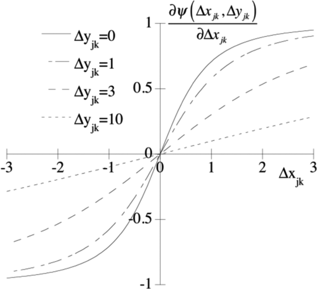
For simplicity, consider the case where δ and η are 1. Fig. 1 shows a plot of the derivative of the potential function for several different values of Δy_jk. Note that the “force” increases more rapidly as a function of the difference in the pixel values in the x image when the difference in pixel values in the y image is smaller. Thus, small differences in the pixel values of neighboring pixels y in the image favor small differences in the pixel values in the x image. Similarly, large differences in neighboring pixel values in the y image apply less “force” to smooth differences in the pixels in the x image. In other words, if the differences in both the y image and x image are small, then the partial derivative is large, and the prior will provide more smoothing. On the other hand, if the differences in both the y and x images are large, then the partial derivative will be small, providing less smoothing. When the difference in one image is large but small in the other image, the smoothing will be somewhere in between the previous two cases.

Fig. 1.

Graph of partial derivative of cross-tracer prior potential function with respect to pixel differences in the x image for various values of pixel difference in the y image.

F. Convergent PML Algorithm With the Cross-Tracer Prior Separable Surrogate Function of the Prior

To obtain a closed-form solution for the update equation, we first construct a separable surrogate function for the penalty function at a given iteration using the estimate obtained from the previous iteration. The surrogate function is denoted by Λ⁽ⁿ⁾ (x, y), and should satisfy the following conditions:

$$\begin{array}{cc}\mathrm{C}1)\hfill & {\mathrm{\Lambda }}^{(n)}({\mathbf{x}}^{(n)},{\mathbf{y}}^{(n)})=\mathrm{\Lambda }({\mathbf{x}}^{(n)},{\mathbf{y}}^{(n)})\hfill \end{array}$$ (8)

and

$$\begin{array}{cc}\mathrm{C}2)\hfill & {\mathrm{\Lambda }}^{(n)}(\mathbf{x},\mathbf{y})\ge \mathrm{\Lambda }(\mathbf{x},\mathbf{y})\text{ for all }\mathbf{x}\text{ and }\mathbf{y}\hfill \end{array}$$ (9)

where xⁿ and y⁽ⁿ⁾ are the estimates of x and y after the nth iteration.

We now derive the separable surrogates for the hyperbolic prior function in (5). Let

$$\psi (x_j,x_k,y_j,y_k)=\lambda (x_j-x_k,y_j-y_k)$$ (10)

and define

$${\lambda }_x^{\prime }(x,y)=\frac{\partial \lambda (x,y)}{\partial x}$$

and

$${\lambda }_y^{\prime }(x,y)=\frac{\partial \lambda (x,y)}{\partial y}.$$ (11)

Further, let

$${\gamma }_x(x,y)=\frac{\partial \lambda (x,y)}{\partial x}·\frac{1}{x}$$

and

$${\gamma }_y(x,y)=\frac{\partial \lambda (x,y)}{\partial y}·\frac{1}{y}.$$ (12)

Given the above assumptions, in Appendix I we derived a separable surrogate function, Λ⁽ⁿ⁾ (x, y), given by

$${\mathrm{\Lambda }}^{(n)}(\mathbf{x},\mathbf{y})={\mathrm{\Lambda }}_{\mathbf{x}}^{(n)}(\mathbf{x})+{\mathrm{\Lambda }}_{\mathbf{y}}^{(n)}(\mathbf{y})+C^{(n)}$$ (13)

where

$$\begin{array}{c}{\mathrm{\Lambda }}_{\mathbf{x}}^{(n)}(\mathbf{x})=2{\displaystyle \sum _{j=1}^J}{\displaystyle \sum _{k\in N_j}}{h}_{\mathit{\text{jk}}}^{(n)}(x_j)\hfill \\ {\mathrm{\Lambda }}_{\mathbf{x}}^{(n)}(\mathbf{x})=2{\displaystyle \sum _{j=1}^J}{\displaystyle \sum _{k\in N_j}}{h}_{\mathit{\text{jk}}}^{(n)}(x_j)\hfill \end{array}$$ (14)

and

$$\begin{array}{c}{\mathrm{\Lambda }}_{\mathbf{y}}^{(n)}(\mathbf{y})=2{\displaystyle \sum _{j=1}^J}{\displaystyle \sum _{k\in N_j}}{g}_{\mathit{\text{jk}}}^{(n)}(y_j)\hfill \\ {\mathrm{\Lambda }}_{\mathbf{y}}^{(n)}(\mathbf{y})=2{\displaystyle \sum _{j=1}^J}{\displaystyle \sum _{k\in N_j}}{g}_{\mathit{\text{jk}}}^{(n)}(y_j)\hfill \end{array}$$ (15)

where C⁽ⁿ⁾ is a constant independent of x and y

$$h_{\mathit{\text{jk}}}^{(n)}(x)={\omega }_{\mathit{\text{jk}}}{\gamma }_x\left(x_j^{(n)}-x_k^{(n)},y_j^{(n)}-y_k^{(n)}\right)\times {\left(x-\frac{x_j^{(n)}+x_k^{(n)}}{2}\right)}^2$$ (16)

and

$$g_{\mathit{\text{jk}}}^{(n)}(y)={\omega }_{\mathit{\text{jk}}}{\gamma }_y\left(x_j^{(n)}-x_k^{(n)},y_j^{(n)}-y_k^{(n)}\right)\times {\left(y-\frac{y_j^{(n)}+y_k^{(n)}}{2}\right)}^2.$$ (17)

G. Surrogate Function for the Log Likelihood Functions

De Pierro derived a surrogate function for the log likelihood function [7], [19]. Chang et al. later adopted this surrogate function to develop a convergent PML algorithm for PET image reconstruction [10]. This surrogate function, $L_{\mathbf{x}}^{(n)}$, is given by

$$L_{\mathbf{x}}^{(n)}(\mathbf{x})={\displaystyle \sum _{i=1}^I}\left\{{\displaystyle \sum _{j=1}^J}{P}_{\mathit{\text{ij}}}\frac{p_i{x}_j^{(n)}}{{\displaystyle \sum _{k=1}^J}{P}_{\mathit{\text{ik}}}{x}_k^{(n)}}\text{log}{x}_j-{\displaystyle \sum _{j=1}^J}{P}_{\mathit{\text{ij}}}{x}_j\right\}+C_{1,L_x}^{(n)}$$ (18)

where the constant $C_{1,L_x}^{(n)}$ is independent of x_j. In (18), P_ij denotes the probability that a photon emitted from the jth voxel of image x is detected in the ith detector bin, and p_i is the observed projection data from image x in the ith detector bin. It has been shown [7], [10], that

$$\begin{array}{ccc}\mathrm{C}1)\hfill & L_{\mathbf{x}}^{(n)}({\mathbf{x}}^{(n)})=L_{\mathbf{x}}({\mathbf{x}}^{(n)})\hfill & \text{and}\hfill \end{array}$$ (19)

$$\begin{array}{cc}\mathrm{C}2)\hfill & L_{\mathbf{x}}^{(n)}(\mathbf{x})\le L_{\mathbf{x}}(\mathbf{x})\text{ for all }\mathbf{x}.\hfill \end{array}$$ (20)

Note that (18) does not include additive terms to model crosstalk, but these could be easily incorporated.

H. Surrogate Function for the Objective Function

The goal is to derive a separable surrogate function for the objective function in (1). We have obtained the surrogate functions for both the log likelihood functions and the prior. The surrogate for the objective function in (1) is thus the sum of these two surrogate functions, i.e.,

$${\mathrm{\Phi }}^{(n)}(\mathbf{x},\mathbf{y})=-L_{\mathbf{x}}^{(n)}(\mathbf{x})-L_{\mathbf{y}}^{(n)}(\mathbf{y})+\beta {\mathrm{\Lambda }}_{\mathbf{x}}^{(n)}(\mathbf{x})+\beta {\mathrm{\Lambda }}_{\mathbf{y}}^{(n)}(\mathbf{y})+\beta C^{(n)}-C_{1,L_x}^{(n)}-C_{1,L_y}^{(n)}.$$ (21)

Considering equations (8) and (9) and (19) and (20), it can be proved that the surrogate objective function Φ⁽ⁿ⁾ (x, y) in (21) satisfies the following conditions:

$$\mathrm{C}1){\mathrm{\Phi }}^{(n)}({\mathbf{x}}^{(n)},{\mathbf{y}}^{(n)})=\mathrm{\Phi }({\mathbf{x}}^{(n)},{\mathbf{y}}^{(n)})$$ (22)

and

$$\mathrm{C}2){\mathrm{\Phi }}^{(n)}(\mathbf{x},\mathbf{y})\ge \mathrm{\Phi }(\mathbf{x},\mathbf{y})\text{ for all }\mathbf{x}\text{ and }\mathbf{y}.$$ (23)

Substituting the surrogate functions of the log likelihood functions and the priors into (1), we obtain the separable surrogate function of Φ(x, y), i.e.,

$${\mathrm{\Phi }}^{(n)}(\mathbf{x},\mathbf{y})={\mathrm{\Phi }}_{\mathbf{x}}^{(n)}(\mathbf{x})+{\mathrm{\Phi }}_{\mathbf{y}}^{(n)}(\mathbf{y})+C^{(n)}+C_{1,L_x}^{(n)}+C_{1,Ly}^{(n)}$$ (24)

where

$${\mathrm{\Phi }}_{\mathbf{x}}^{(n)}(\mathbf{x})=-L^{(n)}(\mathbf{x})+\beta {\mathrm{\Lambda }}^{(n)}(\mathbf{x})=-{\displaystyle \sum _{i=1}^I}\left\{{\displaystyle \sum _{j=1}^J}{p}_i\frac{P_{\mathit{\text{ij}}}{x}_j^{(n)}}{{\displaystyle \sum _{k=1}^J}{P}_{\mathit{\text{ik}}}{x}_k^{(n)}}\text{log}{x}_j-{\displaystyle \sum _{k=1}^J}{P}_{\mathit{\text{ik}}}{x}_k\right\}+2\beta {\displaystyle \sum _{j=1}^J}{\displaystyle \sum _{k\in N_j}}{h}_{\mathit{\text{jk}}}^{(n)}(x_j)$$ (25)

and

$${\mathrm{\Phi }}_{\mathbf{y}}^{(n)}(\mathbf{y})=-L^{(n)}(\mathbf{y})+\beta {\mathrm{\Lambda }}^{(n)}(\mathbf{y})=-{\displaystyle \sum _{i=1}^I}\left\{{\displaystyle \sum _{j=1}^J}{q}_i\frac{H_{\mathit{\text{ij}}}{y}_j^{(n)}}{{\displaystyle \sum _{k=1}^J}{H}_{\mathit{\text{ik}}}{y}_k^{(n)}}\text{log}{y}_j-{\displaystyle \sum _{k=1}^J}{H}_{\mathit{\text{ik}}}{y}_k\right\}+2\beta {\displaystyle \sum _{j=1}^J}{\displaystyle \sum _{k\in N_j}}{g}_{\mathit{\text{jk}}}^{(n)}(y_i).$$ (26)

The surrogate functions (25) and (26) are separable in terms of x and y. Thus one can minimize Φ⁽ⁿ⁾ (x, y) simply by minimizing ${\mathrm{\Phi }}_{\mathbf{x}}^{(n)}(\mathbf{x})\text{ and }{\mathrm{\Phi }}_{\mathbf{y}}^{(n)}(\mathbf{y})$ separately. In (26), H_ij is the probability that a photon emitted from the jth voxel of image y is detected in the ith detector bin, and q_i is the observed projection data from image y in the ith detector bin. Note that H_ij differs from P_ij because the attenuation and scatter are different for the two tracers.

I. Derivation of the Convergent PML Algorithm

From the decoupled objective functions, one can solve for x and y by minimizing (25) and (26) separately. First consider the minimization problem for ${\mathrm{\Phi }}_{\mathbf{x}}^{(n)}(\mathbf{x})$ in (25). Substituting (16) into (25), ${\mathrm{\Phi }}_{\mathbf{x}}^{(n)}(\mathbf{x})$ becomes

$${\mathrm{\Phi }}_{\mathbf{x}}^{(n)}(\mathbf{x})=-{\displaystyle \sum _{i=1}^I}{\displaystyle \sum _{j=1}^J}{p}_i\frac{P_{\mathit{\text{ij}}}{x}_j^{(n)}}{{\displaystyle {\sum }_{k=1}^J}{P}_{\mathit{\text{ik}}}{x}_k^{(n)}}\text{log}{x}_j+{\displaystyle \sum _{i=1}^I}{\displaystyle \sum _{k=1}^J}{P}_{\mathit{\text{ik}}}{x}_k+2\beta {\displaystyle \sum _{j=1}^J}{\displaystyle \sum _{k\in N_j}}{\omega }_{\mathit{\text{jk}}}{\gamma }_x(x_j^{(n)}-x_k^{(n)},y_j^{(n)}-y_k^{(n)})x_j^2-2\beta {\displaystyle \sum _{j=1}^J}{\displaystyle \sum _{k\in N_j}}{\omega }_{\mathit{\text{jk}}}{\gamma }_x(x_j^{(n)}-x_k^{(n)},y_j^{(n)}-y_k^{(n)})\times (x_j^{(n)}+x_k^{(n)})x_j+\frac{1}{2}\beta {\displaystyle \sum _{j=1}^J}{\displaystyle \sum _{k\in N_j}}{\omega }_{\mathit{\text{jk}}}{\gamma }_x(x_j^{(n)}-x_k^{(n)},y_j^{(n)}-y_k^{(n)})\times {(x_j^{(n)}+x_k^{(n)})}^2.$$ (27)

Simplifying, we have

$${\mathrm{\Phi }}_{\mathbf{x}}^{(n)}(\mathbf{x})=-{\displaystyle \sum _{j=1}^J}{E}_j^{(n)}\text{log}{x}_j+{\displaystyle \sum _{j=1}^J}{G}_j^{(n)}{x}_j+{\displaystyle \sum _{j=1}^J}{F}_j^{(n)}{x}_j^2={\displaystyle \sum _{j=1}^J}\left[-E_j^{(n)}\text{log}{x}_j+G_j^{(n)}{x}_j+F_j^{(n)}{x}_j^2\right]$$ (28)

where

$$E_j^{(n)}={\displaystyle \sum _{i=1}^I}{p}_i\frac{P_{\mathit{\text{ij}}}{x}_j^{(n)}}{{\displaystyle \sum _{k=1}^J}{P}_{\mathit{\text{ik}}}{x}_k^{(n)}},$$ (29)

$$F_j^{(n)}=2\beta {\displaystyle \sum _{k\in N_i}}{\omega }_{\mathit{\text{jk}}}{\gamma }_x(x_j^{(n)}-x_k^{(n)},y_j^{(n)}-y_k^{(n)})$$ (30)

and

$$G_j^{(n)}={\displaystyle \sum _{i=1}^I}{P}_{\mathit{\text{ij}}}-2\beta {\displaystyle \sum _{k\in N_i}}{\omega }_{\mathit{\text{jk}}}{\gamma }_x\times \left(x_j^{(n)}-x_k^{(n)},y_j^{(n)}-y_k^{(n)}\right)(x_j^{(n)}+x_k^{(n)}).$$ (31)

Now we can find the optimal solution for x_j, that is

$$x_j^{(n+1)}=\text{arg}\underset{x_j\ge 0}{\text{min}}{s}_j^{(n)}(x_j)j=1,2,\dots J$$ (32)

where

$$s_j^{(n)}(t)=-E_j^{(n)}\text{log}t+G_j^{(n)}t+F_j^{(n)}{t}^2.$$ (33)

Since the second derivative of $s_j^{(n)}(t)$ is non-negative, i.e.,

$$\frac{{\partial }^2{s}_j^{(n)}(t)}{\partial t^2}=E_j^{(n)}\frac{1}{t^2}+2F_j^{(n)}>0$$ (34)

the function $s_j^{(n)}(t)$ is convex. Finding the solution for (32) is equivalent to solving the following equation:

$$\frac{\partial s_j^{(n)}(t)}{\partial t}=-\frac{E_j^{(n)}}{t}+G_j^{(n)}+2F_j^{(n)}t=0.$$ (35)

The solution to (32) is thus

$$x_j^{(n+1)}=\frac{-G_j^{(n)}+\sqrt{G_j^{(n)2}+8F_j^{(n)}{E}_j^{(n)}}}{4F_j^{(n)}}.$$ (36)

Similarly, we derived the solution for $y_j^{(n+1)}$

$$y_j^{(n+1)}=\frac{-G_j^{\prime (n)}+\sqrt{G_j^{\prime (n)2}+8F_j^{\prime (n)}{E}_j^{\prime (n)}}}{4F_j^{\prime (n)}}$$ (37)

where

$$E_j^{\prime (n)}={\displaystyle \sum _{i=1}^I}{q}_i\frac{H_{\mathit{\text{ij}}}{y}_j^{(n)}}{{\displaystyle \sum _{k=1}^J}{H}_{\mathit{\text{ik}}}{y}_k^{(n)}}$$ (38)

$$F_j^{\prime (n)}=2\beta {\displaystyle \sum _{k\in N_j}}{\omega }_{\mathit{\text{jk}}}{\gamma }_y(x_j^{(n)}-x_k^{(n)},y_j^{(n)}-y_k^{(n)})$$ (39)

and

$$G_j^{\prime (n)}={\displaystyle \sum _{i=1}^I}{H}_{\mathit{\text{ij}}}-2\beta {\displaystyle \sum _{k\in N_j}}{\omega }_{\mathit{\text{jk}}}{\gamma }_y\times \left(x_j^{(n)}-x_k^{(n)},y_j^{(n)}-y_k^{(n)}\right)\left(y_j^{(n)}+y_k^{(n)}\right).$$ (40)

(36)–(40) are the MAP algorithm. Note that in deriving (36) and (37), we excluded the negative solutions.

J. Accelerated PML Algorithms Using Ordered Subsets

The algorithm derived in the previous section converges to the MAP solution; however, it is slow without using ordered subset techniques. Direct application of ordered subsets would accelerate the reconstruction process, but the resulting algorithm would not be guaranteed to converge. We have thus derived a convergent ordered-subset algorithm based on the work in [12], [20] and COSEM [5], [15]–[17], both of which are particular examples of incremental EM algorithm [13]. In [21], incremental optimization transfer, as a generalization of the incremental EM algorithm, was applied to transmission tomography. The incremental EM algorithm is a generalization of ordinary EM, generalizing from expectation-maximization to maximization-maximization. That is, the E step in the ordinary EM algorithm is replaced by a maximization procedure. This variant of the EM algorithm is applicable to the case of statistically independent observations, and thus to the case of emission tomography. The algorithm divides the observed data and complete data into partitions (ordered-subsets), and there are two sub-iterations for each iteration. In the first sub-iteration, optimization is achieved by updating the conditional sufficient statistics with complete data on one partition only. In the second step, the parameters, in our case the image estimates, are chosen to optimize the conditional expectation of the likelihood of all the complete data. For more details, refer to the discussions in [12], [13], and [20]. In emission tomography, the elements of the complete data are the number of emissions from each voxel detected by one particular detector bin, which is also a component of the sufficient statistics vector; the observed data is the number of emissions from all pixels detected in one detector bin; and the parameters to be estimated are the activity in each voxel. As a particular example of incremental EM algorithm, COSEM formulates the reconstruction problem as an optimization problem with respect to both the image estimate and complete data, which is solved by alternate updating of the image estimates and complete data. In particular, in the COSEM-MAP framework, the objective function for the complete data is formulated using ordered-subsets as [15], [21]

$$E_{\text{cmp}-\text{MAP}}(\mathbf{C},\mathbf{x},\mathbf{v})=E_{\text{cmp}-\text{ML}}(\mathbf{C},\mathbf{x},\mathbf{v})+\beta \mathrm{\Psi }(\mathbf{x})={\displaystyle \sum _{\mathit{\text{ij}}}}{P}_{\mathit{\text{ij}}}{x}_j+{\displaystyle \sum _{l=1}^L}{\displaystyle \sum _{i\in S_l}}{\displaystyle \sum _{j=1}^N}{C}_{\mathit{\text{ij}}}\text{ log }\frac{C_{\mathit{\text{ij}}}}{P_{\mathit{\text{ij}}}{x}_j}-{\displaystyle \sum _{l=1}^L}{\displaystyle \sum _{i\in S_l}}{\displaystyle \sum _{j=1}^N}{C}_{\mathit{\text{ij}}}+{\displaystyle \sum _i}{\upsilon }_i\left({\displaystyle \sum _j}{C}_{\mathit{\text{ij}}}-p_i\right)+\beta \mathrm{\Psi }(\mathbf{x})$$ (41)

where C_ij is the (i, j)th element of the complete data, ν_i is a Lagrange multiplier to add the constraint ∑_j C_ij = p_i, where p_i is the projection data in the ith bin, Ψ(x) is the potential function of the prior and s_l is the lth subset. In [14], a separable surrogate was derived for a quadratic prior. The optimization of (41) uses an alternating descent approach and performs the reconstruction using two update equations: 1) a complete data update and 2) an image estimate update.

Here we extend (41) to the joint estimation problem for the cross-tracer prior. Rewriting (1) using the surrogate function for the cross-tracer prior we get

$$E(\mathbf{C},\mathbf{C}\prime ,\mathbf{x},\mathbf{y},\mathbf{v},\mathbf{v}\prime )=E_{\text{cmp}-\text{ML}}(\mathbf{C},\mathbf{x},\mathbf{v})+E_{\text{cmp}-\text{ML}}(\mathbf{C}\prime ,\mathbf{y},\mathbf{v}\prime )+\mathrm{\Lambda }(\mathbf{x},\mathbf{y})$$ (42)

where C and C′ are the complete data matrices for images x and y, respectively, and v and v′ are the Lagrange multipliers for the constraints ∑_j C_ij = p_i and ∑_j C′_ij = q_i, respectively.

The first step of the optimization is the complete data update. Taking partial derivatives with respect to the elements in C and C′, solving for the maximum, and enforcing the constraints results in

$$C_{\mathit{\text{ij}}}^{(n,l)}=p_i\frac{P_{\mathit{\text{ij}}}{x}_j^{(n,l-1)}}{{\displaystyle \sum _k}{P}_{\mathit{\text{ik}}}{x}_k^{(k,l-1)}},\forall i\in S_l,\forall j$$ (43)

$$C_{\mathit{\text{ij}}}^{(n,l)}=C_{\mathit{\text{ij}}}^{(n,l-1)},\forall i\notin S_l,\forall j$$ (44)

$$C_{\mathit{\text{ij}}}^{\prime (n,l)}=q_i\frac{H_{\mathit{\text{ij}}}{x}_j^{(n,l-1)}}{{\displaystyle \sum _k}{H}_{\mathit{\text{ik}}}{x}_k^{(n,l-1)}},\forall i\in S_l,\forall j$$ (45)

and

$$C_{\mathit{\text{ij}}}^{\prime (n,l)}=C_{\mathit{\text{ij}}}^{\prime (n,l-1)},\forall i\notin S_l,\forall j$$ (46)

where the superscript (n, l) denotes the nth iteration and lth subset.

The second step in the optimization is updating the image estimates, x and y, with the complete data fixed. To do this, we replaced the prior with the separable surrogate function. Following the derivation in [14] and [17], in this step we used the objective

$$E_{\mathit{\text{obj}}}({\mathbf{x}}^{(n,l)},{\mathbf{y}}^{(n,l)})=-{\displaystyle \sum _{m=1}^L}{\displaystyle \sum _{i\in S_m}}{\displaystyle \sum _{j=1}^N}{C}_{\mathit{\text{ij}}}^{(n,l)}\text{ log }{P}_{\mathit{\text{ij}}}{x}_j+{\displaystyle \sum _{\mathit{\text{ij}}}}{P}_{\mathit{\text{ij}}}{x}_j-{\displaystyle \sum _{m=1}^L}{\displaystyle \sum _{i\in S_m}}{\displaystyle \sum _{j=1}^N}{C}_{\mathit{\text{ij}}}^{\prime (n,l)}\text{ log }{H}_{\mathit{\text{ij}}}{y}_j+{\displaystyle \sum _{\mathit{\text{ij}}}}{H}_{\mathit{\text{ij}}}{y}_j+2\beta {\displaystyle \sum _{j=1}^J}{\displaystyle \sum _{k\in N_j}}{h}_{\mathit{\text{jk}}}^{(n,l)}(x_j)+C_{\mathbf{x}}^{(n,l)}+2\beta {\displaystyle \sum _{j=1}^J}{\displaystyle \sum _{k\in N_j}}{g}_{\mathit{\text{jk}}}^{(n,l)}(x_j)+C_{\mathbf{y}}^{(n,l)}$$ (47)

where $g_{\mathit{\text{jk}}}^{(n,l)}(x)\text{ and }{h}_{\mathit{\text{jk}}}^{(n,l)}(x)$ are defined similar to those in (16) and (17), and $C_x^{(n,l)}\text{ and }{C}_y^{(n,l)}$ are constants that do not depend on x^{(n, l)} and y^{(n, l)}. Minimization of (47) can thus be achieved by minimizing the terms involving x and y separately to obtain the solution to x^{(n, l)} and y^{(n, l)}. In particular, taking the partial derivatives of (47) with respect to x_j and y_j separately, equating to zero, and solving, we obtain

$$\{\begin{array}{cc}{x}_j^{(n,l)}\hfill & =\frac{-G_j^{(n,l-1)}+\sqrt{{\left(G_j^{(n,l-1)}\right)}^2+16\beta F_j^{(n,l-1)}{E}_j^{(n,l)}}}{8\beta F_j^{(n,l-1)}}\hfill \\ y_j^{(n,l)}\hfill & =\frac{-G_j^{\prime (n,l-1)}+\sqrt{{\left(G_j^{\prime (n,l-1)}\right)}^2+16\beta F_j^{\prime (n,l-1)}{E}_j^{\prime (n,l)}}}{8\beta F_j^{\prime (n,l-1)}}\hfill \end{array}$$ (48)

where

$$\begin{array}{c}{E}_j^{(n,l)}={\displaystyle \sum _i}{C}_{\mathit{\text{ij}}}^{(n,l)}\hfill \\ F_j^{(n,l-1)}={\displaystyle \sum _{k\in N_j}}\left\{{\omega }_{\mathit{\text{jk}}}{\gamma }_x\right(x_j^{(n,l-1)}-x_k^{(n,l-1)},y_j^{(n,l-1)}-y_k^{(n,l-1)}\left)\right\}\hfill \\ G_j^{(n,l-1)}={\displaystyle \sum _i}{P}_{\mathit{\text{ij}}}-2\beta {\displaystyle \sum _{k\in N_j}}{\omega }_{\mathit{\text{jk}}}{\gamma }_x\left(x_j^{(n,l-1)}-x_k^{(n,l-1)},y_j^{(n,l-1)}-y_k^{(n,l-1)}\right)(x_j^{(n,l-1)}+x_k^{(n,l-1)})\hfill \\ E_j^{\prime (n,l)}={\displaystyle \sum _i}{C}_{\mathit{\text{ij}}}^{\prime (n,l)}\hfill \\ F_j^{\prime (n,l-1)}={\displaystyle \sum _{k\in N_j}}\left\{{\omega }_{\mathit{\text{jk}}}{\gamma }_y\right(x_j^{(n,l-1)}-x_k^{(n,l-1)},y_j^{(n,l-1)}-y_k^{(n,l-1)}\left)\right\}\hfill \end{array}$$

and

$$G_j^{\prime (n,l-1)}={\displaystyle \sum _i}{H}_{\mathit{\text{ij}}}-2\beta {\displaystyle \sum _{k\in N_j}}{\omega }_{\mathit{\text{jk}}}{\gamma }_y\left(x_j^{(n,l-1)}-x_k^{(n,l-1)},y_j^{(n,l-1)}-y_k^{(n,l-1)}\right)\left(y_j^{(n,l-1)}+y_k^{(n,l-1)}\right).$$

In summary, the dual-isotope reconstruction using the cross-tracer prior based on COSEM framework is implemented in two steps. Step 1 updates the complete data using (43)–(46), and Step 2 updates the images using (48).

II. Evaluation Experiments

A. Comparison Using Sample Images

We have investigated the convergence of the proposed algorithm and the qualitative properties of the reconstructed images using a simulation study. Projection data were simulated using the 4D NCAT torso phantom. A defect was placed on the myocardial wall. Low noise projection data were simulated using the SimSET Monte Carlo simulation code. The projection data were scaled and Poisson noise was added to obtain projections with a clinically realistic noise level. We used these data to perform experiments demonstrating the convergence of the algorithm and the properties of the cross-tracer prior.

B. Image Fidelity Study

To investigate the properties and benefits of the cross-tracer prior we performed a simulation experiment using a phantom designed to simulate myocardial perfusion imaging while being simple enough to provide insight into the effects of the reconstruction hyperparameters. The phantom consisted of an elliptical cylinder 16 cm long with major and minor axes of 31 and 21 cm, respectively. A spherical shell with outside and inside diameters of 8 and 5 cm, respectively, was created to simulate the myocardium. The shell was offset 4 cm in the left lateral direction and 2 cm in the anterior direction from the center of the cylinder. The shell had an activity 5 times as high as the background. We created a simulated perfusion defect with a 50% reduction of myocardial activity in the region of intersection of a 4 cm diameter sphere centered in the middle of the shell wall at the left lateral position. We created a pair of phantoms representing a reversible defect: one without the defect (rest) and one with the defect (stress). The phantoms were digitized into 64 × 64 × 32 cm matrices with a voxel size of 0.5 cm. We also created an attenuation map the same size as the cylinder with an attenuation coefficient of 0.15 cm⁻¹. We used the same analytic projector as used in the reconstruction to generate projections for a standard 180° cardiac orbit with 64 projection views. We modeled an LEHR collimator (including spatially varying blurring) and a circular radius of rotation of 16 cm. The projections were scaled to a total of 100 k counts in the central slice of the phantom and Poisson noise was simulated. The images were reconstructed using OS-EM (up to 20 iterations with 16 subsets per iteration), the proposed MAP algorithm with the cross-tracer prior (CTMAP), and the same algorithm modified to use only the hyperbolic prior applied to each of the images separately. In other words, we used the prior

$$\mathrm{\Lambda }(\mathbf{x})={\displaystyle \sum _j^J}{\displaystyle \sum _{k\in N_j}}{\omega }_{\mathit{\text{jk}}}\sqrt{1+{\left(\frac{x_j-x_k}{\delta }\right)}^2}-1.$$ (49)

for the x an y images, which were reconstructed separately. A total of 100 iterations (16 subsets per iteration) were used for the MAP reconstruction to insure convergence. All reconstructions were performed with attenuation and collimator-detector response modeling. The OS-EM images were postreconstruction filtered using Butterworth filters with an order 8 and cutoff frequencies from 0.10 to 0.30 pixel⁻¹ in increments of 0.02 pixels⁻¹. For the MAP methods, we investigated values of β equal to 5, 2, and 1 times 10ⁿ, with n in the range 0 to −4, for a total of 12 values of β. For each β we used values of δ^1/2 equal to 0.01, 0.02, 0.05, 0.1, 0.2, 0.5, and 1.0, and used the same value of δ for both images (i.e., set η = δ for CTMAP).

After reconstruction and (for OS-EM) filtering, we computed the voxel-by-voxel mean-square error with respect to the phantom to provide a measure of image fidelity.

C. Task-Based Three-Class Observer Study

To evaluate the proposed algorithms in the context of reconstructing dual-isotope images, we conducted a three-class observer study to evaluate the classification performance in distinguishing between patients with no defect, with a reversible defect, or with a fixed defect. In this study, we used a population of stress (^99mTc) and rest (²⁰¹Tl) images that realistically modeled patient variations.

In this study we used a previously developed phantom population [4], [22] based on the 4D NCAT phantom [23], which realistically modeled the anatomical and organ uptake variations seen in clinical data. The phantom population included 24 NCAT anatomies with variations in gender, patient size, heart angle, size, and position, and lung volume [24]. We modeled variations in perfusion defect sizes and locations. Please refer to [4], [22], [25] for the details of the phantom population generation.

For each of the 24 anatomies, we separately simulated projections of five organs (heart, lung, body, liver, and kidney) using a combined SimSET and angular response function (ARF) simulation code [26]. Attenuation, scatter in the body, the distant-dependent collimator-detector response, and penetration and scatter in the collimator were modeled in the simulation. Data for ²⁰¹Tl were simulated including the seven major emission energies. The energy window for ^99mTc was 15% wide, centered at 140.5 KeV; that for ²⁰¹Tl was 20% wide, centered at 70 KeV. Square projection bins and cubic reconstructed voxels with a side length of 0.48 cm were used for both ^99mTc and ²⁰¹Tl images. The projections consisted of 64 views over 180° from left posterior oblique (LPO) to right anterior oblique (RAO). Since the phantoms modeled uptakes observed in real patients, and the simulations modeled the sensitivity and acquistion times for clinical cardiac acquisitions, the count levels in the data were clinically realistic for both isotopes. The means ± standard deviations of the total counts in the sinogram averaged over the 48 slices reconstructed were 193 ± 38 k counts for ^99mTc and 110±26 k counts for ²⁰¹Tl.

Using the individual projections, we generated a population of dual-isotope projection data that included realistic variations in organ uptake by summing the organ projections. Defects at three locations in the myocardium were simulated. The projection data were scaled to model ^99mTc and ²⁰¹Tl injected activities of 16 and 3 mCi, respectively. This procedure produced 1296 pairs of ^99mTc/²⁰¹Tl projection datasets (24 phantoms × 3 defect locations × 6 uptake ratio combinations × 3 defect statuses, i.e., normal, reversible defect, and fixed defect). Note that we did not include crosstalk in these simulations because the implementation of the cross-tracer MAP reconstruction algorithm did not include the ability to compensate for crosstalk. The inclusion of crosstalk in the data combined with use of crosstalk compensation would result in increased noise in the reconstructed images, especially for ²⁰¹Tl. This should provide a greater advantage for the cross tracer prior, but this requires future in depth investigation.

We reconstructed the 1,296 pairs of ^99mTc/²⁰¹Tl images using the proposed algorithm. In the reconstruction process, attenuation and detector response effects (AD) were modeled. As a comparison, we performed OS-EM reconstruction with the same compensations. In both cases we used 20 iterations with 16 updates per iteration.

We then applied standard postprocessing methods to the reconstructed images. For OS-EM reconstruction, the images were reoriented to short axis, filtered with a Butterworth filter, and windowed to obtain short axis (SA) ^99mTc/²⁰¹Tl image pairs. For each reoriented 3D stress (^99mTc) image, a 32 × 32 image containing the centroid of the defect (or the same short-axis slice in the corresponding defect-absent image) was extracted from the postprocessed short-axis slices. The same short-axis slice in the corresponding rest (²⁰¹Tl) image was also selected. These ^99mTc/²⁰¹Tl SA image pairs served as the input for the three-class mathematical observer studies. For the cross-tracer MAP reconstruction, the same postprocessing methods were used with the exception that the Butterworth filtering was omitted.

We then applied a three-class channelized Hotelling observer (3-CHO) to the ^99mTc/²⁰¹Tl image pair, resulting in one feature vector for each image pair. The details for the 3-CHO and the channels used for the 3-CHO are described in [4].

Using half the image pairs for each reconstruction and post-processing combination, we trained a 3-CHO, which was then tested using the remaining half of the images. The volume under a three-class ROC surface (VUS) was used as a figure-of-merit for task performance.

III. Results

A. Convergence of the Two Algorithms

We verified the convergence of the convergent and accelerated PML algorithms for the cross-tracer prior, introduced in Sections I-I and I-J, using the following parameters: $\delta =\eta =\sqrt{10}$ and β = 0.05.

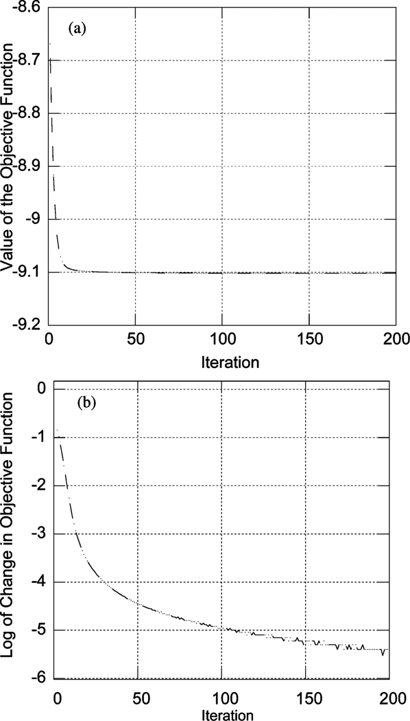
We evaluated the value of the objective function in (1) at each iteration for the convergent PML algorithm, as shown in Fig. 2(a). Also shown is the (negative) change of objective function on a semi-log scale. In particular, we computed ln(−(ϕ(i + 1) − ϕ(i))), where ϕ(i) is the objective function evaluated at the ith iteration. These data show that, as expected, the objective function decreases monotonically.

Fig. 2.

(a) Plot of the objective function and (b) logarithm of the (negative) change of the objective function of the convergent PML algorithm as a function of iteration.

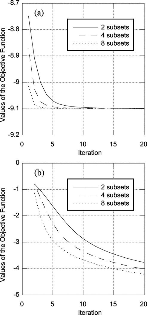
Using the same set of parameters, we tested the convergence of the accelerated PML algorithms. As noted in [12], [15], [20], the energy function defined in (42) decreases monotonically with each iteration, and the algorithm reaches the maximum a posterior (MAP) solution of (1), though a monotonic decrease of the objective function in (1) is not guaranteed. Despite this, in our simulations we did observe a monotonic decrease in the objective function of (1). Fig. 3 shows the value of the objective function for three values of the number of subsets per iteration (8, 4, and 2), corresponding to 8, 16, and 32 angles per subset, respectively. It can be seen that the accelerated algorithm converged faster with a smaller number of angles per subset (i.e., more subsets per iteration). In addition, the accelerated algorithm achieved the same ultimate value of the objective function.

Fig. 3.

Plot of the value of objective functions (a) and logarithm of the (negative) change of the objective functions of the accelerated PML algorithm as a function of iteration for 2, 4, and 8 subsets per iteration.

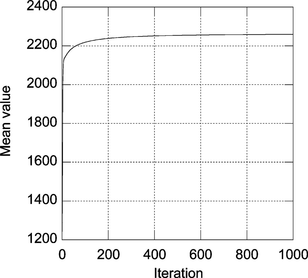
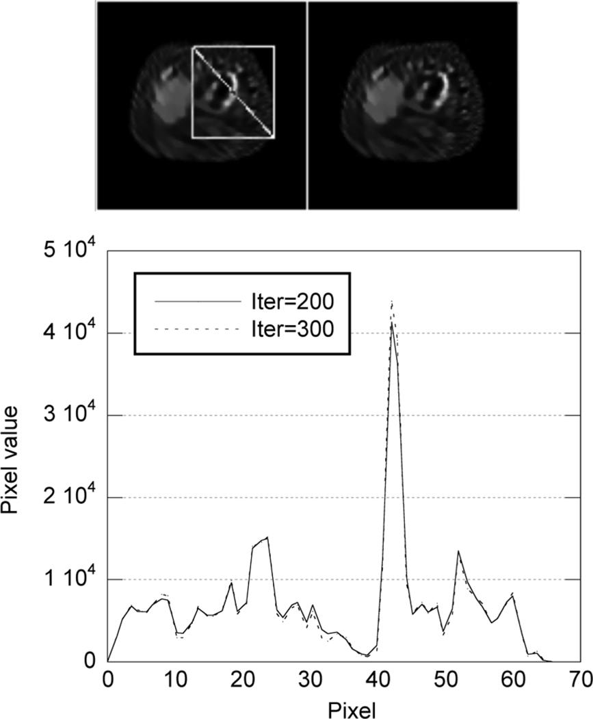
We have also studied the change of mean value of three slices of the reconstructed images with iterations to demonstrate the convergence of the convergent PML algorithm. The results are shown in Fig. 4. It can be seen that convergence is achieved after 200 iterations. A comparison of images and profiles through the Tc-99m stress images after 200 and 300 iterations is shown in Fig. 5. These data demonstrate that both the value of the objective function and the reconstructed images converge.

Fig. 4.

The mean value of the reconstructed images with iterations.

Fig. 5.

Profiles of stress images at iteration 200 and 300.

B. Effects of the Cross-Tracer Prior—Comparison of Sample Images

Using the parameters in the previous section, we reconstructed a pair of images that contained reversible defects to demonstrate the effects of the cross-tracer prior compared to a conventional edge-preserving prior. The conventional edge-preserving prior used is that shown in (49). This reconstruction algorithm will be referred to as single-tracer MAP (STMAP). We used the same value of β and δ for both the rest and stress images and the same values used in the previous section $(\beta =0.05,\delta =\sqrt{10})$. We used a set of projection data with a reversible defect (defect present in the stress image, but not in the rest image) with a reduction of 35% of the myocardial activity concentration. We generated and reconstructed 50 sets of simulated Poisson noise realizations and computed both the mean and standard deviation images.

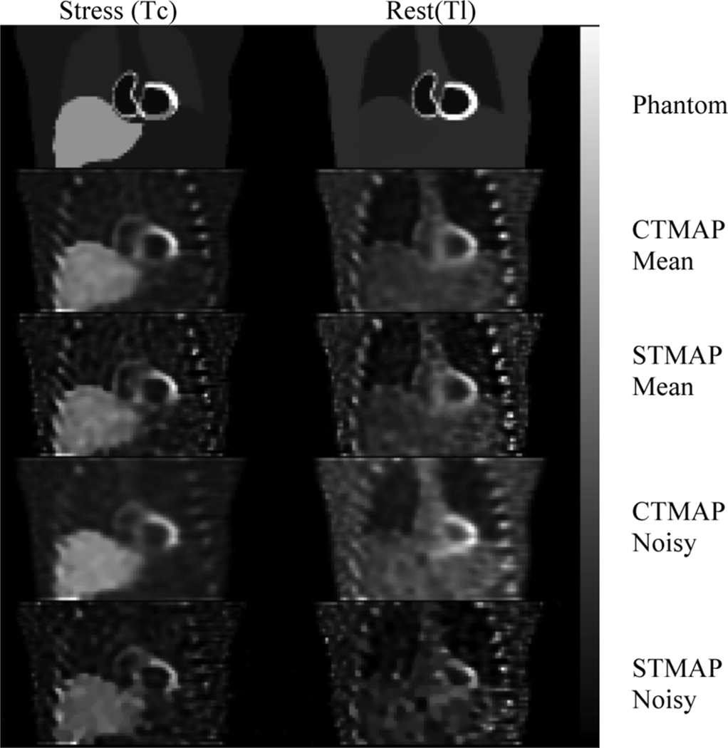
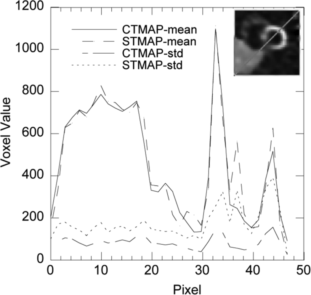
Fig. 6 shows coronal slices through the phantom, mean, and sample noisy images for both isotopes and both reconstruction algorithms. Note that the mean images contain some noise artifacts, partly because of the residual noise in the MC simulated data. From these images we see that edges corresponding to large activity discontinuities, such as at the boundary of the myocardium and chamber and liver and background, are sharp with both algorithms. Fig. 7 shows profiles through the mean images that illustrate the similar sharpness. In Fig. 6, the sample noisy images from CTMAP appear considerably less noisy inside uniform regions like the liver. This is further corroborated by the profile through the standard deviation image, shown in Fig. 7, where the standard deviation for CTMAP is on the order of 50% less than for STMAP.

Fig. 6.

Comparison of images reconstructed using the cross-tracer (CTMAP) and single-tracer (STMAP) algorithms. The rows are, top to bottom, the phantom, mean of 50 noisy CTMAP and STMAP reconstructions, and sample noisy CTMAP and STMAP reconstructions. The columns are (left to right) images of the rest and stress distributions. A 35% contrast myocardial perfusion defect was present in the stress distribution, but there was no defect in the rest distribution. All reconstructions were obtained using 16 subsets, 100 iterations, β = 0.05, and δ = 10.

Fig. 7.

Profiles through the mean stress image in Fig. 6 as well as standard deviation (std) images (not shown in Fig. 6) for the cross-tracer (CTMAP) and single-tracer (STMAP) algorithms at the position indicated in the inset image.

Also note that the images in Fig. 6 contain reversible defects, i.e., a defect-present in the stress image, and no defect in the rest image. Although the cross-tracer prior couples the smoothness on both images, the existence of a defect in the stress image did not induce a shadow in the rest image, as can be seen by comparing the mean rest images from CTMAP and STMAP in the defect region in the inferior wall of the left ventricle.

C. Effects of the Cross-Tracer Prior—Results From Fidelity Study

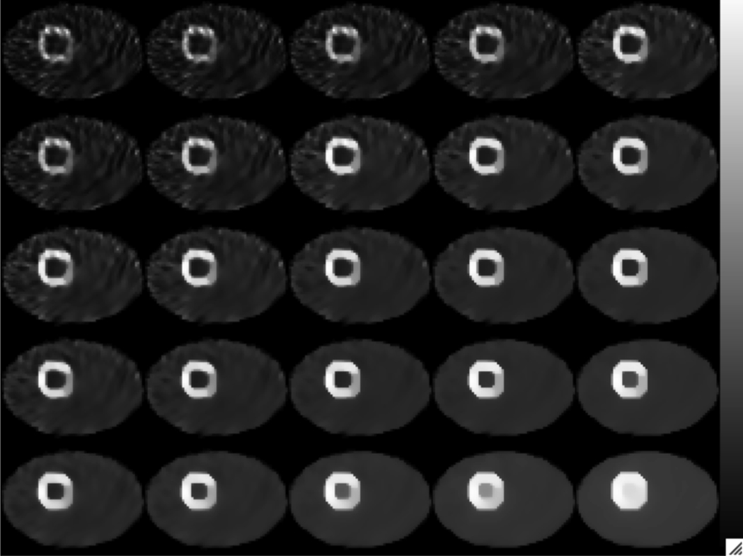
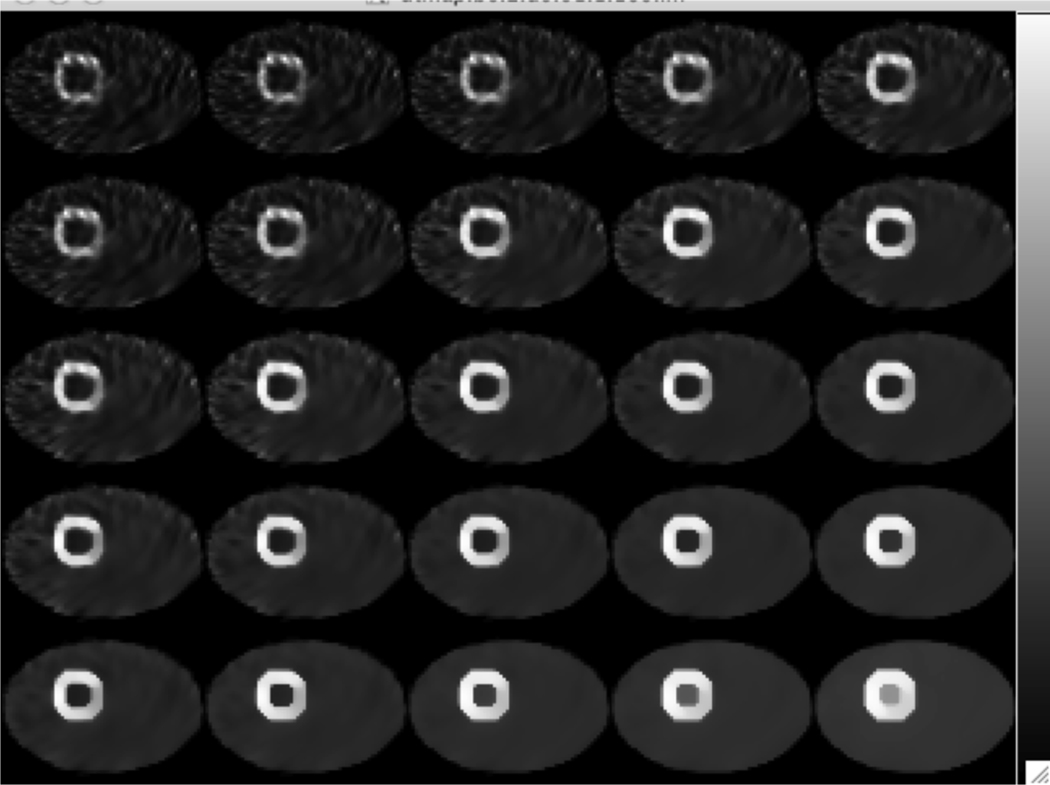
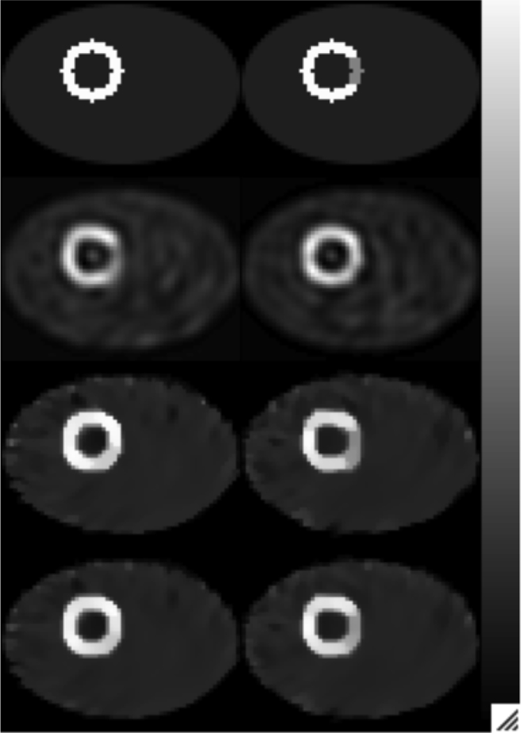
Figs. 8 and 9 show the slice containing the center of the heart reconstructed with STMAP and CTMAP, respectively, for a range of β and δ values. For the same values of β and δ, the cross-tracer reconstruction does a better job of preserving edges. This allows using a higher value of β, and thus increasing the smoothing in flat regions with the same edge preservation. For example, among all the combinations of β and δ, the one having the lowest MSE for CTMAP was β = 1.0 and δ = 0.1^−0.5, while for STMAP the best was β = 0.5, δ = 0.2^−0.5. Further, using these optimal combinations of priors, the MSE values for the stress and rest images were lower for CTMAP (stress 266.0, rest 275.0) than for STMAP (stress 297.2, rest 309.8). Both of these were substantially lower than the combination of OS-EM iteration and postreconstruction Butterworth filter cutoff frequency (five iterations and 0.20 pixel⁻¹) giving the lowest MSE (stress 406.3, rest 416.7). The rest and stress images for the optimal parameter values for each of the methods are shown, in comparison with the phantom images, in Fig. 10. Note in particular that the cross tracer prior did not induce shadow defects nor did it eliminate the real defect when appropriate values of the hyperparameters were used. These results indicate that, at least in terms of image fidelity, the MAP methods are better than OS-EM and, for the range of parameters investigated, the cross-tracer prior provides some advantage over a single-tracer prior having the same functional form.

Fig. 8.

Reconstructed stress images using STMAP (100 iterations, 16 subsets). The rows are for (top to bottom) β = 0.2, 0.5, 1.0, 2.0, and 5.0. The columns (left to right) are for δ^−1/2 = 0.01, 0.02, 0.05, 0.1, and 0.2.

Fig. 9.

Reconstructed stress images using CTMAP (35 iterations, 16 subsets). The rows are for (top to bottom) β = 0.2, 0.5, 1.0, 2.0, and 5.0. The columns (left to right) are for δ^−1/2 = 0.01, 0.02, 0.05, 0.1, and 0.2.

Fig. 10.

Optimal Images: Columns (left to right) rest and stress. Rows (top to bottom): true image; OS-EM (5 iterations, 16 subsets, cutoff = 0.2 pixel⁻¹); STMAP (β = 0.5, δ^−1/2 = 0.2) and CTMAP, (β = 1.0, δ^−1/2 = 0.1).

D. Three-Class Observer Study

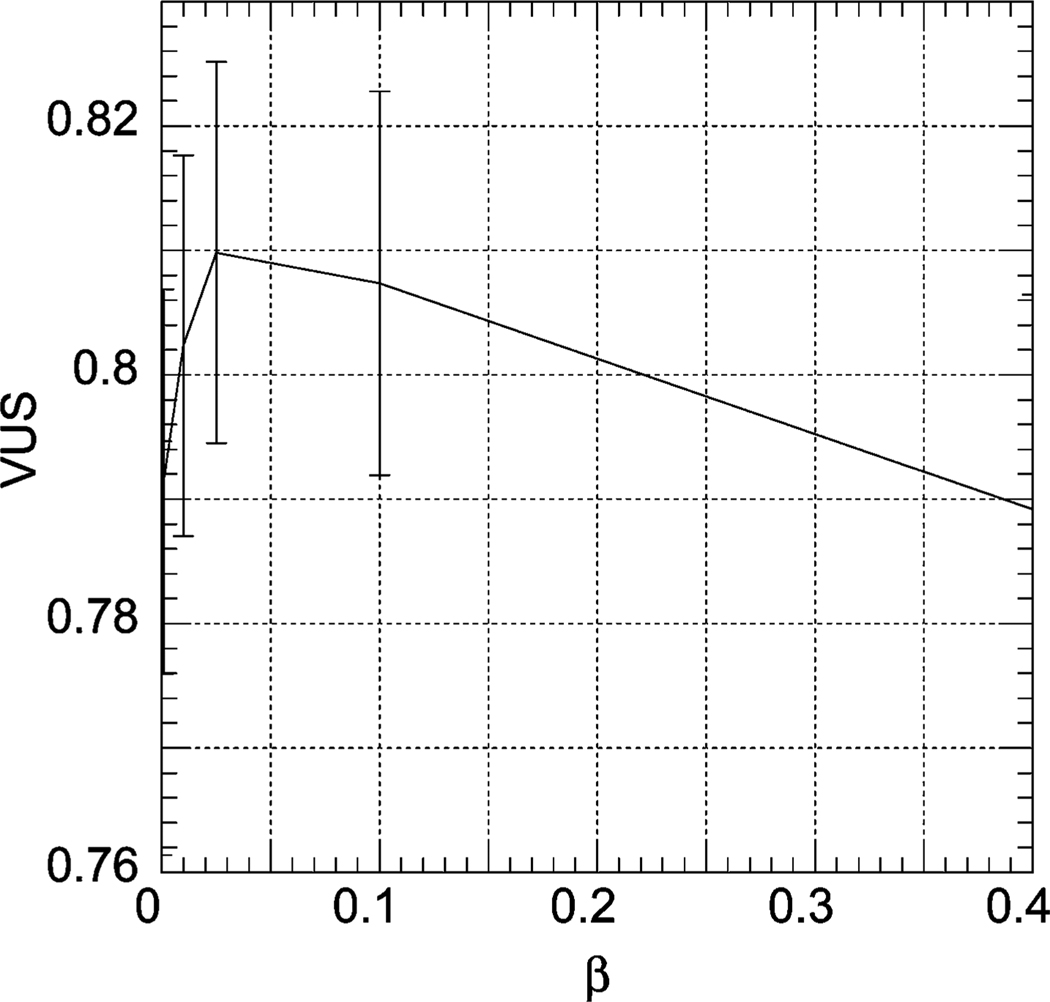
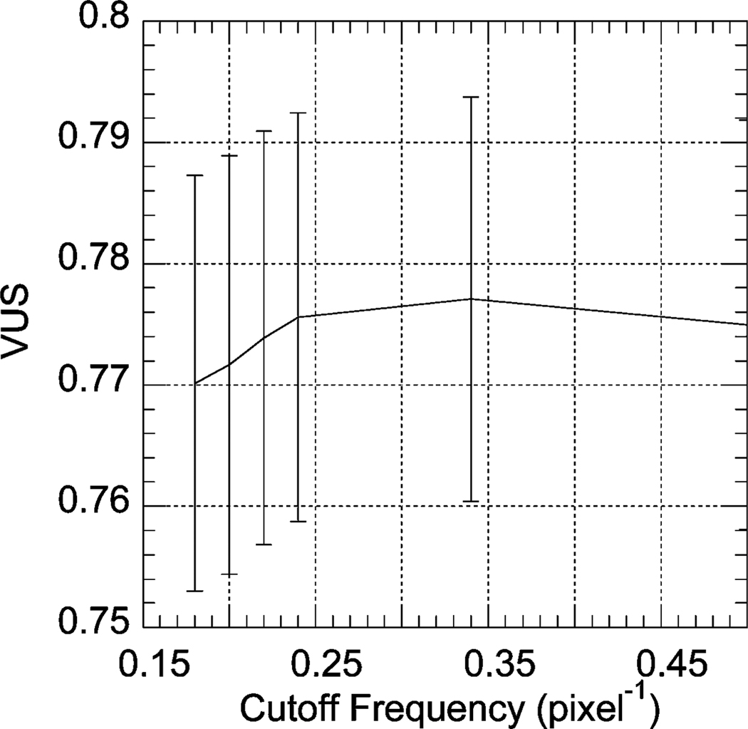
For cross-tracer MAP reconstruction, we used $\delta =\eta =\sqrt{2}$. These values were chosen based on qualitative evaluation of the image quality and were not formally optimized. We did, however, optimize the weight of the prior, β, by computing the value of the VUS for four different values of β in the range 0.001 to 0.4. The resulting VUS values are shown in Fig. 11. Fig. 12 shows the VUS values for OS-EM reconstruction with an order eight postreconstruction Butterworth filter as a function of the cutoff frequency. Table III shows a comparison of cross-tracer MAP and OS-EM with filtering using optimal parameters. It can be seen that cross-tracer MAP significantly improved the overall image quality as measured by the VUS. The p value for this difference using a two-tailed z-test was smaller than 0.001, indicating that this difference was highly statistically significant.

Fig. 11.

VUS values for cross-tracer MAP reconstruction.

Fig. 12.

VUS values for OS-EM reconstruction with postreconstruction Butterworth filtering.

TABLE III.

Comparison of Cross-Tracer MAP and OS-EM With Filtering Using Optimal Parameters

	VUS	Stddev
Cross-tracer MAP	0.818	0.015
OS-EM with filtering	0.761	0.016

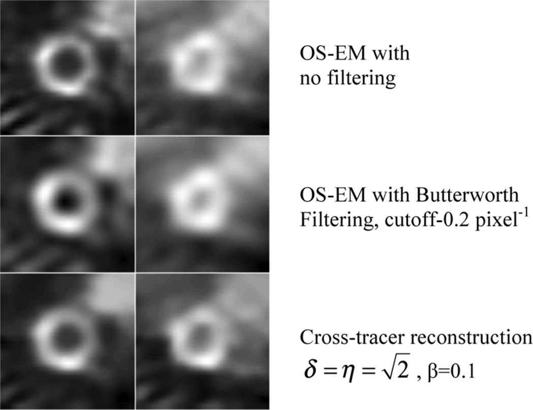
Fig. 13 shows some sample reconstructed images. The parameters for the reconstruction are also shown. It can be seen that the cross-tracer reconstruction improved the contrast in the ²⁰¹Tl image.

Fig. 13.

Sample reconstructed images. All images were obtained using seven iterations.

IV. Conclusion

In simultaneous dual isotope nuclear medicine imaging protocols, two or more images are simultaneously obtained from a patient to characterize different functional or anatomical features. The use of simultaneous acquisition means that these images are perfectly registered in space and time. To exploit commonalities in these images, we have proposed a cross-tracer prior that couples the voxel values in two perfectly registered images. We then developed convergent MAP algorithms, with and without ordered subsets acceleration, to optimize the resulting objective function. The algorithms were applied to dual-isotope MPS imaging using data that did not include crosstalk, and were compared to OS-EM with respect to its performance in a three-class diagnostic task. The addition of crosstalk and crosstalk compensation to the evaluation would have been desirable. However, crosstalk combined with crosstalk compensation would increase the noise of the ²⁰¹Tl images. Thus, one might hypothesize that this would increase the advantage of the cross-tracer prior. However, full evaluation of this remains a task for future work.

Results of both image resolution and noise and image fidelity studies showed that the proposed cross-tracer prior was superior to a single-tracer prior with the same functional form but without the cross-tracer coupling. Task-based evaluation studies showed that the proposed cross-tracer prior and the convergent algorithm substantially improved image quality for dual-isotope MPS images compared to OS-EM reconstruction with post-reconstruction filtering. In future work we will investigate more complete optimization of the hyperparameters of the cross-tracer prior and implementation of scatter and crosstalk compensation in the algorithm.

Appendix

Surrogate for the Cross-Tracer Prior: The cross-tracer prior, λ(x, y), is given by

$$\lambda (x,y)=\sqrt{1+{\left(\frac{x}{\delta }\right)}^2+{\left(\frac{y}{\eta }\right)}^2}-1.$$ (A1)

Define λ̅(x, y) as a quadratic function

$$\overline{\lambda }(x,y)=a+\frac{1}{2}{\mathit{\text{bx}}}^2+\frac{1}{2}{\mathit{\text{cy}}}^2$$ (A2)

with the coefficients a, b, and c to be determined such that

$$\{\begin{array}{c}\overline{\lambda }(x,y)\ge \lambda (x,y)\text{ for all the }x\hfill \\ \overline{\lambda }(x_0,y_0)=\lambda (x_0,y_0).\hfill \end{array}$$ (A3)

These conditions imply that λ̅ and λ have a common tangent at (x₀, y₀). Thus we obtain

$$\frac{d\overline{\lambda }(x,y)}{\mathit{\text{dx}}}{|}_{(x_0,y_0)}={\mathit{\text{bx}}}_0=\frac{d\lambda (x,y)}{\mathit{\text{dx}}}{|}_{(x_0,y_0)}={\lambda }_x^{\prime }(x_0,y_0)$$ (A4)

and

$$\frac{d\overline{\lambda }(x,y)}{\mathit{\text{dy}}}{|}_{(x_0,y_0)}={\mathit{\text{cy}}}_0=\frac{d\lambda (x,y)}{\mathit{\text{dy}}}{|}_{(x_0,y_0)}={\lambda }_y^{\prime }(x_0,y_0).$$ (A5)

Solving (A3), (A4) and (A5), for a, b, and c, and using the condition λ̅(x₀, y₀) = λ(x₀, y₀), we obtain

$$b=\frac{{\lambda }_x^{\prime }(x_0,y_0)}{x_0}$$ (A6)

$$c=\frac{{\lambda }_y^{\prime }(x_0,y_0)}{y_0}$$ (A7)

and

$$a=\lambda (x_0,y_0)-\frac{1}{2}{x}_0{\lambda }_x^{\prime }(x_0,y_0)-\frac{1}{2}{y}_0{\lambda }_y^{\prime }(x_0,y_0).$$ (A8)

Now we check the other condition in (A3), i.e., whether λ̅(x, y) ≥ λ(x, y), for all x and y. Denoting the difference of λ̅(x, y) and λ(x, y), as z(x, y), we see that

$$z(x,y)=\overline{\lambda }(x,y)-\lambda (x,y)=\lambda (x_0,y_0)-\frac{1}{2}{x}_0{\lambda }_x^{\prime }(x_0,y_0)-\frac{1}{2}{y}_0{\lambda }_y^{\prime }(x_0,y_0)+\frac{1}{2}\frac{{\lambda }_x^{\prime }(x_0,y_0)}{x_0}{x}^2+\frac{1}{2}\frac{{\lambda }_y^{\prime }(x_0,y_0)}{y_0}{y}^2-\lambda (x,y).$$ (A9)

Substituting (A1) into (A9), A.II provides a proof that z(x, y) achieves its minimum at (x₀, y₀). From (A6)–(A8), we see that λ̅(x, y) is

$$\overline{\lambda }(x,y)=[\lambda (x_0,y_0)-\frac{1}{2}{x}_0{\lambda }_x^{\prime }(x_0,y_0)-\frac{1}{2}{y}_0{\lambda }_y^{\prime }(x_0,y_0)]+\frac{1}{2}\frac{{\lambda }_x^{\prime }(x_0,y_0)}{x_0}{x}^2+\frac{1}{2}\frac{{\lambda }_y^{\prime }(x_0,y_0)}{y_0}{y}^2.$$ (A10)

We now define

$${\gamma }_y(x,y)=\frac{{\lambda }_y^{\prime }(x,y)}{y}\text{ and }{\gamma }_x(x,y)=\frac{{\lambda }_x^{\prime }(x,y)}{x}.$$ (A11)

Equation (A10) can thus be rewritten as

$$\begin{array}{cc}\overline{\lambda }(x,y)\hfill & =[\lambda (x_0,y_0)-\frac{1}{2}{x}_0{\lambda }_x^{\prime }(x_0,y_0)-\frac{1}{2}{y}_0{\lambda }_y^{\prime }(x_0,y_0)]+\frac{1}{2}{\gamma }_x(x_0,y_0)x^2+\frac{1}{2}{\gamma }_y(x_0,y_0)y^2\hfill \\ \hfill & =\frac{1}{2}{\gamma }_x(x_0,y_0)[x^2-2{\mathit{\text{xx}}}_0+x_0^2]+{\lambda }_x^{\prime }(x_0,y_0)x-\frac{1}{2}{\lambda }_x^{\prime }(x_0,y_0)x_0+\frac{1}{2}{\gamma }_y(x_0,y_0)[y^2-2{\mathit{\text{yy}}}_0+y_0^2]+{\lambda }_y^{\prime }(x_0,y_0)y-\frac{1}{2}{\lambda }_y^{\prime }(x_0,y_0)y_0+\lambda (x_0,y_0)-\frac{1}{2}{x}_0{\lambda }_x^{\prime }(x_0,y_0)-\frac{1}{2}{y}_0{\lambda }_y^{\prime }(x_0,y_0)\hfill \\ \hfill & =\frac{1}{2}{\gamma }_x(x_0,y_0){[x-x_0]}^2+\frac{1}{2}{\gamma }_y(x_0,y_0){[y-y_0]}^2+{\lambda }_x^{\prime }(x_0,y_0)(x-x_0)+{\lambda }_y^{\prime }(x_0,y_0)[y-y_0]+\lambda (x_0,y_0).\hfill \end{array}$$ (A12)

Now let

$$x=x_j-x_k\text{ and }y=y_j-y_k.$$ (A13)

Similarly,

$$x_0={\widehat{x}}_j-{\widehat{x}}_k\text{ and }{y}_0={\widehat{y}}_j-{\widehat{y}}_k.$$ (A14)

From the relationship

$${[x_j-x_k-({\widehat{x}}_j-{\widehat{x}}_k)]}^2={[\frac{1}{2}(2x_j-2{\widehat{x}}_j)+\frac{1}{2}(2{\widehat{x}}_k-2x_k)]}^2\le \frac{1}{2}{(2x_j-2{\widehat{x}}_j)}^2+\frac{1}{2}{(2x_k-2{\widehat{x}}_k)}^2$$ (A15)

we can find a surrogate function for λ̅(x_j − x_k, y_j − y_k; x̂_j − x̂_k, ŷ_j − ŷ_k), that is

$$\overline{\lambda }(x_j-x_k,y_j-y_k;{\widehat{x}}_j-x_k,y_j-y_k)\le {\lambda }_x^{\prime }({\widehat{x}}_j-{\widehat{x}}_k,y_j-y_k)[x_j-x_k-(x_j-x_k)]+{\lambda }_y^{\prime }({\widehat{x}}_j-{\widehat{x}}_k,y_j-y_k)[y_j-y_k-(y_j-y_k)]+\lambda ({\widehat{x}}_j-{\widehat{x}}_k,y_j-y_k)+\frac{1}{4}{\gamma }_x({\widehat{x}}_j-{\widehat{x}}_k,y_j-y_k)\times [{(2x_j-2x_j)}^2+{(2x_k-2x_k)}^2]+\frac{1}{4}{\gamma }_y({\widehat{x}}_j-{\widehat{x}}_k,y_j-y_k)\times [{(2y_j-2y_j)}^2+{(2y_k-2{\widehat{y}}_k)}^2].$$ (A16)

So, we now have a new surrogate function, ϕ(x_j, x_k, y_j, y_k), given by

$$\varphi (x_j,x_k,y_j,y_k)={\lambda }_x^{\prime }({\widehat{x}}_j-{\widehat{x}}_k,{\widehat{y}}_j-{\widehat{y}}_k)[x_j-x_k-({\widehat{x}}_j-{\widehat{x}}_k)]+{\lambda }_y^{\prime }({\widehat{x}}_j-{\widehat{x}}_k,{\widehat{y}}_j-{\widehat{y}}_k)[y_j-y_k-({\widehat{y}}_j-{\widehat{y}}_k)]+\lambda ({\widehat{x}}_j-{\widehat{x}}_k,{\widehat{y}}_j-{\widehat{y}}_k)+\frac{1}{4}{\gamma }_x({\widehat{x}}_j-{\widehat{x}}_k,{\widehat{y}}_j-{\widehat{y}}_k)\times [{(2x_j-2{\widehat{x}}_j)}^2+{(2x_k-2{\widehat{x}}_k)}^2]+\frac{1}{4}{\gamma }_y({\widehat{x}}_j-{\widehat{x}}_k,{\widehat{y}}_j-{\widehat{y}}_k)\times [{(2y_j-2{\widehat{y}}_j)}^2+{(2y_k-2{\widehat{y}}_k)}^2].$$ (A17)

Rearranging (A17), we obtain,

$$\varphi (x_j,x_k,y_j,y_k)={\gamma }_x({\widehat{x}}_j-{\widehat{x}}_k,{\widehat{y}}_j-{\widehat{y}}_k)\times \{{[x_j-\frac{1}{2}(x_j+x_k)]}^2+{[x_k-\frac{1}{2}(x_j+x_k)]}^2\}+{\gamma }_y({\widehat{x}}_j-{\widehat{x}}_k,y_j-y_k)\times \{{[y_j-\frac{1}{2}(y_j+y_k)]}^2+{[y_k-\frac{1}{2}(y_j+y_k)]}^2\}+C({\widehat{x}}_j-{\widehat{x}}_k,y_j-y_k)$$ (A18)

where

$$C({\widehat{x}}_j-{\widehat{x}}_k,{\widehat{y}}_j-{\widehat{y}}_k)=-{\gamma }_x({\widehat{x}}_j-{\widehat{x}}_k,{\widehat{y}}_j-{\widehat{y}}_k)\frac{1}{2}{({\widehat{x}}_j-{\widehat{x}}_k)}^2-{\gamma }_y({\widehat{x}}_j-{\widehat{x}}_k,{\widehat{y}}_j-{\widehat{y}}_k)\frac{1}{2}{({\widehat{y}}_j-{\widehat{y}}_k)}^2+\lambda ({\widehat{x}}_j-{\widehat{x}}_k,{\widehat{y}}_j-{\widehat{y}}_k)$$

is a constant that is independent of x_j, x_k, y_j, and y_k. Now we substitute (A18) into (4), and the surrogate function of the prior term is

$${\mathrm{\Lambda }}^{(n)}(\mathbf{x},\mathbf{y})=2{\displaystyle \sum _j^J}{\displaystyle \sum _{k\in N_j}}{\omega }_{\mathit{\text{jk}}}\{{\gamma }_x(x_j^{(n)}-x_k^{(n)},y_j^{(n)}-y_k^{(n)}){[x_j-\frac{1}{2}(x_j^{(n)}+x_k^{(n)}\left)\right]}^2\}+2{\displaystyle \sum _j^J}{\displaystyle \sum _{k\in N_j}}{\omega }_{\mathit{\text{jk}}}\{{\gamma }_y(x_j^{(n)}-x_k^{(n)},y_j^{(n)}-y_k^{(n)}){[y_j-\frac{1}{2}(y_j^{(n)}+y_j^{(n)}\left)\right]}^2\}+{\displaystyle \sum _j^J}{\displaystyle \sum _{k\in N_j}}{\omega }_{\mathit{\text{jk}}}C(x_j^{(n)}-x_k^{(n)},y_j^{(n)}-y_k^{(n)})$$ (A19)

where $C(x_j^{(n)}-x_k^{(n)},y_j^{(n)}-y_k^{(n)})$ is a constant that is independent of x and y. Note that in (A19) we used $x_j^{(n)}\text{ and }{y}_j^{(n)}$ to replace and x̂_j and x̂_j, respectively, for notational purposes. In particular, the superscript (n) denotes the estimate after the nth iteration. Simplifying Λ⁽ⁿ⁾ (x, y), we have

$${\mathrm{\Lambda }}^{(n)}(\mathbf{x},\mathbf{y})=2{\displaystyle \sum _{j=1}^J}{\displaystyle \sum _{k\in N_j}}{h}_{\mathit{\text{jk}}}^{(n)}(x_j)+2{\displaystyle \sum _{j=1}^J}{\displaystyle \sum _{k\in N_j}}{g}_{\mathit{\text{jk}}}^{(n)}(y_j)+C^{(n)}$$ (A20)

where

$$\begin{array}{c}{h}_{\mathit{\text{jk}}}^{(n)}(t)\triangleq {\omega }_{\mathit{\text{jk}}}{\gamma }_x(x_j^{(n)}-x_k^{(n)},y_j^{(n)}-y_k^{(n)})\times {[t-\frac{1}{2}(x_j^{(n)}+x_k^{(n)}\left)\right]}^2\hfill \\ g_{\mathit{\text{jk}}}^{(n)}(t)\triangleq {\omega }_{\mathit{\text{jk}}}{\gamma }_y(x_j^{(n)}-x_k^{(n)},y_j^{(n)}-y_k^{(n)})\times {[t-\frac{1}{2}(y_j^{(n)}+y_k^{(n)}\left)\right]}^2\hfill \end{array}$$

and C⁽ⁿ⁾ is a constant term that does not depend on x_j, x_k, y_j, and y_k.

z(x, y) in (A9) Achieves its Minimum at (x₀, Y₀): Substituting (A1) into (A9) and simplifying, z(x, y) becomes (A21), shown at the bottom of the page.

$$z(x,y)=\frac{2+{\left(\frac{x_0}{\delta }\right)}^2+{\left(\frac{y_0}{\eta }\right)}^2-2\sqrt{(1+{\left(\frac{x_0}{\delta }\right)}^2+{\left(\frac{y_0}{\eta }\right)}^2)(1+{\left(\frac{x}{\delta }\right)}^2+{\left(\frac{y}{\eta }\right)}^2)}}{2\sqrt{(1+{\left(\frac{x_0}{\delta }\right)}^2+{\left(\frac{y_0}{\eta }\right)}^2)}}$$ (A21)

In (A21), the denominator is greater than zero. Since $s=\sqrt{t}$ is a monotonically increasing function, proving the numerator is greater than zero is equivalent to proving that

$${[2+{\left(\frac{x_0}{\delta }\right)}^2+{\left(\frac{y_0}{\eta }\right)}^2]}^2\ge 4(1+{\left(\frac{x_0}{\delta }\right)}^2+{\left(\frac{y_0}{\eta }\right)}^2)(1+{\left(\frac{x}{\delta }\right)}^2+{\left(\frac{y}{\eta }\right)}^2)$$ (A22)

Simplifying (A22), we see that the inequality in (A22) is equivalent to

$${\left[\right({\left(\frac{x_0}{\delta }\right)}^2+{\left(\frac{y_0}{\eta }\right)}^2)-({\left(\frac{x}{\delta }\right)}^2+{\left(\frac{y}{\eta }\right)}^2\left)\right]}^2\ge 0.$$ (A23)

Since the left-hand side of (A23) is a quadratic function, it is true for any x and y, and thus the numerator of (A21) is greater than zero, and

$$z(x,y)\ge 0.$$ (A24)

References

- 1.Song X, Frey EC, Wang WT, Du Y, Tsui BMW. Validation and evaluation of model-based crosstalk compensation method in simultaneous Tc-99m stress and Tl-201 rest myocardial perfusion SPECT. IEEE Trans. Nucl. Sci. 2004 Feb.vol. 51(no. 1):72–79. [Google Scholar]
- 2.Wang WT, Frey EC, Tsui BMW, Tocharoenchai C, Baird WH. Parameterization of Pb X-ray contamination in simultaneous Tl-201 and Tc-99m dual-isotope imaging. IEEE Trans. Nucl. Sci. 2002 Jun.vol. 49(no. 3):680–692. [Google Scholar]
- 3.Kadrmas DJ, Frey EC, Tsui BMW. Simultaneous technetium-99m/thallium-201 SPECT imaging with model-based compensation for cross-contaminating effects. Phys. Med. Biol. 1999 Jul.vol. 44:1843–1860. doi: 10.1088/0031-9155/44/7/319. [DOI] [PMC free article] [PubMed] [Google Scholar]
- 4.He X, Song XY, Frey EC. Application of three-class ROC analysis to task-based image quality assessment of simultaneous dual-isotope myocardial perfusion SPECT (MPS) IEEE Trans. Med. Imag. 2008 Nov.vol. 27(no. 11):1556–1567. doi: 10.1109/TMI.2008.928921. [DOI] [PMC free article] [PubMed] [Google Scholar]
- 5.Hsiao I-T, Rangarajan A, Gindi GR. Provably convergent OSEM-like reconstruction algorithm for emission tomography. SPIE Med. Imag. 2002: Image Process. 2002:10–19. [Google Scholar]
- 6.De Pierro AR, Yamagishi MEB. Fast EM-like methods for maximum “a posteriori” estimates in emission tomography. IEEE Trans. Med. Imag. 2001 Apr.vol. 20(no. 4):280–288. doi: 10.1109/42.921477. [DOI] [PubMed] [Google Scholar]
- 7.De Pierro AR. A modified expectation maximization algorithm for penalized likelihood estimation in emission tomography. IEEE Trans. Med. Imag. 1995 Mar.vol. 14(no. 1):132–137. doi: 10.1109/42.370409. [DOI] [PubMed] [Google Scholar]
- 8.Ahn S, Fessler JA. Globally convergent image reconstruction for emission tomography using relaxed ordered subsets algorithms. IEEE Trans. Med. Imag. 2003 May;vol. 22(no. 5):613–626. doi: 10.1109/TMI.2003.812251. [DOI] [PubMed] [Google Scholar]
- 9.Lange K, Hunter DR, Yang I. Optimization transfer using surrogate objective functions. J. Computat. Graphical Stat. 2000;vol. 9:1–20. [Google Scholar]
- 10.Chang JH, Anderson JMM, Votaw JR. Regularized image reconstruction algorithms for positron emission tomography. IEEE Trans. Med. Imag. 2004 Sep.vol. 23(no. 9):1165–1175. doi: 10.1109/TMI.2004.831224. [DOI] [PubMed] [Google Scholar]
- 11.Browne J, De Pierro AR. A row-action alternative to the EM algorithm for maximizing likelihoods in emission tomography. IEEE Trans. Med. Imag. 1996 Oct.vol. 15(no. 5):687–699. doi: 10.1109/42.538946. [DOI] [PubMed] [Google Scholar]
- 12.Gunawardana A. Ph.D. dissertation. Baltimore, MD, USA: Dept. Electrical Computer Eng., Johns Hopkins Univ.; 2001. The information geometry of EM variants for speech and image processing. [Google Scholar]
- 13.Neal RM, Hinton GE. A view of the EM algorithm that justifies incremental, sparse, and other variants. In: Jordan MI, editor. Proceedings of the NATO Advanced Study Institute on Learning in Graphical Models. Norwell, MA: Kluwer Academic; 1998. pp. 355–368. [Google Scholar]
- 14.Hsiao IT, Rangarajan A, Gindi G. A new convergent map reconstruction algorithm for emission tomography using ordered subsets and separable surrogates. Proc. 2002 IEEE Int. Symp. Biomed. Imag. 2002:409–412. [Google Scholar]
- 15.Hsiao IT, Rangarajan A, Khurd P, Gindi G. An accelerated convergent ordered subsets algorithm for emission tomography. Phys. Med. Biol. 2004 Jun.vol. 49:2145–2156. doi: 10.1088/0031-9155/49/11/002. [DOI] [PubMed] [Google Scholar]
- 16.Hsiao IT, Khurd P, Rangarajan A, Gindi G. An overview of fast convergent ordered-subsets reconstruction methods for emission tomography based on the incremental EM algorithm. Nucl. Instrum. Methods Phys. Res. Section A-Accelerators Spectrometers Detectors Associated Equipment. 2006 Dec.vol. 569:429–433. doi: 10.1016/j.nima.2006.08.152. [DOI] [PMC free article] [PubMed] [Google Scholar]
- 17.Rangarajan A, Khurd P, Hsiao IT, Gindi G. Convergence proofs for COSEM-ML and COSEM-MAP algorithms. Tech. Rep. 2003 MIPL-03–1. [Google Scholar]
- 18.Erdogan H, Fessler JA. Joint estimation of attenuation and emission images from PET scans. IEEE Med. Imag. Conf. 2000:1672–1675. [Google Scholar]
- 19.De Pierro AR. On the relation between the ISRA and the EM algorithm for positron emission tomography. IEEE Trans. Med. Imag. 1993 Jun.vol. 12(no. 2):328–333. doi: 10.1109/42.232263. [DOI] [PubMed] [Google Scholar]
- 20.Gunawardana A, Byrne W. Convergence theorems for generalized alternating minimization procedures. J. Mach. Learn. Res. 2005;vol. 6:2049–2073. [Google Scholar]
- 21.Ahn S, Fessler JA, Blatt D, Hero AO. Convergent incremental optimization transfer algorithms: Application to tomography. IEEE Trans. Med. Imag. 2006 Mar.vol. 25(no. 3):283–296. doi: 10.1109/TMI.2005.862740. [DOI] [PubMed] [Google Scholar]
- 22.He X, Frey EC, Links JM, Gilland KL, Segars WP, Tsui BMW. A mathematical observer study for the evaluation and optimization of compensation methods for myocardial SPECT using a phantom population that realistically models patient variability. IEEE Trans. Nucl. Sci. 2004 Feb.vol. 51:218–224. [Google Scholar]
- 23.Segars WP, Tsui BM, Lalush DS, Frey EC, King MA, Manocha D. Development and application of the new dynamic nurbsbased Cardiac-Torso (NCAT) phantom. J. Nucl. Med. 2001 May;vol. 42:7p–7p. [Google Scholar]
- 24.Barclay AB, Eisner RL, DiBella EV. PET thorax model database. [Online]. Available: http://www.emory.edu/CRL/abb/thorax-model/Contents.html. [Google Scholar]
- 25.He X, Links JM, Gilland KL, Tsui BMW, Frey EC. Comparison of 180 degrees and 360 degrees acquisition for myocardial perfusion spect with compensation for attenuation, detector response, and scatter: Monte Carlo and mathematical observer results. J. Nucl. Cardiol. 2006 May-Jun;vol. 13:345–353. doi: 10.1016/j.nuclcard.2006.03.008. [DOI] [PubMed] [Google Scholar]
- 26.Song X, Segars WP, Du Y, Tsui BMW, Frey EC. Fast modelling of the collimator-detector response in Monte Carlo simulation of SPECT imaging using the angular response function. Phys. Med. Biol. 2005 Apr.vol. 50:1791–1804. doi: 10.1088/0031-9155/50/8/011. [DOI] [PubMed] [Google Scholar]