A Fast and Fully Automatic Method for Cerebrovascular Segmentation on Time-of-Flight (TOF) MRA Image

Abstract

The precise three-dimensional (3-D) segmentation of cerebral vessels from magnetic resonance angiography (MRA) images is essential for the detection of cerebrovascular diseases (e.g., occlusion, aneurysm). The complex 3-D structure of cerebral vessels and the low contrast of thin vessels in MRA images make precise segmentation difficult. We present a fast, fully automatic segmentation algorithm based on statistical model analysis and improved curve evolution for extracting the 3-D cerebral vessels from a time-of-flight (TOF) MRA dataset. Cerebral vessels and other tissue (brain tissue, CSF, and bone) in TOF MRA dataset are modeled by Gaussian distribution and combination of Rayleigh with several Gaussian distributions separately. The region distribution combined with gradient information is used in edge-strength of curve evolution as one novel mode. This edge-strength function is able to determine the boundary of thin vessels with low contrast around brain tissue accurately and robustly. Moreover, a fast level set method is developed to implement the curve evolution to assure high efficiency of the cerebrovascular segmentation. Quantitative comparisons with 10 sets of manual segmentation results showed that the average volume sensitivity, the average branch sensitivity, and average mean absolute distance error are 93.6%, 95.98%, and 0.333 mm, respectively. By applying the algorithm to 200 clinical datasets from three hospitals, it is demonstrated that the proposed algorithm can provide good quality segmentation capable of extracting a vessel with a one-voxel diameter in less than 2 min. Its accuracy and speed make this novel algorithm more suitable for a clinical computer-aided diagnosis system.

Introduction

A cerebrovascular accident (CVA) or stroke is a medical emergency resulting from an ischemia caused by thrombosis, stenosis, malformation, or a hemorrhage from a ruptured aneurysm. It can cause permanent neurological damage, complications, or death if not promptly diagnosed and treated. It is the second leading cause of death and the leading cause of adult disability in the world¹. Magnetic resonance angiography (MRA) is a type of magnetic resonance imaging (MRI) scan. It can provide volumetric pictures of the vasculature inside the body in the form of sequential cross-sectional images. To construct volume visualizations of the cerebral blood vessels from volumetric MRA images, the maximum intensity projection (MIP) technique^2,3 has been widely used by many clinicians. MIP is a volume rendering technique for 3-D data that selects the maximum voxel value along a line from the viewpoint to the plane of projection (2-D). MIP can clearly show the overall shapes and paths of the blood vessels and is computationally fast. However, its 2-D projections do not provide a good sense of depth for the volumetric data (e.g., the spatial relationship of overlapping vessels or the region of interest obscured by large bright structures). Three-dimensional (3-D) information about vascular connections, spatial positioning, and tubular shape changes are crucial for CVA diagnosis, quantitative analysis, and postoperative monitoring.

A variety of techniques for vascular segmentation from MRA have been proposed. These techniques can be divided into two general categories: skeleton based and non-skeleton based.⁴ The principle of skeleton-based techniques is the segmentation and reconstruction of vessels by first detecting the centerlines of the vessels from cross-sectional slices. The centerlines can be generated by vessel modeling methods. Several methods have been developed based on this principle.^5–9 On the other hand, non-skeleton-based techniques extract the vessels in 3-D directly.

Non-skeleton-based segmentation techniques have received considerable attention. Wilson et al.¹⁰, Chung et al.^11,12, El-Baz et al.^13,14, and Hassouna et al.¹⁵ proposed segmentation methods for cerebral vessels based on statistical models using an MRA dataset. The curve evolution theory and level set method have been applied to images to derive object boundaries. Yu et al.¹⁶, Farag et al.¹⁷, Yan et al.¹⁸, Deschamps et al.¹⁹, and Manniesing et al.²⁰ developed vessel segmentation methods based on geometric deformable models (level sets). Masutani et al.²¹ proposed the segmentation of vessel-like structures using mathematical morphology. In addition, some hybrid methods have been presented. Zana et al.²² combined morphology and curvature evaluation to segment vessel-like structures. Flasque et al.²³ proposed a method for the detection, representation, and visualization of a cerebral vascular tree using MRA images. The vascular tree is built by iteratively tracking the vessel centerlines using candidate voxels, which is achieved by intensity correction, diffusion filtering, and region growing. Passat et al.²⁴ introduced an atlas of the whole head to help to segment brain vessels from MRA images using a topology-preserving region-growing algorithm.

These existing vascular segmentation methods have at least one of the following limitations: (1) Gaussian distribution is generally assumed to express the probability distribution of the tissues in MRA images. However, this assumption is inconsistent with the truth and results in an error between the proposed model and the clinical data. (2) The maximum intensity gradient, as the only criterion, is frequently employed to determine vascular boundaries, but the gradient magnitudes are not sufficiently high in the boundaries of thin vessels with low contrast. (3) The regulation of parameters in geometric deformable models is difficult or not applicable which greatly influences the segmentation results. (4) User interactions are required to determine the seed region, or the starting and ending points of vessels. (5) The method is time consuming. (6) An evaluation with a limited number of datasets barely proves robustness of the algorithm.

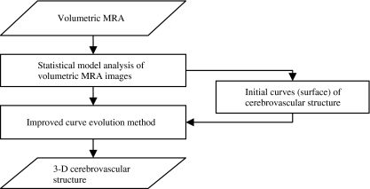
Therefore, the development of a fast and fully automatic cerebrovascular segmentation method that uses volumetric MRA data was the prime motivation behind our work. In this paper, we present an algorithm for segmenting a cerebrovascular tree from a time-of-flight (TOF) MRA dataset based on a statistical model analysis and curve evolution method. TOF MRA datasets was modeled by a finite mixture of one Rayleigh and several Gaussian distributions. Cerebral vessels distribution and other tissue (brain tissue, cerebrospinal fluid (CSF), and bone) distribution could be estimated using expectation maximization (EM) algorithm. Then the statistical distribution is integrated with gradient information to form a novel edge-strength for curve evolution. Such curve evolution method embedding the edge information is able to determine the boundary of vessels, particularly thin vessel, more accurately and robustly. Moreover, the curve evolution is implemented by a fast level set so as to able to segment the cerebrovascular structure in a short time. A flow chart for the algorithm is shown in Figure 1.

Fig. 1.

Flow chart for cerebrovascular segmentation of TOF MRA using statistical model and improved curve evolution.

Materials

The database used consisted of 200 TOF MRA studies from three different MRI scanners, including 142 normal cases and 58 abnormal cases (occlusions, unruptured aneurysm). (1) 110 of these MRA studies were performed using a GE Signa Series 1.5 T MRI scanner (TR = 29, TE = 6.9, flip angle = 20) at the Kizawa Hospital (KH), Japan. The volume was 256 × 256 × 80 voxels and the voxel size 0.47 × 0.47 × 1.5 mm³. (2) 70 of these MRA studies were obtained using a SIEMENS Symphony 1.5 T MRI scanner (TR = 44, TE = 7.15, flip angle = 20) at the Gero Hot Springs Hospital (GHSH), Japan. Each MRA study involved 72 slice images. The axial slice images were 256 × 192 pixels with a voxel size of 0.70 × 0.70 × 1 mm³. (3) The remaining 20 cases were acquired from a GE Signa Series 1.5 T MRI scanner (TR = 24, TE = 6.3, flip angle = 20) at Gifu University Hospital (GUH), Japan. The volume was 256 × 256 × 50 with a spatial resolution of 0.625 × 0.625 × 1.2 mm³. All of the acquired MRA data were subsequently converted to isotropic volume data by using tri-linear interpolation. The size of the converted 3-D volume data was 400 × 400 × 200 voxels, and the size of each voxel was 0.5 × 0.5 × 0.5 mm³. We tested our new segmentation method on the obtained isotropic volume dataset.

In addition, 10 sets of volumetric MRA images were selected from the database at random (five sets from KH, four sets from GHSH, one set from GUH), two of which are abnormal (one occlusions, one unruptured aneurysm). The cerebrovascular structures were manually segmented from these 10 datasets under the supervision of two experienced radiologists. The manual segmentations, which were voxel-by-voxel selections, were treated as the ground truth to determine segmentation precision and used for a statistical model analysis of blood vessels.

Statistical Model Analysis

In this section, we show how the statistical model for TOF MRA was derived for the various brain tissues in MRA images and estimate their parameters using the fast EM algorithm (FEM) algorithm.

Statistical Model

A statistical classification-based method of segmentation for medical images has been proposed²⁵. The basic idea behind this method is an assumption that the intensity of a homogeneous region (one anatomical structure) in an image submits to a single statistical model distribution and that the intensity distribution of all the pixels or voxels can be approximated by a finite mixture of statistical model distributions. A statistical model may also be a linear combination of several appropriate probability distribution functions based on the physical specialty of each anatomical structure in a specific imaging modality. It may automatically be determined whether a voxel is an object or background based on the statistical probability of the voxel. This method can be summarized as follows: (1) construct a statistical model with a finite mixture of probability distributions, (2) estimate the parameters for the statistical model, (3) obtain the probability distributions for the objects and background, respectively, and (4) select global threshold values based on the MAP classification rules.

A statistical approach-based cerebrovascular segmentation method using MRA images was first developed by Wilson and Noble.¹⁰ In their study, an intensity frequency histogram of a TOF MRA dataset had the property of an adjacent bimodal shape in a low-intensity region and a much lower frequency expansion over a high-intensity region. The lowest intensity region corresponded mainly to CSF (surrounding the brain tissue), bone, and the background air. The next lowest intensity region corresponded to brain tissues (both gray matter and white matter) and parts of the eyes. The highest intensity region consisted of subcutaneous fat and cerebral vessels. Two Gaussian distributions were chosen to model the bimodal shape in the lowest intensity regions respectively while a uniform distribution was used to depict the distribution of the vessels. El-Baz et al.¹⁴ adopted an adaptive linear combination of a derived model and a number of dominant and subordinate discrete Gaussians distributions rather than a mixture of just three pre-selected Gaussian and uniform distributions to approximate the intensity distribution of voxels in MRA datasets. In the study by Hassouna et al.¹⁵, one Rayleigh and two Gaussian distributions were used to model CSF and the brain tissue region. One Gaussian distribution corresponded to blood vessels. However, their statistical model for TOF MRA datasets was inadequate for our datasets. The above methods all rescaled the intensity values of the MRA voxels to the range [0,255] which results in the lost of detail information.

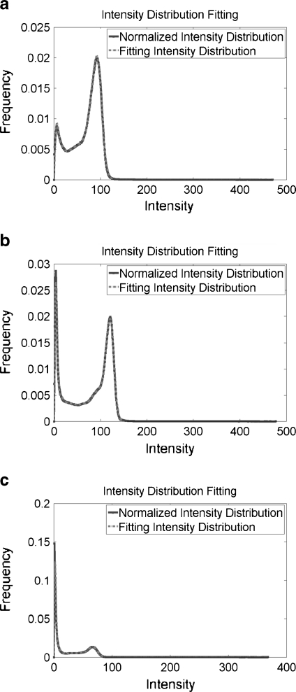
The intensity value of each voxel in our datasets was a 16-bit positive integer without any rescaling, ensuring accurate intensity information. The plots of the normalized intensity frequency histograms, without smoothing, of three TOF MRA datasets randomly selected from different MRI scanners are shown in Figure 2 (solid line). The normalized intensity frequency histograms for these three datasets have the same shape, two distinct peaks with a long tail over a high-intensity region. We need to construct a further general statistical model suitable for TOF MRA datasets from various MRI scanners.

Fig. 2.

The normalized intensity frequency histograms, without smoothing, of three TOF MRA datasets from a KH, b GHSH, c GUH, respectively (solid curve); and the fitting results by using the proposed statistical model (dashed curve).

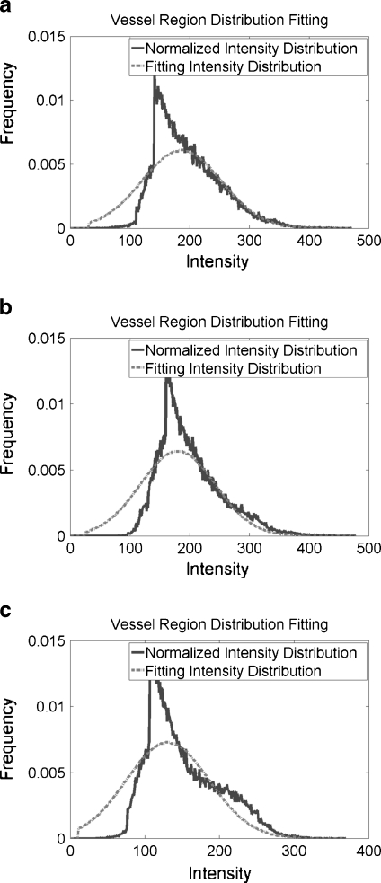
For cerebrovascular segmentation, blood vessels are the object while the background class includes CSF, bone, the background air, brain tissue, and parts of the eyes. The signal from blood vessels is dependent on flow rather than chemical structure in TOF MRA images. Blood vessels are generally regarded as circular vessels, and the intensity characteristics of the vessel voxels are assumed to exhibit a laminar flow pattern for which the vessel intensity is regarded as a uniform distribution.¹¹ This assumption, however, neglects blood viscosity, turbulence, and changes in the shape of vessels caused by cerebrovascular disease. The intractability of these factors makes it difficult to construct a single accurate statistical model for the intensity distribution of cerebral vessels in MRA images. To acquire a more reasonable statistical model for cerebral vessels, we considered the normalized intensity frequency histograms of 10 sets of manually segmented blood vessels from MRA in turn (see Fig. 3). The results predicted that a Gaussian class with large variance could be used to describe a statistical model of cerebral vessels in TOF MRA images.

Fig. 3.

Shows normalized intensity frequency histogram and the fitting results of vessel region from three datasets in Figure 2.

Rayleigh distribution provides a more accurate fit than Gaussian distribution for the lowest intensity region peak of a normalized intensity frequency histogram (peak1).¹⁵ The peak in the next lowest intensity region (peak2) can be expressed by a Gaussian distribution. The region between the first peak and second peak in a normalized intensity frequency histogram has an irregular shape, making it difficult to adopt a single probability distribution function to approximate that part of the observed histogram. A linear combination of several Gaussian distributions is able to deal with the problem by adjusting their mean and standard deviation.

The total probability density function for the intensity in TOF MRA images is expressed as follows,

1

where P_G() and P_G() denote Rayleigh and Gaussian distribution functions, respectively; is a parameter of a class k distribution function; denotes the parameter vector of the mixture model; is the prior probability vector. The Rayleigh distribution with parameter σ₀ and the Gaussian distributions with mean μ_k and standard deviation σ_k are given in Eqs. 2 and 3

2

3

Thus, Eq. 1 can be rewritten as

4

The parameters of these probability distributions can be estimated by using an expectation maximization algorithm.^26,27 It is well known that the EM algorithm is sensitive to the initialization of the parameter to be searched. Reasonable initialization of these parameters will guarantee iterations of EM to consistently converge to a local minimum that proves empirically value. An automatic method for parameter initialization can be referred (see Appendix). Besides, we adopted a fast EM algorithm²⁸ for reducing the computing time of EM algorithm.

Statistical Model Analysis

After obtaining the parameters for a statistical model of volumetric MRA data, we can derive the probability distributions for cerebral vessels and background, respectively.

According to the MAP classification, a voxel with intensity I_i will be classified as cerebral vessels if its posterior probability is greater than the background posterior probability

5

which can be rewritten as follows, based on Bayes rule and Eq. 2,

6

where P^*, μ^*, and σ^* are the final parameter estimations. The above equation means that a global threshold I_T for segmenting cerebral vessels from volumetric TOF MRA dataset can be obtained by calculating the intersection of the intensity distributions of the vessels and background.

Improved Curve Evolution

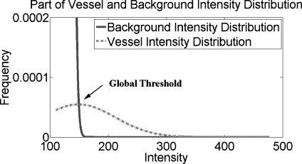
Experiments indicated that the global threshold segmentation method was able to entirely extract all of the main cerebrovascular structure, yet failed to segment the thin cerebral vessels with low contrast compared with neighboring tissues as the intensity distributions of those parts of the cerebral vessels were similar to those of brain tissue (gray matter and white matter; see the region within the circle in Fig. 4). This intensity similarity is caused by the small vessel diameter, slow flow velocity, and the turbulent flow in vessels.

Fig. 4.

A close-up of the intensity distributions of the cerebral vessels and background.

To deal with this under-segmentation, we next present an improved curve evolution method combined with region distribution obtained by statistical model analysis, gradient information, and spatial information (connectivity). First, we simply introduce the curve evolution and its applications in medical image segmentation. Then, we propose a novel evolution model based on region and edge information. Finally, a fast level set method is introduced to implement the curve evolution.

Curve Evolution and Its Application in Vessel Segmentation

Curve evolution, sometimes referred to as geometric curve evolution, has been applied to a wide variety of problems such as shape smoothing, shape recognition, and image segmentation.^29–32 One application of curve evolution in image segmentation is the well-known geometric active contours method. Malladi et al.³³ first proposed geometric active contours, which can be expressed by the following equation:

7

where g(I) is an edge-strength function, defined over the image domain, indicating the likelihood of an object boundary being present at any point in the image domain. C is the curve, and t is a time parameter. V₀ denotes a constant velocity, α is a positive coefficient, and K denotes the curvature of the curve. Let N be a normal vector to the curve. Generally, the edge-strength function is a continuous function, varying between 0 and 1 over the entire image domain. It equals or approaches the value 0 at the object boundaries and approaches the value 1 in homogeneous regions where the image gradient is small. Thus the geometric active contours method is a classical edge-based segmentation model.^34,35

Some region-based active contours methods^36–39 and active contours models that combine region and edge information^16,40,41 have been proposed to overcome the drawback of an edge-based model which is sensitive to the initial curve and noise. The curve evolution-based segmentation methods for 3-D vessels have previously been proposed.^16–20,42 Farag et al. proposed a 3-D cerebrovascular segmentation method using statistical model-based level sets from MRA. In their method, the segmentation model was a multi-objective minimization problem which used punishment terms (to preventing overlapping between regions), the clustering of homogeneous regions, and a smoothing term (shortening the length of the evolving curve). The trade-off among these three objectives makes the implementation of this model difficult. Yan et al. presented a capillary action model for extracting 3-D vessels from MRA data. A capillary active contour for the segmentation of thin vessels was derived. The selection of parameters is the big problem encountered with this the model. Furthermore, the results show that obvious thin vessels are not completely extracted from MRA datasets.

Region and Edge-Based Evolution Model for Vessel Segmentation

In Eq. 7, the sign of the velocity constant V₀ determines the direction of the curve evolution. When V₀ is positive, the curve expands; when negative, the curve contracts. Generally, the velocity of one point on the curve to be evolved is determined by the position of the point relative to the object to be segmented. If the point belongs to the object then the curve should locally extend; if it does not, the curve should contract. We performed this classification based on the statistical analysis results from the above section. A velocity function, rather than a velocity constant, based on Eq. 7 can thus be defined as:

8

If , the curve extends, otherwise the curve contracts. Notice that there is always . In our research, the initialization surfaces, obtained from the main cerebral vessels segmented on the basis of statistical analysis, need to be inflated to the boundary of the cerebral vessels under an external force. Thus, in the initial situation.

The external force is provided by the edge-strength function which incorporates the image properties, and is traditionally inversely proportional to the intensity gradient ∇I over the image domain. Such an edge-strength function will push the evolving curve to the high-gradient regions. However, gradient information has no meaning for low-contrast images and/or serious noise images (especially for medical images). Besides, a high gradient does not necessarily indicate a relevant boundary between the object and background. Especially for cerebral vessels in MRA images, they are widely distributed over the high-intensity region resulting in a heterogeneous intensity. There is a visible gradient magnitude in a location with marked changes in the flow velocity, caused by changes in the diameter of a vessel or cerebrovascular disease.

To overcome the single-factor limitation, region classification information is added into the edge-strength function. In most medical images, the segmentation threshold between different anatomical structures is in a dynamic region, which makes it impossible to use a global threshold to precisely segment the object from the background. The classification of pixels (voxels) outside of the dynamic region is precisely performed using region information. Inside of the dynamic region, the gradient information should be applied to distinguish the object from the background. Thus, we let the edge-strength function contain the region term and the gradient term . The dynamic region is given by , where I_T is a global threshold, and ∆ is the varying quantity of intensity, selected based on the special condition. The region term and the gradient term are defined respectively as:

9

10

where I_i denotes the intensity of the pixel (voxel) i. is the gradient of the smoothed version of the input image and p = 1 or 2. The Prewitt operator was adopted as a gradient operator in our research. The edge-strength function is defined as follows,

11

. Eq. 11 indicates that the region term predominates in the edge-strength function when the intensity is outside of the dynamic region; when it is not, the gradient term controls the edge-strength function. The new edge-strength function is still continuous over the entire intensity domain.

Another problem which we have to face to is how to evolve the curve along the vessel. The tip of the evolving curve along the stretch direction of vessel fails to further move forward due to the smooth action of curvature resulting in under-segmentation of thin cerebral vessel. We overcame the limitation by changing α in Eq. 7 from a positive constant coefficient to a positive variable. α should reduce curvature effect on smoothness when the point to be evolved is located near the centerline of vessel. Contrarily, if the point on the curve is close to the vessel boundary, the smooth action of curvature should be enhanced by increasing α. Therefore, Eq. 7 can be rewritten as

12

where α_i,j,k is a variable determined by vesselness^43–45.

Fast Level Set Method for Novel Evolution Model

The curve evolution model for segmentation is usually implemented with the aid of the level set method^46–48. Instead of explicitly representing a curve, the curve is implicitly embedded in a surface and all the level curves for the surface evolve simultaneously. The curve itself is the zero isosurface or zero level set. Level sets can develop sharp corners, break apart, and merge together, thus the topology changes in a curve can be handled automatically. The shortcoming of the level set method is that it is time consuming, especially for complex 3-D anatomical structure segmentation with a large volumetric size because all of the discrete points on the curve must be updated each time by approximating the spatial derivatives in the motion equations. All of the proposed cerebrovascular segmentation methods based on curve evolution^16–20 face this problem with time consumption ranging from 10 min to over hundreds of minutes. Nevertheless, fast cerebrovascular segmentation from an MRA dataset is crucial for a clinical computer-aided diagnosis (CAD) system. We therefore developed a fast level set method for new evolution model to expedite the segmentation process.

Construction of the level set function (i.e., signed distance function) is based on the level set method. Straightforward and intuitive level set function should simplify updating of level set function at every point in the image domain. Instead of adopting the standard distance function as level set function, we used an approximate level set function⁴⁹ as follows:

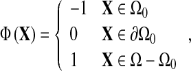13

where X is vector point in image. Let Ω denote the whole image domain, Ω₀ denotes object region, and ∂Ω denotes the boundary. That is, the level set functions at points inside and outside curve/surface are −1 and 1 separately, and the level set functions at points on the curve equal to 0.

The curve can be propagated by updating the level set function at a small set of points in the neighborhood of the zero level set (curve) instead of all the points in the image domain. Therefore, the updating of level set function is only performed at those grid points located in zero level set and their neighborhood points to be propagated to at next step (notice, not all of the neighborhood points of grid points) which reduces the computational labor to the dimension corresponding to the curve.

With approximate level set function, the points on the curve to be propagated will move one grid point along their velocity direction with one update. If the point moves outward, the value of level set function at it adds 1. Contrarily, the value of level set function at the point subtracts 1 when it contracts inward. This scheme simplifies computation of level set function, and does not require time step and reinitialization of level set function during the evolution, which are advantages of such scheme over traditional level set function.

We assume that every point on the curve would move to one of its neighborhood grid points along the velocity direction after one or several iterations. Which one first arrives at its neighborhood point depends on its velocity. The point with the fastest velocity on the moving curve would evolve to its neighborhood grid point earliest in the same time. We can therefore deduce if only one point on the updating curve will be evolved each iteration, the one with the fastest velocity would move to its neighborhood grid point at the following step. To speed up the evolution, the points with relatively faster velocity would evolve to their neighborhood grid points along their velocity direction each iteration, which can be expressed as the following,

14

where ε is a positive threshold value, numerical approximation of employs Upwind Finite Difference^46,47.

The curve evolution procedure stops if the following condition is satisfied.

15

As a summary, complete algorithm for fully automatic cerebrovascular segmentation using statistic model and improved curve evolution is described below.

Step 1: Calculate the probability distribution of the cerebral vessels and other brain tissue (background), and automatically obtain seed region of cerebral vessels

Step 2: Reconstruct main cerebrovascular structure using the region distribution obtained in Step 1

Step 3: Initialize the approximate level set function with surface of the main cerebrovascular structure using Eq. 13

Step 4: Compute edge-function g(Ii,j,k), velocity function V(Ii,j,k), restriction variable αi,j,k, and curvature K for the grid points on zero level set

Step 5: Iterate level set function based on Eq. 14

Step 6: If the stopping condition Eq. 15 is satisfied, stop; otherwise, go to Step 4

Results

The proposed 3-D vascular segmentation method, based on a statistical model and improved curve evolution, was applied to 200 TOF MRA datasets from three different MRI scanners, including the 10 MRA datasets used in the manual segmentation.

Statistical Model Results

In order to compare the goodness-of-fit of the estimating statistical model for the MRA dataset with the normalized intensity frequency histogram, the sum of absolute difference (SAD) was chosen to measure the similarity between them. SAD was defined as following:

16

where P_i is probability of intensity i, is estimating probability of intensity i. I_max is maximum value of intensity. We applied this statistical model, Wilson and Noble’ model²¹, and Hassouna’s model¹⁵ to 200 TOF MRA datasets from three different MRI scanners. The average SADs are listed in the Table 1. The comparison shows that average SADs using our model are obviously smaller than ones using other two models, which indicates that our statistical model is more applicable to TOF MRA from different MRI scanners. The difference of average SAD among the three sets of datasets is due to different imaging protocols.

Table 1.

Average SAD of three statistical models for TOF MRA datasets

Average SAD	Wilson Nobel model	Hassouna model	Our model
KH (110 datasets)	0.015	0.019	0.011
GHSH (70 datasets)	0.022	0.020	0.017
GUH (20 datasets)	0.020	0.019	0.016

The fitting results of three TOF MRA datasets from three different MRI scanners are shown in Figure 2. Solid line represents normalized intensity distribution and dotted line means fitting intensity distribution. Both lines show similar intensity distribution. Figure 3 especially shows the fitting results of vessel region from three datasets in Figure 2, in which solid line denotes the normalized intensity distribution of real MRA dataset and dashed line shows the fitting intensity distribution based on our proposed statistical model for TOF MRA. Because the intensity frequencies of cerebral vessels are far below those of the background region, a close-up of the intensity distributions for the cerebral vessels and background is shown in Figure 4. With the help of the automatic parameter initialization and FEM, parameter estimation for the statistical model of a TOF MRA dataset takes less than 3 s.

3-D Vascular Structure Segmentation Results

We used three metrics to quantify the differences between our proposed automatic segmentation and the manual segmentation over 10 datasets.

For binary segmentations, one approach for taking into account the spatial properties of structures is a pair-wise comparison of two binary segmentations by their relative volume overlap. Assuming spatial registration, the segmentation validation is analyzed voxel by voxel by using volume sensitivity defined as the intersection of the subject obtained by an automatic method and the reference (ground truth) in manual segmentation divided by the reference:

17

where denotes the set of all voxels in a dataset, ∩ is the intersection operator. S and R denote the subject and reference. The volume sensitivity gives a score of 1 for perfect agreement and 0 for complete disagreement. The volume sensitivities of the 10 datasets are shown in Table 2, and the average volume sensitivity over all 10 datasets is 93.6% with a standard deviation of 3.8%.

Table 2.

Validation of segmentation results for 10 datasets

		Edge-based active contours method			Proposed method
		VolSensitivity (%)	BranchSensitivity (%)	MADE (mm)	VolSensitivity (%)	BranchSensitivity (%)	MADE (mm)
KH	#1	83.6	90.4	0.563	98.0	100.0	0.227
	#2	82.3	90.4	0.416	96.2	98.1	0.164
	#3	85.9	92.3	0.631	97.1	98.1	0.302
	#4	81.6	88.5	0.747	95.7	96.2	0.478
	#5	81.3	90.4	0.730	96.8	98.1	0.102
GHSH	#6	70.7	84.0	1.198	90.5	96.0	0.541
	#7	71.6	86.0	0.813	89.3	96.0	0.435
	#8	68.7	82.0	1.407	87.5	92.0	0.397
	#9	77.9	90.0	0.812	88.9	92.0	0.386
GUH	#10	84.5	83.3	0.665	95.8	93.3	0.293
Mean±std		78.8 ± 5.9	87.73 ± 3.6	0.798 ± 0.28	93.6 ± 3.8	95.98 ± 2.8	0.333 ± 0.13

However, volume sensitivity has itself limitation because small vessels will have low contribution to it. Therefore branch sensitivity is brought forward here. It can be expressed by the following formula:

18

where denotes the number of all branches in extracted vascular structure. ∩ is the intersection operator. S and R denote the subject and reference, respectively. Evaluation standard of the branch sensitivity is same as volume sensitivity. 1 means perfect agreement and 0 represents complete disagreement. The branch sensitivities of the 10 datasets are also shown in Table 2. The average branch sensitivity over all 10 datasets is 95.98% with a standard deviation of 2.8%.

Another measure focus on distance error between each contour pairs in the automatic and manual segmentation. The segmentation validation is implemented by calculating mean distance error between two sets of true positive vessel contours (overlapped contours).⁵⁰ The comparison is performed in terms of contours on the 2D axial slices. To calculate the distance between two contours, generation method of distance function in the level set is employed. The vascular vessel boundaries (contours) on each axial slice obtained by automatic segmentation are regarded as zero level set. The distance function of the manual segmentation contour relative to zero level set is generated. The mean absolute distance error (MADE) therefore is calculated over all true positive contours in one dataset. It is expressed as follows,

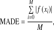19

where f(x_i) is distance function of discrete point x_i on manual segmentation contours, M is total number of discrete point on contours. The MADE are listed in Table 2 in terms of millimeters. The average of MADE over 10 datasets is about 0.333 mm.

For comparison, we also use the geometric active contours method³³ based on gradient information to extract cerebrovascular structure over 10 datasets, and calculate three metrics—volume sensitivity, branch sensitivity, and MADE. The results are reported in Table 2 too.

From the results of Table 2, the volume and branch sensitivity of segmentation results of the proposed method are greater than those of geometric active method based on gradient information for every case, while the MADE of segmentation results of the proposed method is smaller than one of geometric active method. The greater the sensitivity is and the smaller the MADE is, the higher the accuracy of the segmentation is. The results indicate that segmentation accuracy of the proposed method is obviously higher than one of the geometric active contours method only based on gradient information. In addition, branch sensitivity is obviously higher than volume sensitivity, which means that segmentation error of cerebral large vessel will greatly reduce the volume sensitivity of segmentation.

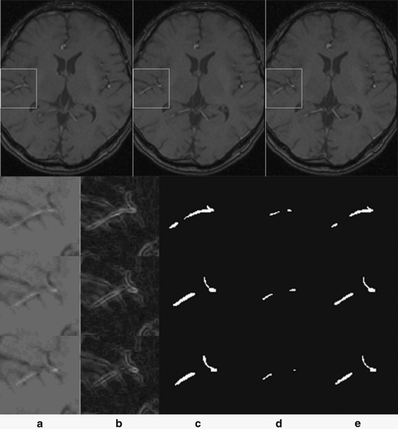
Figure 5 shows the segmentation results related to the region of interest (ROI) for three consecutive image slices, which is a piece of thin cerebral vessel which is difficult to segment. The first row gives three consecutive cross-sectional images, in which the ROI is enclosed by a rectangle. The following row corresponds to one ROI, in which column a shows the raw images for the ROI, column b gives the gradient images of the ROI obtained by using the Prewitt operator, column c shows the manual segmentations (i.e., the ground truth), column d gives the segmentation results using the general edge-based active contours method, and column e shows the segmentation results obtained by the proposed method. A comparison between columns a and b indicate that a high gradient does not necessarily indicate the boundary of a heterogeneous intensity object. The segmentation results in column d show that only vessels with a high flow velocity can be extracted using active contours based on general edge information while the end of the vessel could not be extracted. By comparing the automatic segmentation results using our method with the ground truth, it can be observed that the new segmentation method has a strong capacity for segmenting vessels with low contrast from a TOF MRA dataset.

Fig. 5.

Comparison of ROI for three consecutive image slices, (a) raw images, (b) gradient images, (c) manual segmentation, (d) edge-based active contours method, (e) proposed method results.

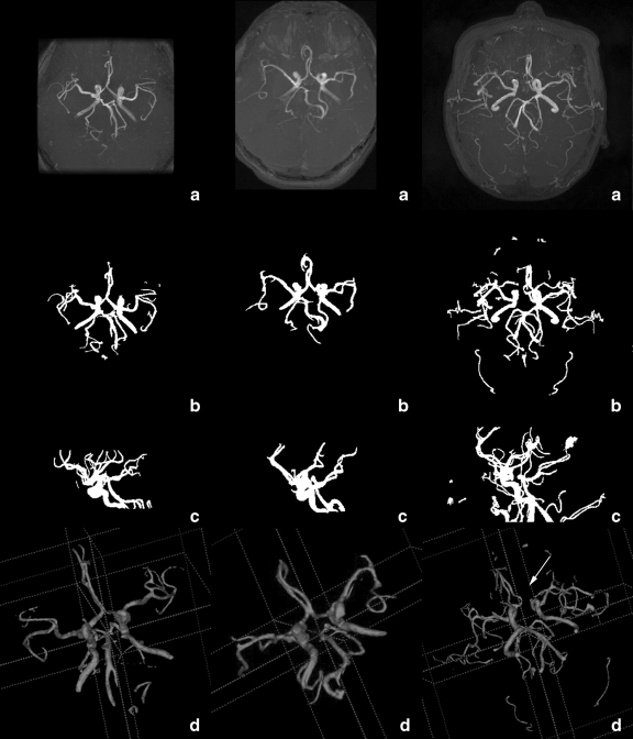
We evaluated the performance of the proposed segmentation method for 3-D cerebral structures by means of MIP images and 3-D rendered images of the segmented results. The 200 TOF MRA datasets from three different MRI scanners included 142 normal cases, 32 occlusion cases (21 cases from KH, eight cases from GHSH, and three cases from GUH), and 26 unruptured aneurysm cases (20 cases from KH, five cases from GHSH, and one case from GUH). An occlusion is marked by a loss in the route of the vessel. The occlusion cases could be more easily observed in the 3-D rendered images of the cerebrovascular segmentation results. The aneurysm is an abnormal bulging outward of one of the arteries in the brain. It is often difficult to directly detect the bulging by segmented results. Accurate cerebral vessel extraction, however, is crucial for computer-aided diagnosis of aneurysm. The 3-D renderings of the extracted cerebrovascular surfaces could be viewed stereoscopically, which is conducive to interpreting the spatial positions of vessels. Figure 6 shows three groups of volume visualizations for the segmented region, which are tabulated separately in different column. Each column is for one dataset. The MIP images of the raw TOF MRA dataset are shown in Row a. Rows b and c show the axial and sagittal MIP image of the segmented cerebral vessels, respectively. Row d is their 3-D rendered image. The discontinuity in the cerebral vessels caused by the occlusion, marked with an arrow, is easily observed. From comparisons among rows a, b, c, and d, we find that the segmentation results obtained by the proposed method were able to truly and intuitively depict the cerebrovascular structures and their spatial positions. The location of the occlusion can be more easily observed in the MIP images and 3-D rendering images of the segmentation results than in the raw MRA cross section images or their MIP images. This would be quite useful for the diagnosis of cerebral diseases, especially for use with a computer-aided diagnostic system. (3-D rendering images are acquired by using software ITK-Snap⁵¹).

Fig. 6.

Volume visualizations of the segmented region. Rows 1–3 are the KH, GHSH, and GUH datasets, respectively. a Axial MIP images of the raw dataset, b and c axial and sagittal MIP images of the segmentation results, d 3-D rendered images of the segmentation results. Illumination: arrow marks an abnormal broken vessel caused by occlusion.

Finally, from the perspective of objective representation of the cerebrovascular structure, the segmentation results were evaluated and given one of three grades by five different radiologists separately. Good case: over 90% of the vessels were extracted without obvious oversegmentation. Medium case: over 75% of the vessels were extracted, and a small quantity of oversegmentation was acceptable. Bad case: only the main vessels were extracted, or there was a large region of oversegmentation. The final average validation results are exhibited in Table 3, in which hospital datasets are represented separately. The good and medium grade occupancies of different hospitals are also given in Table 3.

Table 3.

Evaluation results from the clinical point of view

Case number	Good	Medium	Bad	Good and medium grade occupancy (%)
KH	87	22	1	99.1
GHSH	48	19	3	95.7
GUH	9	9	2	90.0
Total	144	50	6	97.0

The difference of good and medium grade occupancy among MRA datasets from three MRI scanners is due to difference of contrast between cerebrovascular region and surrounding tissue, influenced by imaging parameters.

The proposed method is computationally efficient. For a dataset with 400 × 400 × 200 voxels, the average time for segmenting a 3-D cerebrovascular structure was from 1 to 2 min on a 2.8 GHz PC with 2.0 GB RAM. 3-D vascular structure segmentation using level set deformable model generally can take as little as 10 min or up to several hours.^16–20

Discussion and Conclusion

In this paper, we have presented a fast, fully automatic segmentation algorithm for extracting a 3-D cerebrovascular structure from a TOF MRA dataset. It is a hybrid method, combining statistical model analysis with improved curve evolution. The cerebral vessels are modeled by one Gaussian distribution while other brain tissues are modeled by a finite mixture of one Rayleigh and several Gaussian distributions which are able to more precisely fit the TOF MRA dataset obtained under different imaging parameters. With distribution information of cerebral vessels and background, we presented an improved curve evolution method therefore, which constructs a novel edge-strength function employing the region distribution information of cerebral vessels and background obtained by above model analysis and gradient information together, capable of exacting thin cerebral vessels with similar intensity to brain tissue. Moreover, a fast level set method was developed to speed up implement of curve evolution.

In this work, the proposed algorithm was tested and evaluated using 200 clinical TOF MRA datasets from three different MRI scanners (different imaging parameters). Quantitative validations with ten sets of manual segmentation results showed that it had an average volume sensitivity of 93.6%, average branch sensitivity of 95.98%, and an average MADE of 0.333 mm. The comparisons of three metrics with geometric active contours method based on gradient information indicate that our proposed method has an obvious advantage in cerebrovascular segmentation, especially in thin vessel segmentation. Using the volume visualization technique, the 200 segmented cerebrovascular structures were then separately evaluated by five radiologists and given one of good, medium, and bad grades. The results indicated that the proposed method was able to provide a good quality of segmentation, especially for thin vessels with low contrast, and was capable of extracting vessels with a one-voxel diameter. The novel method was computationally efficient, taking on average 1–2 min to segment a 400 × 400 × 200 dataset. This makes time-critical medical applications possible, especially for computer-aided diagnosis.

Compared with other methods, the proposed automatic cerebrovascular segmentation method is far more superior in efficiency and generality for TOF MRA, which has been proven by a large number of clinical datasets. However, there are some limitations to the novel automatic segmentation method for cerebrovascular structure. In the proposed segmentation, image intensity was used as the only information either in the statistical analysis or in the curve evolution, resulting in leakages at areas where the image information is ambiguous. Hence, we conclude that image intensity is limited for complex cerebrovascular structure segmentation. In addition, curve evolution was locally determined. The information from derivatives of the curve, such as curvature, is too local to distinguish actual boundary from noise which frequently causes under-segmentation, for instance extraction failure of bulging outward. To overcome these limitations, we will combine shape model with the proposed curve evolution to segment tubular structures more robustly and accurately next step. The fully automatic cerebrovascular segmentation method is present for MRA of TOF mode. Further research is should be continued indicating whether the method is suitable for other mode MRA (e.g., phase-contrast MRA (PC MRA), contrast-enhanced MRA (CE MRA)), which are different in imaging signals.

In the future, we would like to obtain more manual segmentations for each dataset from different radiologists as the ground truth for quantitative evaluation. For quantitative segmentation validation, the overlap measure depends on the size and the shape complexity of the object, and is related to the image sampling. Thus, other quantitative evaluation methods⁴⁸ should be introduced in cerebrovascular segmentation validation. We will apply the segmented cerebrovascular structure in existing cerebrovascular disease CAD system.⁵² Finally, we plan to extend the technique to other medical image segmentation.

Appendix

Reasonable initialization of parameters will guarantee iterations of EM to consistently converge to a local minimum that proves empirically value. An automatic method for parameter initialization was developed. This initialization is based on the character of a normalized intensity histogram. The important procedure of the initialization is to estimate the parameters of the probability distributions corresponding to two distinct peaks with a long tail over a high-intensity region.

Let h(I) be the normalized intensity frequency corresponding to intensity I. The superscript 0 of the parameters presents initial value.

1. Peak1—Rayleigh distribution

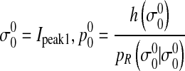σ₀ is parameter of Rayleigh distribution. P₀ is the prior probability of Rayleigh distribution.

1. Peak2—Gaussian distribution

, is calculated using the maximum likelihood estimation (MLE) for Gaussian distribution in the region

μ_n−1 and σ_n−1 are parameters of the Gaussian distribution. P_n−1 is the prior probability of the Gaussian distribution.

1. Long tail—Gaussian distribution

Find intensity I_vessel that satisfies 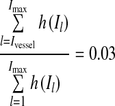. That is, we rudely estimate the threshold of vessels from the last 3% of the high-intensity data of the observed histogram.

. is calculated using the MLE ³¹ method for Gaussian distribution based on parameters , I_vessel and I_max. .

μ_n1 and σ_n are parameters of the Gaussian distribution relative to cerebral vessel. P_n is the prior probability of the Gaussian distribution.

The other Gaussian distributions equidistantly locate in the region

References

- 1."The top 10 causes of death," WHO, http://www.who.int/mediacentre/factsheets/fs310/en/index.html, 2002
- 2.Arlart IP, Bongartz GM, Marchal G. Magnetic Resonance Angiography. Tokyo: Springer; 1995. [Google Scholar]
- 3.Johnson DBS, Prince MR, Chenevert TL. Magnetic resonance angiography: A review. Academic Radiology. 1998;5(4):289–305. doi: 10.1016/S1076-6332(98)80230-4. [DOI] [PubMed] [Google Scholar]
- 4.Suri JS, Liu KC, Reden L, et al. A review on MR vascular image processing: Skeleton versus nonskeleton approaches: part II. Ieee Transactions on Information Technology in Biomedicine. 2002;6(4):338–350. doi: 10.1109/TITB.2002.804136. [DOI] [PubMed] [Google Scholar]
- 5.Wink O, Niessen WJ, Viergever MA. Fast delineation and visualization of vessels in 3-D angiographic images. Ieee Transactions on Medical Imaging. 2000;19(4):337–346. doi: 10.1109/42.848184. [DOI] [PubMed] [Google Scholar]
- 6.Krissian K, Malandain G, Ayache N, et al. Model-based detection of tubular structures in 3D images. Computer Vision and Image Understanding. 2000;80(2):130–171. doi: 10.1006/cviu.2000.0866. [DOI] [Google Scholar]
- 7.Yim PJ, Choyke PL, Summers RM. Gray-scale skeletonization of small vessels in magnetic resonance angiography. Ieee Transactions on Medical Imaging. 2000;19(6):568–576. doi: 10.1109/42.870662. [DOI] [PubMed] [Google Scholar]
- 8.Frangi AF, Niessen WJ, Hoogeveen RM, et al. Model-based quantitation of 3-D magnetic resonance angiographic images. Ieee Transactions on Medical Imaging. 1999;18(10):946–956. doi: 10.1109/42.811279. [DOI] [PubMed] [Google Scholar]
- 9.Aylward SR, Bullitt E. Initialization, noise, singularities, and scale in height ridge traversal for tubular object centerline extraction. Ieee Transactions on Medical Imaging. 2002;21(2):61–75. doi: 10.1109/42.993126. [DOI] [PubMed] [Google Scholar]
- 10.Wilson DL, Noble JA. An adaptive segmentation algorithm for time-of-flight MRA data. Ieee Transactions on Medical Imaging. 1999;18(10):938–945. doi: 10.1109/42.811277. [DOI] [PubMed] [Google Scholar]
- 11.Chung ACS, Noble JA. “Statistical 3D vessel segmentation using a Rician distribution”, Medical Image Computing and Computer-Assisted Intervention, Miccai'99. Proceedings. 1999;1679:82–89. [Google Scholar]
- 12.Chung ACS, Noble JA, Summers P. Fusing speed and phase information for vascular segmentation of phase contrast MR angiograms. Medical Image Analysis. 2002;6(2):109–128. doi: 10.1016/S1361-8415(02)00057-9. [DOI] [PubMed] [Google Scholar]
- 13.El-Baz A, Farag AA, Gimel'farb G, et al: “Automatic cerebrovascular segmentation by accurate probabilistic modeling of TOF-MRA images,” Medical Image Computing and Computer-Assisted Intervention—Miccai 2005, Pt 1, vol. 3749, pp. 34–42, 2005 [DOI] [PubMed]
- 14.El-Baz A, Farag AA, Gimel'farb G, et al: “A new adaptive probabilistic model of blood vessels for segmenting MRA images,” Medical Image Computing and Computer-Assisted Intervention—Miccai 2006, Pt 2, vol. 4191, pp. 799–806, 2006 [DOI] [PubMed]
- 15.Hassouna MS, Farag AA, Hushek S, et al. Cerebrovascular segmentation from TOF using stochastic models. Medical Image Analysis. 2006;10(1):2–18. doi: 10.1016/j.media.2004.11.009. [DOI] [PubMed] [Google Scholar]
- 16.Yu G, Li P, Miao Y, et al. Multiscale active contour model for vessel segmentation. Journal of Medical Engineering & Technology. 2008;32(1):1–9. doi: 10.1080/03091900600700798. [DOI] [PubMed] [Google Scholar]
- 17.Farag AA, Hassan H, Falk R, et al. 3D volume segmentation of MRA data sets using level sets—Image processing and display. Academic Radiology. 2004;11(4):419–435. doi: 10.1016/j.acra.2004.01.009. [DOI] [PubMed] [Google Scholar]
- 18.Yan P, Kassim AA. Segmentation of volumetric MRA images by using capillary active contour. Medical Image Analysis. 2006;10(3):317–329. doi: 10.1016/j.media.2005.12.002. [DOI] [PubMed] [Google Scholar]
- 19.Deschamps T, Schwartz P, Trebotich D et al: “Vessel segmentation and blood flow simulation using Level-Sets and embedded boundary methods,” in Conference of Computer Assisted Radiology and Surgery (CARS), Chicago, USA, pp. 75–80, 2004
- 20.Manniesing R, Velthuis BK, Leeuwen MS, et al. Level set based cerebral vasculature segmentation and diameter quantification in CT angiography. Medical Image Analysis. 2006;10(2):200–214. doi: 10.1016/j.media.2005.09.001. [DOI] [PubMed] [Google Scholar]
- 21.Masutani Y, Kurihara T, Suzuki M, et al. “Quantitative Vascular Shape Analysis for 3D MR-Angiography Using Mathematical Morphology”, in Conference of Computer Vision. Nice, France: Virtual Reality and Robotics in Medicine; 1995. pp. 449–454. [Google Scholar]
- 22.Zana F, Klein JC. Segmentation of vessel-like patterns using mathematical morphology and curvature evaluation. Ieee Transactions on Image Processing. 2001;10(7):1010–1019. doi: 10.1109/83.931095. [DOI] [PubMed] [Google Scholar]
- 23.Flasque N, Desvignes M, Constans JM, et al. Acquisition, segmentation and tracking of the cerebral vascular tree on 3D magnetic resonance angiography images. Medical Image Analysis. 2001;5(3):173–183. doi: 10.1016/S1361-8415(01)00038-X. [DOI] [PubMed] [Google Scholar]
- 24.Passat N, Ronse C, Baruthio J, et al. Region-growing segmentation of brain vessels: An atlas-based automatic approach. Journal of Magnetic Resonance Imaging. 2005;21(6):715–725. doi: 10.1002/jmri.20307. [DOI] [PubMed] [Google Scholar]
- 25.Wells WM, Grimson WEL, Kikinis R, et al. Adaptive segmentation of MRI data. Ieee Transactions on Medical Imaging. 1996;15(4):429–442. doi: 10.1109/42.511747. [DOI] [PubMed] [Google Scholar]
- 26.Dempster AP, Laird NM, Rubin DB. Maximum Likelihood from Incomplete Data Via Em Algorithm. Journal of the Royal Statistical Society Series B-Methodological. 1977;39(1):1–38. [Google Scholar]
- 27.Bilmes JA. A gentle tutorial of the EM algorithm and its application to parameter estimation for Gaussian mixture and hidden Markov models. Berkeley, California: International Computer Science Institute; 1998. [Google Scholar]
- 28.Patist JP. “A Fast Implementation of the EM Algorithm for Mixture of Multinomials”, in Conference of Advanced Data Mining and Applications. China: Xi'An; 2006. pp. 517–524. [Google Scholar]
- 29.Alvarez L, Guichard F, Lions PL, et al. Axioms and Fundamental Equations of Image-Processing. Archive for Rational Mechanics and Analysis. 1993;123(3):199–257. doi: 10.1007/BF00375127. [DOI] [Google Scholar]
- 30.Caselles V, Catte F, Coll T, et al. A Geometric Model for Active Contours in Image-Processing. Numerische Mathematik. 1993;66(1):1–31. doi: 10.1007/BF01385685. [DOI] [Google Scholar]
- 31.Shah J, “Shape recovery from noisy images by curve evolution,” in Conference on Signal and Image Processing, Las Vegas, U.S.A., 1995
- 32.Tsai A, Yezzi A, Willsky AS. Curve evolution implementation of the Mumford-Shah functional for image segmentation, denoising, interpolation, and magnification. Ieee Transactions on Image Processing. 2001;10(8):1169–1186. doi: 10.1109/83.935033. [DOI] [PubMed] [Google Scholar]
- 33.Malladi R, Sethian JA, Vemuri BC. Shape Modeling with Front Propagation—a Level Set Approach. Ieee Transactions on Pattern Analysis and Machine Intelligence. 1995;17(2):158–175. doi: 10.1109/34.368173. [DOI] [Google Scholar]
- 34.Caselles V, Kimmel R, Sapiro G. Geodesic active contours. International Journal of Computer Vision. 1997;22(1):61–79. doi: 10.1023/A:1007979827043. [DOI] [Google Scholar]
- 35.Siddiqi K, Lauziere YB, Tannenbaum A, et al. Area and length minimizing flows for shape segmentation. Ieee Transactions on Image Processing. 1998;7(3):433–443. doi: 10.1109/83.661193. [DOI] [PubMed] [Google Scholar]
- 36.Chakraborty A, Staib LH, Duncan JS. Deformable boundary finding in medical images by integrating gradient and region information. Ieee Transactions on Medical Imaging. 1996;15(6):859–870. doi: 10.1109/42.544503. [DOI] [PubMed] [Google Scholar]
- 37.Zhu SC, Yuille A. Region competition: Unifying snakes, region growing, and Bayes/MDL for multiband image segmentation. Ieee Transactions on Pattern Analysis and Machine Intelligence. 1996;18(9):884–900. doi: 10.1109/34.537343. [DOI] [Google Scholar]
- 38.Jones TN, Metaxas DN. “Image segmentation based on the integration of pixel affinity and deformable models”, in Conference on Computer Vision and Pattern Recognition (CVPR) USA: Santa Barbara; 1998. pp. 330–337. [Google Scholar]
- 39.Chesnaud C, Refregier P, Boulet V. Statistical region snake-based segmentation adapted to different physical noise models. Ieee Transactions on Pattern Analysis and Machine Intelligence. 1999;21(11):1145–1157. doi: 10.1109/34.809108. [DOI] [Google Scholar]
- 40.Mumford D, Shah J. Optimal Approximations by Piecewise Smooth Functions and Associated Variational-Problems. Communications on Pure and Applied Mathematics. 1989;42(5):577–685. doi: 10.1002/cpa.3160420503. [DOI] [Google Scholar]
- 41.Baillard C, Barillot C, Bouthemy P: Robust adaptive segmentation of 3D medical images with level sets, INRIA Technical Report, 2000
- 42.Descoteauxa M, Collinsb DL, Siddiqi K. A geometric flow for segmenting vasculature in proton-density weighted MRI. Medical Image Analysis. 2008;12(4):497–513. doi: 10.1016/j.media.2008.02.003. [DOI] [PubMed] [Google Scholar]
- 43.Frangi AF, Niessen WJ, Vincken KL et al: “Multiscale Vessel Enhancement Filtering ” in Conference on Medical Image Computing and Computer-Assisted Interventation (MICCAI), Cambridge, U.S.A., 1998, pp. 130–137
- 44.Cai WL, Dachille F, Harris GJ, et al. “Vesselness propagation: a fast interactive vessel segmentation method,” in Processings of the SPIE. San Diego, U.S.A: Medical Imaging; 2006. pp. 1343–1351. [Google Scholar]
- 45.Ye DH, Kwon DJ, Yun ID, et al: “Fast multiscale vessel enhancement filtering,” in Processings of the SPIE, Medical Imaging, San Diego, U.S.A, pp. 691423–691428, 2008
- 46.Sethian JA. Curvature and the Evolution of Fronts. Communications in Mathematical Physics. 1985;101(4):487–499. doi: 10.1007/BF01210742. [DOI] [Google Scholar]
- 47.Sethian JA. Level Set Methods and Fast Marching Methods: Evolving Interfaces in Computational Geometry, Fluid Mechanics, Computer Vision, and Materials Science. New York, U.S.A: Cambridge University Press; 1999. [Google Scholar]
- 48.Osher S, Fedkiw RP. Level set methods: An overview and some recent results. Journal of Computational Physics. 2001;169(2):463–502. doi: 10.1006/jcph.2000.6636. [DOI] [Google Scholar]
- 49.Lie J, Lysaker M, Tai XC. A binary level set model and some applications to Mumford-Shah image segmentation. Ieee Transactions on Image Processing. 2006;15(5):1171–1181. doi: 10.1109/TIP.2005.863956. [DOI] [PubMed] [Google Scholar]
- 50.Yang Y: “Image segmentation and shape analysis of blood vessels with applications to coronary atherosclerosis,” School of Biomedical Engineering, Georgia Institute of Technology, 2007
- 51.Yushkevich P, e. al: "itk-SNAP software," http://www.itksnap.org/pmwiki/pmwiki.php
- 52.Uchiyama Y, Gao X, Hara T, et al: “Computerized detection of unruptured aneurysms in MRA images: Reduction of false positives using anatomical location feature,” in SPIE Medical Imaging: Computer-aided diagnosis, San Diego, U.S., 2008, pp. 69151Q-1–69151Q-8