The Dynamical Response Properties of Neocortical Neurons to Temporally Modulated Noisy Inputs In Vitro

Abstract

Cortical neurons are often classified by current–frequency relationship. Such a static description is inadequate to interpret neuronal responses to time-varying stimuli. Theoretical studies suggested that single-cell dynamical response properties are necessary to interpret ensemble responses to fast input transients. Further, it was shown that input-noise linearizes and boosts the response bandwidth, and that the interplay between the barrage of noisy synaptic currents and the spike-initiation mechanisms determine the dynamical properties of the firing rate. To test these model predictions, we estimated the linear response properties of layer 5 pyramidal cells by injecting a superposition of a small-amplitude sinusoidal wave and a background noise. We characterized the evoked firing probability across many stimulation trials and a range of oscillation frequencies (1–1000 Hz), quantifying response amplitude and phase-shift while changing noise statistics. We found that neurons track unexpectedly fast transients, as their response amplitude has no attenuation up to 200 Hz. This cut-off frequency is higher than the limits set by passive membrane properties (∼50 Hz) and average firing rate (∼20 Hz) and is not affected by the rate of change of the input. Finally, above 200 Hz, the response amplitude decays as a power-law with an exponent that is independent of voltage fluctuations induced by the background noise.

Introduction

The response of a single neuron to a changing input is limited by the neuron's maximal spike frequency. Inputs which vary faster can only be encoded in the collective activity of a population. This can be observed in cortical rhythms when individual cells fire irregularly and at much lower spiking rate than the population rhythm revealed through local field potentials (Buzsaki and Draguhn 2004). Individual cells tend to fire more often at the peak of the oscillation but cannot emit a spike for every cycle. However, whereas 1 cell is in the refractory period another 1 may fire during the next cycle, so that the population can globally sustain fast rhythms. It is therefore of central importance to investigate how neurons respond to time-varying inputs and to identify the impact of synaptic background noise (Paré et al. 1998; Shadlen and Newsome 1998; Steriade 2001).

Previous theoretical studies (Knight 1972a; Gerstner 2000) extensively addressed these issues in models of spiking neurons. They emphasized the role of background noise in simplifying the neuronal response dynamics and allowing arbitrarily fast time-varying inputs to be encoded undistorted. Brunel et al. (2001) confirmed these theoretical findings for a more realistic mathematical description of synaptic background noise and quantitatively linked the temporal correlations of the background inputs (i.e., the synaptic filtering) to the response dynamics. However, by a more accurate description of the spike-initiation mechanisms in nonlinear integrate-and-fire neurons and conductance-based models, it was predicted that the linear response of a neuron is always dominated by a low-pass behavior, whose cut-off frequency is independent of the background noise as well as the rate of change of the input (Fourcaud-Trocmé et al. 2003; Fourcaud-Trocmé and Brunel 2005; Naundorf et al. 2005).

By investigating how the instantaneous firing rate is modulated by a noisy input with a small sinusoidal component, we experimentally estimated the linear response properties of layer 5 pyramidal cells of the rat somatosensory cortex, over a wide frequency range of input oscillations (i.e., 1–1000 Hz). We evaluated the extent of response linearity, tested the ability of cells to track temporally varying inputs, and investigated the impact of background noise. In the limit of small input amplitude, this allows one to predict the spiking activity of a population of weakly interacting neurons, on the basis of the single-cell responses to elementary sinusoidally modulated currents. This also allows to study how neurons take part in collective rhythms, inferring the preferred global frequency in recurrent networks (Fuhrmann et al. 2002; Brunel and Wang 2003; Wang 2003; Geisler et al. 2005) where each cell responds to a correlated foreground rhythm (i.e., the signal) while experiencing a distinct synaptic background activity.

Although the response properties of cortical neurons to stationary fluctuating inputs have been previously characterized (Chance et al. 2002; Rauch et al. 2003; Giugliano et al. 2004; Higgs et al. 2006; La Camera et al. 2006; Arsiero et al. 2007), this is the 1st time that the response of cortical neurons to temporally modulated inputs is investigated over a wide range of input frequencies and through analysis of the background noise.

Materials and Methods

Experimental Preparation and Recordings

Tissue preparation was as described in Rauch et al. (2003). Briefly, neocortical slices (sagittal, 300 μm thick) were prepared from 14- to 52-days-old Wistar rats. Large layer 5 (L5), regular-spiking pyramidal cells (McCormick et al. 1985) of the somatosensory cortex with a thick apical dendrite were visualized by differential interference contrast microscopy. Some neurons were filled with biocytin and stained (Hsu et al. 1981), to check that the entire neuronal apical dendrite was indeed in the plane of the slice, which was always the case. Whole-cell patch-clamp recordings were made at 32 °C from the soma (10–20 MΩ access resistance) with extracellular solution containing (in mM): 125 NaCl, 25 NaHCO₃, 2.5 KCl, 1.25 NaH₂PO₄, 2 CaCl₂, 1 MgCl₂, 25 glucose, bubbled with 95% O₂, 5% CO₂, perfused at a minimal rate of 1 mL/min. Electrode resistance and capacitance were 6.97 ± 0.18 MΩ and 23.73 ± 1.11 pF, respectively, when filled with an intracellular solution containing (in mM): 115 K-gluconate, 20 KCl, 10 4-(2-hydroxyethyl)-1-piperazineethanesulfonic acid (HEPES), 4 adenosine triphosphate-Mg, 0.3 Na₂-guanosine triphosphate, 10 Na₂-phosphocreatine, pH adjusted to 7.3 with KOH. All the chemicals were from Sigma or Merck (Switzerland). Other pipette solutions were reported not to alter significantly the response properties of the cells under very similar experimental conditions (Rauch et al. 2003). A BVC-700A bridge amplifier (Dagan Corporation, MN) was used in current-clamp mode and bridge balance and capacitance neutralization were routinely applied. Hyperpolarizing current steps and linear swept sine waves (ZAP) were injected to obtain estimates of the passive properties of patched neurons, such as the total membrane capacitance C_m and apparent input resistance R_in (Iansek and Redman 1973), as well as the membrane impedance amplitude profile (Hutcheon et al. 1996). Signals were low-pass filtered at 2.5 kHz, sampled at 5–15 kHz, and captured on the computer.

Finally, care was taken to ensure that the neuronal response was consistent and reproducible throughout the whole recording session (see Fig. 1b). The total whole-cell resistance R_in and the resting membrane voltage E_m were continuously monitored (during T₂ and T₁, respectively, located as in Fig. 1). Data collection began after these observables attained stable values and the experiment was stopped in case of any drift.

Figure 1.

In vivo–like stimulation protocol and the stability of in vitro recording conditions. In vivo irregular background synaptic inputs were emulated in vitro by injection of noisy currents under current-clamp. Specifically, gaussian currents characterized by mean I₀, standard deviation s and correlation time τ, were injected into the soma of layer 5 pyramidal cells. A deterministic sinusoidally oscillating waveform of amplitude I₁ and modulation frequency f was then superimposed to the background noise (a—lower trace), and the stimulation trials were interleaved by a recovery interval T_rec. The initial segments of each stimulus (i.e., lasting T₁, T₂, and T₃) were used to monitor the stability of the recording conditions on a trial-by-trial basis. Panel b shows a typical experimental session, plotting over time the whole-cell resistance R_in (estimated during T₂, b—upper panel), the resting membrane potential E_m (averaged during T₁, b—middle panel), as well as the reproducibility of the cell discharge rate r_fix, evaluated in response to a stationary noise, characterized by fixed statistics (s, τ)_fix (during T₃). Continuous lines in (b) represent average values of each observable across the whole experiment, whereas the gray shading in (b—lower panel) indicates a confidence level of approximately 68%, which describes the variance allowed for the data. The middle panel shows a layer V pyramidal cell of the somatosensory cortex of the rat stained with Biocytin.

The results reported here represent data from L5 pyramidal cells (n = 67) of the somatosensory cortex. The average resting membrane potential was E_m = −66 ± 4.4 mV, the apparent input resistance (R_in) was 45 ± 2.6 MΩ, the membrane time-constant (τ_m) was 18.32 ± 0.8 ms. The total capacitance C_m was estimated as 448 ± 19 pF. Liquid junction potentials were left uncorrected.

Injection of Sinusoidal Noisy Currents

To probe the response dynamics of pyramidal cells under in vivo–like conditions, independent realizations of a noisy current were computer-synthesized and injected somatically in current-clamp configuration (see Fig. 1a). Each experiment consisted of the repeated injection of current stimuli I(t), lasting T = 10–30 s each, interleaved by a recovery T_rec of 30 s. A deterministic sinusoidally oscillating current with frequency f was superimposed to the noisy current component and injected (Fig. 2c,d), so that

(1)

I_noise(t)was generated as a realization of an Ornstein–Uhlenbeck stochastic process with zero-mean and variance s² (Rauch et al. 2003), and independently synthesized for each repetition by iterating the equation

(2)

where ξ_t represents a random variable from a normal distribution (Press et al. 1992), and it was updated at every time step dt (i.e. 5–15 kHz). I_noise(t) is then an exponentially filtered white-noise and it aims at mimicking in vitro the barrage of a large numbers of balanced background excitatory and inhibitory synaptic inputs at the soma (Destexhe et al. 2001, 2003; Rauch et al. 2003; Arsiero et al. 2007). I_noise(t) is characterized by a steady-state Gaussian amplitude-distribution with zero-mean and variance s², and by a steady-state autocorrelation function exponentially decaying with time constant τ. The value of τ corresponds to the decay time-constants of individual synaptic currents and it was varied in the range 5–100 ms, thereby referring to fast (AMPA- and GABA_A-mediated) as well as slow (NMDA- and GABA_B-mediated) synaptic currents (Tuckwell 1988; Rauch et al. 2003). The choice of s² was aimed at mimicking the membrane voltage fluctuations observed in cortical recordings in vivo, which are around 3–5 mV (Paré et al. 1998), and it is also effectively representative of nonzero cross-correlations of background inputs (Rudolph and Destexhe 2004).

Figure 2.

Analyzing the discharge response to the oscillatory input signal over a background of irregular synaptic inputs. Irregular spike trains were evoked in the same neuron by sinusoidally modulated noisy current injections. The time of occurrence of each action potential (a, b) was referred to its peak and represented by a thick vertical mark. Lower panels show the spike raster-plots collected for different input modulation frequencies, f = 10 Hz and f = 250 Hz. The instantaneous firing rate r(t) (c, d—upper panels) reveals a sinusoidal modulation in time. This was estimated by the peristimulus time histograms (PSTHs) (bars) across repeated trials and successive input cycles, and quantified by the best-fit sinusoid with frequency f (black thick line). For the sake of comparison, the sinusoidal component of I(t) (c, d—lower panels) was plotted in red and superimposed to the actual injected waveform. Although the mean firing rate r₀ remains constant, its modulation r₁ and phase-shift Φ depend on the input frequency f.

The number of repetitions for the same set of stimulation parameters (I₀, I₁, s, τ, f) was 5–20, approximately ensuring an accuracy of at least 10% on the estimate of the instantaneous firing rate, with a confidence of 68% (see Rauch et al. 2003). Waveforms were injected in a random order to minimize the effect of slow drifts in the recording conditions. Although the explored range for f was 1–1000 Hz, the effect of distinct values for τ and for (I₀, s) was also investigated (as in Figs 5 and 6). Stimulations by a single sinusoid at the time were preferred to probing simultaneously the entire frequency-domain, with the aim of shortening each stimulation epoch in favor of the stability of the recordings (Fig. 1) and of the signal-to-noise ratio.

Figure 5.

The intensity of background fluctuations affects the dynamical response of cortical neurons. The impact of the noise variance s² was examined across a wide range of input frequencies f, in 4 distinct cells (a–d), under the same conditions of Figure 3. Strong background noise smoothes r₁(f) at intermediate frequencies, as in a programmable equalizer. Linear instead of logarithmic scale has been employed here for the y-axis. Each subpanel (top to bottom) reports r₁(f) and Φ(f), identifying the suprathreshold or weak-noise regime (“supra”—black markers) and the subthreshold or strong-noise regime (“sub”—red markers) by different marker shapes and colors. Each regime is characterized by distinct values for I₀ and s², adapted to yield a similar mean rate r₀ ∼ 20 Hz. Experimental data points (markers) have been plotted together with the best-fit predictions from a phenomenological filter model (continuous traces). For these cells, band-pass 2nd-order filters (i.e., n = 2—eq. 6) were found to describe the experimental data with high significance (see Supplemental Table S1). Error bars represent the 95% confidence intervals, obtained by the Levenberg–Marquardt fit algorithm. High-frequency error bars were large because of the poor signal-to-noise ration as well as for the ambiguity of the (periodic) estimates of Φ(f). Although I₁ = 50 pA and τ = 5 ms were fixed for all cells and both regimes, the remaining stimulation parameters were: (suprathreshold) (I₀, s)_a = (500, 50), (I₀, s)_b = (400, 20), (I₀, s)_c = (250, 25) and (I₀, s)_d = (350, 50) pA; (subthreshold) (I₀, s)_a = (300, 400), (I₀, s)_b = (150, 325), (I₀, s)_c = (100, 250) and (I₀, s)_d = (100, 450) pA.

Figure 6.

The timescale of background fluctuations affects the dynamical response of cortical neurons. The effect of the timescale of fluctuations (i.e., correlation time τ) was examined across a wide range of input frequencies f, in 4 cells (a–d). At high input frequencies pyramidal neurons are insensitive to the noise-color, in the sense that they do not speed up or slow down their fastest reaction time, for “white” or “colored” background noise. Linear instead of logarithmic scale has been employed here for the y-axis. The panels (top to bottom) report r₁(f) and Φ(f), with different marker shapes and colors referring to 2 stimulation regimes, indicated as τ_slow (red markers) and τ_fast (black markers). Although τ_fast was fixed to 5 ms and τ_slow was (a–d) 45–50 ms, in (d) the range 5–100 ms could be explored. As in Figure 5, experimental data points (markers) have been plotted together with the best-fit predictions from a phenomenological filter model (continuous and dashed traces). For these cells, band-pass third-order filters (i.e., n = 3—eq. 6) were found to describe the data with high significance (see Supplemental Table S2). Error bars represent the 95% confidence intervals obtained by the Levenberg–Marquardt fit algorithm. High-frequency error bars were large because of the poor signal-to-noise ration as well as for the ambiguity of the (periodic) estimates of Φ(f). Stimulation parameters were: (I₀, I₁, s)_a = (250, 50, 100), (I₀, I₁, s)_b = (300, 50, 100), (I₀, I₁, s)_c = (300, 50, 100), and (I₀, I₁, s)_d = (300, 50, 75) pA.

Injection of Noisy Broadband Waveforms

We also injected periodic broadband waveforms instead of sinusoids, under background noise I_noise(t). In analogy to equation (1), the stimulation current is defined as

(3)

Similar signals were preferred to a superposition of many sinusoids as they let us to compare our results with those of Mainen and Sejnowski (1995), who did not consider any background component in their stimulation protocol. A set of waveforms i_T(t) of duration T = 100 ms was generated once and for all by iterating equation (2) offline, using τ = 1 ms and s = I₁. Thus, each i_T(t) was a segment of a frozen colored noise, with zero-mean and significant spectral energy content approximately up to τ⁻¹ = 1 kHz. We could generate distinct waveforms by choosing different initialization seed ξ₀ in equation (2). In order to allow a repeated stimulation by i_T(t) and efficient data collection, i(t) was constructed by “gluing” together hundreds of identical and nonoverlapping replicas of i_T(t). ξ₀ was selected to minimize the absolute difference |i_T(0) − i_T(T)| and thus reducing discontinuities at the boundaries between 2 successive replicas.

Data Analysis

The membrane voltage was recorded in response to each noisy (independent) periodic stimulus realization (see Fig. 2c,d, lower panels). Raw traces were offline processed in Matlab (The Mathworks, Natick, MA) to extract individual spike times {t_k}, k = 1,2,3,…, after discarding an initial transient where spike-frequency adaptation and other voltage-dependent currents might not be at “regime” (i.e., 1–3 s out of T—see Fig. 1). Most of the data analysis was devoted to quantitatively estimating the response rate r(t) evoked by the periodic noisy current stimulation I(t).

The peristimulus time histogram (PSTH) of the spike times was constructed over all repetitions by aligning the evoked spike trains according to successive cycles of the same stimulus I(t), for the sake of direct comparison with the analysis performed by Fourcaud-Trocmé et al. (2003). The bin size was chosen as one-thirtieth of the input period 1/f, so that the stimulus duration T corresponds to the same a priori statistical accuracy on the estimate of r(t), irrespectively of f. A sinusoid of frequency f was then fit to the PSTH by the Levenberg–Marquardt algorithm, in the least-squares sense (Press et al. 1992), obtaining estimates of the instantaneous firing rate amplitude r₁(f) and the phase Φ(f) and their confidence intervals.

The analysis of the neuronal response to broadband waveforms injections (eq. 3) was performed by means of PSTH over 0.5-ms-wide bins, and evoked spike trains were aligned according to the corresponding successive cycles of i_T(t). The spikes collected during an initial transient of each stimulation trial were discarded. By taking an average-window moving across successive stimulation cycles, the stationarity of the mean number of spikes emitted in each cycle of duration T was monitored as a strict necessary condition for further data analysis and phenomenological model identification. This procedure allowed us to detect and remove the effect of brief transient fluctuations in the input resistance.

Phenomenological Model

Along the lines of phenomenological “cascade” predictive models of neural response properties (French 1976; Victor and Shapley 1979c; Carandini et al. 1996; Kim and Rieke 2001; Powers et al. 2005; Slee et al. 2005), and in closer analogy to classic Fourier System Identification (Brogan 1991), we considered an input–output relationship based on linear ordinary differential equations (i.e., a linear filter, eq. 5), similarly to Powers et al. (2005). Unlike that approach, we focused on the transformation of the input signal component (i.e., sinusoids or i_T(t)) into firing rates r(t). Thus, the identification of these transformations depended on the statistics of the background noise (i.e. I₀, s, and τ). Instead of the time-domain, the linear filtering was operatively specified and identified in the frequency-domain (eq. 6). This allowed us to consider a reduced number of free parameters.

In detail, the input is 1st fed into a threshold-linear element H(x) (see Fig. 7a):

(4)

where i_T(t) is the input signal measured in nA. Then H(i_T(t)) is transformed into y(t) according to the following equation,

(5)

where n > m (Brogan 1991). The filter model alone as employed in Figures 5 and 6, can simply be obtained by setting H(x) = x in equation (5). Under periodic regimes, equation (5) is equivalent to the product where and are the (discrete) Fourier transforms of y(t) and H(i_T(t)), respectively, and can be written as

(6)

where and G₀ is a real number that represents the low-frequency gain. {z_i} and {π_i} are the roots of the polynomials with coefficients {b_i} and {a_i} and act as the lower or upper cut-off frequencies of elementary high-pass or low-pass filters, respectively, arranged in cascade and have the physical meaning of the inverse of intrinsic time-constants. The filter input–output gain and phase-shift across input modulation frequencies f are fully specified by G₀ and by the number of distinct {z_i} and {π_i} (i.e., m and n) and their values. For instance, equation (6) accounts for the high-frequency (f → +∞) power-law ∠≈f^−α observed in our experiments, with α = n − m, strictly integer. Identical input–output relationships are commonly employed to describe electrical filters, composed of linear resistors, capacitors and inductors (Horowitz and Hill 1989). Finally, a constant propagation delay Δt was further included, together with an output offset, so that

(7)

where the phase of ∠ was indicated by ∠ and expressed in degrees.

Figure 7.

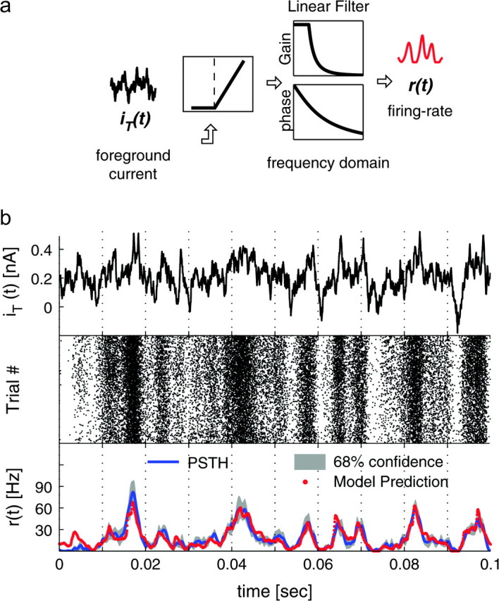
Prediction of the discharge response to a broadband input signal over a background noise. We challenged the significance of the linear response properties, searching for best-fit parameters of a phenomenological cascade model to predict the instantaneous firing rate in response to a broadband input i_T(t) (b—upper panel). Such a model, sketched in (a), has the structure of a classic Hammerstein model (Sakai 1992), where a static, or no-memory, threshold-linear element is followed by a linear system, as for the band-pass filters of Figures 5 and 6 (see the Methods). In (b), only the broadband current signal is shown (top), together with the corresponding spiking pattern elicited across different cycles and repetitions (middle). In the lower panel, the best-fit output r(t) of the model (red dots) was compared with the instantaneous firing probability (continuous blue line) obtained as a PSTH with a 68% confidence interval (gray shaded area), estimated over the corresponding raster plot (middle). The cascade model captures the input–output response properties of cortical neurons to fast inputs with acceptable accuracy (see Supplemental Table S3).

In summary, equations (5–7) describe a linear transformation preceded by a static, or no-memory, threshold-linear stage (eq. 4). The cascade ordering “nonlinear–linear” was preferred to “linear–nonlinear” for slightly better fit performances. All the parameters (i.e., P₁, P₂, G₀, {z_i},{π_i}, Δt) were adjusted to minimize the discrepancies between actual data and model predictions, employing Simulated Annealing techniques (Press et al. 1992). The chosen cost–function to minimize was represented by the χ² that quantified the mean quadratic discrepancy between actual data and model prediction, weighted by the confidence interval (Press et al. 1992). Large deviations are therefore weighted on the basis of the confidence on these data estimates. For the identification of the full cascade model in the time-domain, χ² was complemented by 1st-derivative mean discrepancies.

Statistics

Ninety-five percent confidence accuracy intervals on the nonlinear least-square parameter estimates were determined for r₀, r₁(f), and Φ(f) by the Levenberg–Marquardt fit algorithm, providing error bars in the plots of Figures 5 and 6 as in Fourcaud-Trocmé et al. (2003). For Figure 1b (lower panel) and Figure 6b, the gray shading represents the asymmetric 68% confidence accuracy interval (i.e., corresponding to 1 standard deviation) for the mean firing rate r_fix, as in Rauch et al. (2003).

In the case of identification of the phenomenological filter models, the χ²-test was used to evaluate the quality of the fits (Press et al. 1992), implicitly taking into account the number of free parameters.

Kendall's Tau nonparametric (rank-order) test (Press et al. 1992) was finally employed to assess correlations among spike-shape features and stimulation parameters, providing a measure c of correlation together with its significance level P, which represents the probability of obtaining the same value for c from statistically independent samples (i.e., false positive).

Results

The Linear Response to Time-Varying Noisy Inputs

Due to irregular spontaneous activity and the high degree of convergence, cortical neurons receive a continuous barrage of excitatory and inhibitory potentials in the intact brain. At the same time cortical cells participate in a variety of oscillations, whose frequency spans several orders of magnitude (e.g., 0.05–500 Hz) during distinct behavioral states (Buzsaki and Draguhn 2004). What is the impact of the background activity on neuronal responsiveness and on collective oscillations? We approached these issues by studying the linear response properties of single neurons characterizing their instantaneous discharge rate r(t) in response to a noisy background current with a small sinusoidal component, hereafter referred to as the “signal.” This allowed us not only to investigate how cortical neurons participate in an oscillatory regime, but especially how cells track temporally varying inputs under distinct background conditions (Fig. 1). We systematically varied the input oscillation frequency f, its amplitude I₁ and offset I₀, as well as the statistics (s, τ) of the background noise (eqs. 1 and 2). Because no correlation between the shape of the action potentials and these stimulation parameters was found, we restricted our analysis to the timing of each spike. However, very small correlations c exist between (I₀, I₁, s) and the maximal upstroke velocity and spike duration (|c| ≤ 0.1; P < 10⁻³), but they are consequence of nonideal bridge-balancing. Weak correlations c were instead found between the rat postnatal day and the spike upstroke velocity (c = 0.21; P < 10⁻¹²), downstroke velocity (c = −0.23; P < 10⁻¹⁴), and spike duration (c = −0.27; P < 10⁻¹⁹), as observed by many investigators.

The firing rate r(t) was estimated from the peristimulus time histograms (PSTHs) of the spike times over hundreds of cycles of the input current and over several stimulation trials. It was interpreted as the instantaneous discharge probability or, equivalently, as the firing rate of a cortical population composed of independent neurons.

In the limit of small-signal input amplitude I₁, r(t) could be well approximated by a sine wave oscillating at the same frequency f as the input current (Fig. 2c,d, upper panels):

(8)

r(t) is fully described in terms of mean firing rate r₀, modulation amplitude r₁(f), and phase-shift Φ(f) relative to the input current, as in linear dynamical transformations. At the beginning of each experiment, the stimulation parameters were selected in a way that r₀ was in the range 10–20 Hz, the membrane voltage fluctuations induced by the noise were 1–5 mV, and the discharge modulation amplitude r₁ was 0 < r₁ < r₀. Figure 2 reports typical spike responses evoked by input modulations at f = 10 Hz and at f = 250 Hz, recorded in the same cell. Individual firing times across successive input cycles and trial repetitions showed high variability (Fig. 2a,b, lower panels), as a consequence of the noise component uncorrelated with the sinusoidal signal oscillations.

Scaling the input amplitude I₁ in the range 20–200 pA while keeping I₀, s, and f fixed resulted in a linear scaling of the output amplitude r₁ (n = 3, not shown). However, for large input modulation depth (i.e. I₁ > 0.3 I₀), the amplitudes of output superimposed sinusoidal oscillations characterized by multiple frequencies of f (i.e., higher harmonic components) increased (n = 3), revealing the presence of input–output distortions as the limit of small input amplitude was exceeded. Thus, in most of the experiments we employed I₁ smaller than 30% of I₀, to fulfill the validity of the linear approximation where higher harmonics in the output could be neglected. Although similar values of I₁ are not infinitesimal with respect to I₀, this choice was confirmed to be reasonable by studying and predicting the neuronal discharge in response to more complex inputs signals across a wide range of firing rates, as discussed in the experiments of Figure 7.

Consistent with the hypothesis of linearity, no significant difference between the sum of the responses to individual sinusoids and the response to the sum of multiple sinusoids injected simultaneously was observed (Movshon et al. 1978; Victor 1979; Carandini et al. 1996) (n = 20, not shown).

Cortical Neurons Track Fast Inputs

Our experimental characterization aimed at identifying the linear neuronal response properties and at studying the way background noise affects them (Sakai 1992; Chichilnisky 2001; Fourcaud-Trocmé et al. 2003; Naundorf et al. 2005; Apfaltrer et al. 2006). In the framework of classic Fourier decomposition of any input signal to a neuron, r₁(f) and Φ(f) give quantitative information on how the neuronal encoding differentially attenuates and delays each frequency component f of the input, in the limit of small-signal amplitude.

Figure 3 summarizes population data and reports the unexpectedly wide bandwidth of the output temporal modulation depth r₁/r₀ and output phase-shift Φ. Although r₀ was unaffected by f, r₁ decreased significantly only for f > 100–200 Hz, regardless of the intensity and temporal correlations of the background noise. The profile of r₁(f) across frequencies did not match the membrane impedance, which was dominated by voltage-dependent resonances in the low-frequency range (i.e., 5–10 Hz—previously related to h-currents and M-currents) and by a low-pass behavior at high frequencies (not shown) with strong attenuation above 50 Hz (Gutfreund et al. 1995; Hutcheon et al. 1996).

Figure 3.

Modulation depth (r₁/r₀) and phase-shift Φ of the response to a noisy oscillatory input. The instantaneous firing rate r(t) evoked by small sinusoidal currents over a noisy background revealed sinusoidal oscillations with amplitude r₁ and phase-shift Φ, around a mean r₀ (quantified as in Fig. 2c,d). Surprisingly, pyramidal neurons can relay fast input modulations, up to several hundred cycles per second. The high-frequency response behavior matches a power-law relationship (i.e., r₁ ∼ f^α) with a linear phase-shift (i.e., Φ ∼ f). These plots were obtained for 67 cells, averaging across available repetitions and distinguishing between offset-currents I₀ above (suprathreshold regime) and below (subthreshold regime) the DC rheobase of the corresponding cell (as in Fig. 5). Data points corresponding to distinct input modulation frequencies were pooled together in nonoverlapping bins with size 0.1–10 Hz (low frequencies) and 100–200 Hz (high frequencies). Error bars represent the SE across the data points available (32 ± 25) for each bin. Markers shape and color identify the suprathreshold or weak-noise regime (black) and the subthreshold or strong-noise regime (red), characterized by distinct values for I₀ and s², adapted to yield a similar mean rate r₀ ∼ 20 Hz (i.e., 19.7 ± 1.5 Hz).

Above 200 Hz the output modulation depth decayed as a negative power-law, which appears as a straight (dashed) line in the double-logarithmic plot of Figure 3. The power-law exponent estimated by linear regression through the population data of Figure 3 was close to 2 (α = −1.80) and it matched the value obtained by averaging the exponents estimated in single experiments (α = −1.81 ± 0.31, n = 6—see Fig. 4a). A similar qualitative dependence, induced by system linearization, was anticipated by theoretical studies (Gerstner 2000; Knight 1972a) and could be replicated quantitatively in the case of integer power-law exponents through canonical phase oscillator models (Naundorf et al. 2005), nonlinear integrate-and-fire models (Fourcaud-Trocmé et al. 2003), and conductance-based neuronal modeling (Fourcaud-Trocmé et al. 2003). Integer values of α also relate to the number of best-fit free parameters of the phenomenological band-pass filters used in Figures 5–7 (see the Methods—eq. 6), introduced to fit the experimental data as discussed in the following sections.

Figure 4.

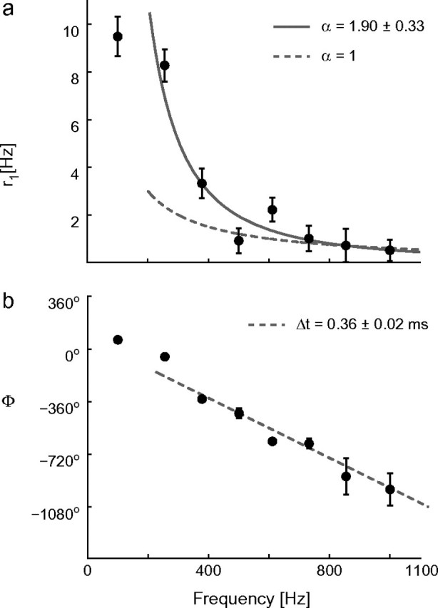
The high-frequency dynamical response properties of a typical cortical neuron, plotted in linear scale. The modulation amplitude (a) r₁(f), elicited by noisy oscillatory inputs, shows a power-law behavior (see also Fig. 3) captured by 1/f^α, with α ∼ 2, whereas the phase Φ of the response (b) decreases linearly with increasing frequencies f (i.e., Φ → −360°·f·Δt). Stimulation parameters (I₀, I₁, s) = (400, 150, 500) pA and τ = 5 ms.

Even though the inspection of Figure 3 seems to indicate that the points at highest frequencies can be fitted by 1/f, Figure 4a supports the conclusion that 1/f² is a more precise characterization. Nevertheless, numerical simulations showed that the high-frequency asymptotic behavior might be reached at frequencies which are much higher than the cut-off frequency (Fourcaud-Trocmé et al. 2003), so that assessing the precise value of α might not be conclusive on the basis of our observations.

As opposed to typical linear systems, the phase-shift at high frequencies did not saturate but decreased linearly with f (see Fig. 4b). This is reminiscent of the presence of a constant time delay Δt between input and output. This delay was in the range 0.3–1.1 ms, sometimes much larger than the “threshold-to-peak voltage” lag ${\text{τ}}_{\text{sp}}$ during a spike. ${\text{τ}}_{\text{sp}}$ quantifies the rising phase of each action potential, upon conventional definition of “threshold” as the membrane voltage corresponding to a rate of change of 10 mV/ms, and it was in the range of 0.3–0.5 ms. As expected from the previous report (Fourcaud-Trocmé et al. 2003), Δt^model was always equal to ${\text{τ}}_{\text{sp}}$ in single-compartmental computer simulations (not shown). However, the mismatch between ${\text{τ}}_{\text{sp}}$ and Δt observed in some cells might be explained in terms of relevant additional axo-somatic and somato-axonic propagation latencies of about 0.2 ms each. This was measured directly by Palmer and Stuart (2006), who reported that cortical cells initiate action potentials at the distal end of the initial axon segment (see also Shu et al. 2006).

The Background Noise Affects the Neuronal Dynamical Response at Intermediate Frequencies

In the absence of background fluctuations, a neuron discharges only when its input current surpasses a certain threshold (i.e., the rheobase current). When the input current is noisy and fluctuations are induced in the membrane voltage, the neuron can be brought to spiking even when its average input is below the threshold (i.e., “subthreshold”). Thus, the mean firing rate of the neuron r₀ is determined by both the mean current I₀ and the standard deviation s of the noise. At the beginning of each experiment, I₀ and s were tuned to obtain the same mean firing rate r₀, chosen in the range 10–20 Hz. This allowed us to evoke 2 different discharge regimes, reflected in the degree of the irregular firing: the suprathreshold or weak-noise regime and the subthreshold or strong-noise regime. In the weak-noise regime, the background input fluctuation amplitude s was set to 20–50 pA and its mean I₀ was chosen above rheobase. Conversely, in the strong-noise regime, I₀ was set below rheobase, and s was increased until r₀ matched the value obtained in the suprathreshold regime.

Figure 5 summarizes the results of these experiments, reporting the responses of 4 typical cells (see also Fig. 3). It shows that the intensity s of the background noise, mimicking presynaptic firing as well as presynaptic background cross-correlations (Rudolph and Destexhe 2004), differentially affects the neuronal response. This occurs especially at intermediate frequencies, flattening the response profile, and smoothening resonances as predicted in theoretical studies (Knight 1972a; Brunel et al. 2001; Fourcaud-Trocmé et al. 2003; Richardson et al. 2003). The modulation of the neuronal discharge does not appear significantly attenuated at frequencies lower than 100–300 Hz in both regimes (see also Fig. 2), as for Figure 3 but plotted in linear instead of logarithmic scale for the vertical axis. At low input frequencies f (1–20 Hz), an increase in r₁ and a phase-advance were always observed (see Figs 5 and 6). These effects are apparent when analyzing single-cell responses rather than population averages (compare Figs 3 and 5).

In general, uniform and dense sampling of the frequency axis was not practicable, given the limited time window for stability and reproducibility of the neuronal response in typical recordings (see the Methods). This resulted in privileging high frequencies in some experiments (e.g., see Fig. 4) while neglecting intermediate frequencies in others, and vice versa (e.g., Fig. 6). This prompted us to test a posteriori whether data points collected simultaneously on the response magnitude r₁ and phase Φ were consistent with the hypothesis of linearity, while providing meaningful interpolations between samples (see Fig. 5d). In fact, the mutual relationship between r₁ and phase Φ cannot be arbitrary in a linear system. Therefore, a filter model (eqs. 6 and 7, see the Methods) was routinely employed to fit the data from each experiment. This model captured the neuronal response to the input signal component and its best-fit attenuation and phase-shift were plotted in Figures 5 and 6 as thick continuous lines. As in electrical filters made of linear resistors, capacitors and inductors (Horowitz and Hill 1989), the number and location of the model intrinsic time-constants account for integer power-law behavior and for low frequencies resonances and phase-advance, while matching the profiles of r₁ and Φ simultaneously. Changing the background noise level (black and red colors in Figs 3 and 5) resulted only in a shift in the best-fit values of the intrinsic time-constants of the model and required no modification of their number. This shift was smaller for faster time-constants (i.e., less than ± 30%, for time constants below ∼3 ms—see Supplemental Table S1), indicating that the high-frequency response of the neuron was generally unaffected by the noise intensity.

Background Temporal Correlations Do Not Speed up Neuronal Reaction Times

The timescale of background fluctuations (i.e., the “color” of the noise) was systematically varied in our experiments (Fig. 6). This is set by the correlation time τ of the noise (eq. 2) that mimics the decay time-constant of synaptic currents. In previous theoretical studies, the dependence of Φ on τ was emphasized (Brunel et al. 2001), suggesting that synaptic noise might have an impact on the reaction times to fast inputs transients reducing the response phase-lag to zero and removing amplitude attenuations (Knight 1972a; Gerstner 2000). Here, we explored the effect of changing the values of τ in the range 5–100 ms, thereby mimicking the contribution of fast (AMPA- and GABA_A-mediated), slow (NMDA- and GABA_B-mediated) synaptic currents. Both Φ and r₁ showed sensitivity to τ for intermediate frequencies, but not in the high-frequency regime, as plotted in Figure 6 for 4 typical cells. This is consistent with the results of the simulations of a conductance-based model neuron (not shown), and with the predictions of Fourcaud-Trocmé et al. (2003).

As discussed in the previous section and shown in Figure 5, r₁(f) and $\text{Φ}(f)$ could be simultaneously fit by the frequency response of a linear filter model. A change of the noise time-constant τ shifted the best-fit parameters, but required no modification of their number. The shift was smaller for faster time-constants (i.e., less than ± 20%, for time constants generally below ∼3 ms—see Supplemental Table S2).

Significance of the Linear Response Properties to Predict Neuronal Responses

The good accuracy of the linear filter to fit the experimental data (Figs 5 and 6, continuous lines) prompted us to test up to which extend linear properties dominate the input–output response in pyramidal neurons. In fact, ideal linear systems process each Fourier-component of their input independently and distortion-free, so that the frequency-domain response of the system is sufficient to predict the corresponding output.

We investigated the response r(t) to a broadband signal i_T(t), instead of sinusoids (see the Methods). With the aim of approaching the conditions of the periodic regime studied in the previous sections, i_T(t) was cyclically repeated with a period of T = 100 ms. With the additional background noise, these experiments generalize and extend those of Mainen and Sejnowski (1995), who looked at fast stimulus transients and neuronal response reliability. Furthermore, our approach allows one to study the response of a cortical population, where neurons experience uncorrelated background activity, weakly interacting with each other and receiving the same input signal. In Figure 7b, a sample waveform of the broadband input was plotted, together with the raster-plots of the spikes evoked across hundreds of cycles and repetitions. In analogy to the analysis shown in Figure 2, the peristimulus time histograms (PSTHs) computed from the raster-plot was used to estimate the instantaneous firing rate r(t).

Although instantaneous input amplitudes were not small compared with I₀, the phenomenological filter employed in Figures 5 and 6 could predict the time-varying neuronal response with satisfying accuracy over a wide range of output firing rates (Fig. 7), tracking fast input transients. However, to account for large negative input amplitudes that occasionally occur, a minimal current-threshold was needed in cascade to the linear filter (eqs. 4, 6, and 7). Without it, the correct dynamical range of the response could not be replicated and the fitting procedure led to low prediction performances. The order “nonlinear–linear”, sketched in Figure 7a, was preferred to the “linear–nonlinear” (Sakai 1992) as it systematically led to slightly superior fit performances, as well as to a possible interpretation as the neuronal rheobase.

Discussion

In the present work we studied the basic questions of how neurons encode time-varying inputs into spike trains, how efficiently they achieve it and what the impact of the background noise is. This is of central importance to understand network activities like network-driven persistent oscillatory regimes, which depend on the single-cell dynamical response properties and on recurrent connectivity.

Previous studies used deterministic oscillating inputs in invertebrate (Knight 1972b; French et al. 2001) and vertebrate neurons in hippocampus and entorhinal cortex (Schreiber et al. 2004), in thalamocortical neurons (Smith et al. 2000), in spinal interneurons and motoneurons (Baldissera et al. 1984), in the vestibular system (du Lac and Lisberger 1995; Ris et al. 2001), in the auditory (Liu et al. 2006), and visual systems (Victor and Shapley 1979a, 1979b; Sakai 1992; Carandini et al. 1996; Nowak et al. 1997), with emphasis on spike timing and reliability (Fellous et al. 2001; Schaette et al. 2005) and synchronization (Gutkin et al. 2005). Our results extend those studies in 2 ways: 1) by examining the contribution of background fluctuations and 2) by systematically exploring the dynamical response properties up to the high-frequency range (1 kHz).

By the interpretation of the instantaneous firing rate as a population activity, our analysis suggests that cortical ensembles are extremely efficient in tracking transients that are much faster than the membrane time-constant (∼20 ms—see the Methods) and the average interspike interval (∼1/r₀ ≅ 50 ms) of individual cells. This finding was anticipated by many theoretical studies and it correlates with the previous observations that single cortical neurons (Mainen and Sejnowski 1995) and hypoglossal motoneurons (Powers et al. 2005) may have phase-locked firing responses to fast-varying current inputs, as well as with the study of Bair and Koch (1996), who observed large cut-off frequencies in the power spectra of the responses of middle temporal cortical neurons to in vivo random visual stimulation. However, our results extend the previous studies to the case of high-frequency phase-locking of the population firing rates, under noisy background. Although this is not unexpected (Knight 1972a), our findings disprove that the noise and its temporal correlations make a neuronal population respond instantaneously to an input (Knight 1972a; Gerstner 2000; Brunel et al. 2001; Silberberg et al. 2004). In fact, both noise intensity s and correlation time τ modulate the neuronal response only at low and intermediate input frequencies and do not affect the low-pass filtering profile of the response, in agreement with Fourcaud-Trocmé et al. (2003) and with Naundorf et al. (2005).

The location of the observed cut-off frequency was higher than the predictions from single-compartmental conductance based model neurons (Fourcaud-Trocmé et al. 2003). In those studies, the cut-off was of the order of r₀ and increased with the increasing sharpness of the action potentials. Similarly, Naundorf et al. (2005) observed an increase in the neuronal response at input frequencies much higher than r₀ (i.e. up to 200 Hz) for increasing action potential onset speed, while studying a phase-oscillator point neuron model. We propose that the effective spike sharpness could be higher than what was previously modeled at the soma. We speculate that a multicompartmental description that incorporates the details of axonic spike initiation (McCormick et al. 2007; Shu et al. 2007) might quantitatively support our experimental observations.

We observed a phase-advance at low input frequencies that was previously interpreted mechanistically on the basis of ion currents responsible for spike-frequency adaptation (Fleidervish et al. 1996; Ahmed et al. 1998; Fuhrmann et al. 2002; Compte et al. 2003; Paninski et al. 2003), as well as of resonances of the membrane impedance (Brunel et al. 2003; Richardson et al. 2003). These hypotheses are consistent with the input frequency range ∼1–10 Hz (i.e. (100 ms)⁻¹–(1000 ms)⁻¹) of the phase-advance and with its sensitivity to the levels of the background noise we observed in our experiments.

The use of current-clamp was a meaningful choice for an immediate comparison to the analytical and numerical studies of Fourcaud-Trocmé et al. (2003), Geisler et al. (2005) and many others. A more realistic somatic conductance–injection is expected to change quantitatively but not qualitatively our conclusions (see also Apfaltrer et al. 2006). Even when excitatory and inhibitory fluctuating conductances significantly alter the effective membrane time-constant τ_m of the neuron (Destexhe et al. 2003), their additional temporal modulation will not affect further τ_m, in the limit of small amplitude considered here. Previous theoretical studies directly showed that the location of the cut-off frequency as well as of the resonances due to subthreshold resonances (Richardson et al. 2003) shift with distinct conductance-states of the neuron, but pointed out that the power-law exponent α and the sensitivity to the background noise remain unaffected (Fourcaud-Trocmé et al. 2003; Geisler et al. 2005). Nevertheless, in order to carefully extend the discussion of Rauch et al. (2003) (see also La Camera et al. 2004; Richardson and Gerstner 2005) towards a mapping between the dynamical response properties induced by current-driven stimuli to those induced by conductance-driven stimuli, our results will require to be reevaluated under dynamic-clamp recordings (Robinson 1994; Destexhe et al. 2001).

The response amplitude r₁(f) decays as a power-law in the high-frequency range and the exponent α of the power-law 1/f^α was approximately 2. This is in contrast to what is predicted for the Wang-Buzsaki model (Wang and Buzsaki 1996) and for the exponential integrate-and-fire neuron (Fourcaud-Trocmé et al. 2003), but it is consistent with a polynomial V–I dependence of the spike-initiating mechanisms (not shown). This steeper power-law is unlikely a measurement artifact. The glass pipette used to inject sinusoidal input currents has indeed low-pass filter properties in “cascade” to the neuron. However, these filtering properties occur mainly between input–output voltages due to parallel parasitic capacitances. Input–output currents are unlikely to be prefiltered due to inductive electrical effects and viscosity in the movement of charge carriers in the pipette solutions, as these are negligible phenomena in the frequency range we investigated.

Finally, the local slope (i.e., gain) of the static f–I curve affects neuronal responses regardless of the input modulation frequencies (Fourcaud-Trocmé et al. 2003). Previously reported gain-modulations induced by background noise (Chance et al. 2002; Higgs et al. 2006) are qualitatively distinct than the effects shown in Figures 5 and 6, as they act by scaling the firing rate output of the neurons across all the input frequency-bands.

Our experimental results then suggest that the action potential is a major evolutionary breakthrough, not only for making possible long-distance propagation of signals, but more importantly because it represents a powerful large-bandwidth digital intercellular communication channel, through population coding. In fact, our work shows that population coding with spikes has no significant attenuation in the range 0–200 Hz, while it compensates the heavy drawbacks of the analog intracellular membrane properties, which filter out input frequencies faster than ∼50 Hz.

Relations to Reverse-Correlation Methods

Neural coding and the dynamical characterization of the input–output transformation operated by neurons, have been previously addressed by using methods of stimulus reconstruction (Bialek et al. 1991; Rieke et al. 1995) or reverse correlation (de Boer and Kuyper 1968; Gerstner and Kistler 2002). The last identifies the typical input current preceding a spike. Such a procedure estimates the 1st-order Wiener kernel and thus the linear component of the system (Kroller 1992) even though underlying nonlinearities might be present “in cascade” (Chichilnisky 2001). The reverse correlation kernel is proportional to the impulse response of the linear response of the neuron and it characterizes the “meaning” of each spike (Kroller 1992). The frequency-domain characterization that we considered so far directly relates to such an impulse response upon Fourier transform, although here we focused only on the encoding of the input signal (and not of the overall waveform) into the output. We thus generalized the previous experimental investigations to include the effect of background noise.

Consistently with the weak impact of background noise at high input frequencies that we reported, one might expect that similar cut-off frequencies (i.e. ∼100–200 Hz) were quantitatively observed by previous investigators, although they might have not included any background noise. For instance, the “stimulus kernel” identified by Powers et al. (2005) in motoneurons by injecting stationary “white”-noise inputs, appears to be dominated by a single decay time-constant in the order of 5–10 ms, indeed matching the 100–200 Hz cut-off frequencies of our data. Similarly, the low-noise phase-advance properties we observed (e.g., Fig. 2a) and the filter model intrinsic (high-pass) time-constants identified in our experiments, quantitatively correlate with the “feed-back” kernel computed by the same authors after selecting short and long interspike-intervals to unveil the effect of spike-frequency adaptation.

Finally, with the aim of further exploring the relationship of our approach with the previous ones, we directly computed the spike-triggered average (STA) of the input current preceding a spike, in 3 experiments where a broadband signal i_T(t) was injected. In Figure 8, we compare the Fourier transform of the STA to the frequency response of the best-fit linear filter model optimized to match the instantaneous firing rate (as in Fig. 7). As expected interpreting the STA as the 1st-order kernel reveals striking similarities between the 2 approaches, especially for frequencies higher than 200 Hz.

Figure 8.

Comparison between the 1st-order kernels computed by reverse-correlation techniques and the best-fit frequency response of the linear filter model of Figure 7. The modulation amplitude r₁(f) (dashed line, identifying eq. 6) was compared with the fast Fourier transform (FFT) of the STA (markers) of the input current preceding a spike. The last was evaluated correlating the signal component i_T(t) with the timing of each action potential, in 3 experiments. As expected from interpreting the STA as the 1st-order kernel, striking similarities are apparent.

The Phenomenological Filter Model

Linear response properties are relevant to predict the response to complex noisy waveforms, even though the hypothesis of small input amplitude was not strictly respected by i_T(t). As discussed by Carandini et al. (1996), our experiments support the idea that in vivo membrane potential fluctuations linearize the response to stimulus-related input components (Masuda et al. 2005). Consistently, the neuronal response r(t) could not be captured by employing a static nonlinearity alone (not shown), even though for stationary noisy stimuli a similar description is appropriate (Rauch et al. 2003; Giugliano et al. 2004; La Camera et al. 2006; Arsiero et al. 2007). The additional cascade threshold-linear element simply relates to the presence of a minimal input threshold. It is interesting to note that the piecewise-linear profile of such nonlinearity reflects the minor role played by distortions and harmonics in our experiments.

Summarizing, a simple “cascade” model could quantitatively capture the time course of the instantaneous discharge rate (see also Shelley et al. 2002; Gutkin et al. 2005; Schaette et al. 2005), although it neglected the precise firing times. On the other hand, these can be captured by spiking neuron models, as in Jolivet et al. (2006) and Paninski (2006), identifying the parameters of an exponential (or quadratic) integrate-and-fire including spike-frequency adaptation as in Brette and Gerstner (2005).

Cortical Rhythms

Slow inputs produced a phase-advance of the output response whereas fast inputs a phase-lag, relative to the input modulation (Fuhrmann et al. 2002). This has been proposed to have important consequences for emerging population dynamics in recurrent networks, as the signals propagation between pre- and postsynaptic spikes does not only depend on the synaptic delays but also on the (oscillation frequency-dependent) delay introduced by the postsynaptic neuron itself. The fact that spike timing depends on f is particularly relevant for the emergence of population rhythms including fast ripples (Buzsaki et al. 1992; Csicsvari et al. 1999; Grenier et al. 2003; Buzsaki and Draguhn 2004; Buzsaki et al. 2004). In fact, the spikes of a presynaptic neuron, which is engaged in network-driven oscillations, generate periodic synaptic currents. Then the postsynaptic neuron experiences the periodic maxima of these currents after a synaptic delay, and responds to such a current signal reaching the maximum of its firing rate with an additional delay Φ(f) and attenuation r₁/I₁. If both presynaptic and postsynaptic neurons are participating in the same global rhythm, the overall delay between the pre- and postsynaptic spikes must be consistent with the period of the global oscillation and no strong attenuation should occur at that frequency, as shown in computer simulations by Fuhrmann et al. (2002), Brunel and Wang (2003), and Geisler et al. (2005). Therefore, not every oscillation frequency f is compatible with a given recurrent network architecture, synaptic coupling and firing regime.

We showed that the phase-shift and response amplitude of L5 pyramidal cells depends on the background fluctuations (Figs 5 and 6). This suggests that the frequency of emerging rhythms can be modulated by a background network embedding those neurons, as the phase of single-cell response is affected. More general, any network activity that relies on the timing of recurrent spikes is governed not only by the synaptic dynamics but is also controlled by the response properties (Φ(f), r₁) of single cells.

Funding

Swiss National Science Foundation grant (No. 31-61335.00) to H.-R.L.; the Silva Casa foundation, the National Institute of Mental Health grant (2R01MH-62349), and the Swartz Foundation to C.G. and X.-J.W.; and the Human Frontier Science Program (LT00561/2001-B) to M.G.

Supplementary Material

Supplementary material can be found at: http://www.cercor.oxfordjournals.org/

References

- Ahmed B, Anderson JC, Douglas RJ, Martin KA, Whitteridge D. Estimates of the net excitatory currents evoked by visual stimulation of identified neurons in cat visual cortex. Cereb Cortex. 1998;8(5):462–476. doi: 10.1093/cercor/8.5.462. [DOI] [PubMed] [Google Scholar]
- Apfaltrer F, Ly C, Tranchina D. Population density methods for stochastic neurons with realistic synaptic kinetics: firing rate dynamics and fast computational methods. Netw Comput Neural Sys. 2006;17(4):373–418. doi: 10.1080/09548980601069787. [DOI] [PubMed] [Google Scholar]
- Arsiero M, Lüscher H-R, Lundstrom BN, Giugliano M. The impact of input fluctuations on the frequency-current relationships of layer 5 pyramidal neurons in the rat medial prefrontal cortex. J Neurosci. 2007;27(12):3274–3284. doi: 10.1523/JNEUROSCI.4937-06.2007. [DOI] [PMC free article] [PubMed] [Google Scholar]
- Bair W, Koch C. Temporal precision of spike trains in extrastriate cortex of the behaving macaque monkey. Neural Comput. 1996;8:1185–1202. doi: 10.1162/neco.1996.8.6.1185. [DOI] [PubMed] [Google Scholar]
- Baldissera F, Campadelli P, Piccinelli L. The dynamic response of cat alpha-motoneurones investigated by intracellular injection of sinusoidal currents. Exp Brain Res. 1984;54(2):275–282. doi: 10.1007/BF00236227. [DOI] [PubMed] [Google Scholar]
- Bialek W, Rieke F, de Ruyter van Steveninck RR, Warland D. Reading a neural code. Science. 1991;252(5014):1854–1857. doi: 10.1126/science.2063199. [DOI] [PubMed] [Google Scholar]
- Brette R, Gerstner W. Adaptive exponential integrate-and-fire model as an effective description of neuronal activity. J Neurophysiol. 2005;94(5):3637–3642. doi: 10.1152/jn.00686.2005. [DOI] [PubMed] [Google Scholar]
- Brogan WL. Modern control theory. Englewood Cliffs (NJ): Prentice Hall; 1991. [Google Scholar]
- Brunel N, Chance FS, Fourcaud N, Abbott LF. Effects of synaptic noise and filtering on the frequency response of spiking neurons. Phys Rev Lett. 2001;86(10):2186–2189. doi: 10.1103/PhysRevLett.86.2186. [DOI] [PubMed] [Google Scholar]
- Brunel N, Hakim V, Richardson MJE. Firing-rate resonance in a generalized integrate-and-fire neuron with subthreshold resonance. Phys Rev E Stat Nonlin Soft Matter Phys. 2003;67(5 Pt 1):051916. doi: 10.1103/PhysRevE.67.051916. [DOI] [PubMed] [Google Scholar]
- Brunel N, Wang X-J. What determines the frequency of fast network oscillations with irregular neural discharges? I. Synaptic dynamics and excitation-inhibition balance. J Neurophysiol. 2003;90(1):415–430. doi: 10.1152/jn.01095.2002. [DOI] [PubMed] [Google Scholar]
- Buzsaki G, Draguhn A. Neuronal oscillations in cortical networks. Science. 2004;304(5679):1926–1929. doi: 10.1126/science.1099745. [DOI] [PubMed] [Google Scholar]
- Buzsaki G, Geisler C, Hinze D, Wang X-J. Circuit complexity and axon wiring economy of cortical interneurons. Trends Neurosci. 2004;27(4):186–193. doi: 10.1016/j.tins.2004.02.007. [DOI] [PubMed] [Google Scholar]
- Buzsaki G, Horvath Z, Urioste R, Hetke J, Wise K. High-frequency network oscillation in the hippocampus. Science. 1992;256(5059):1025–1027. doi: 10.1126/science.1589772. [DOI] [PubMed] [Google Scholar]
- Carandini M, Mechler F, Leonard CS, Movshon JA. Spike train encoding by regular-spiking cells of the visual cortex. J Neurophysiol. 1996;76(5):3425–3441. doi: 10.1152/jn.1996.76.5.3425. [DOI] [PubMed] [Google Scholar]
- Chance FS, Abbott LF, Reyes AD. Gain modulation from background synaptic input. Neuron. 2002;35(4):773–782. doi: 10.1016/s0896-6273(02)00820-6. [DOI] [PubMed] [Google Scholar]
- Chichilnisky EJ. A simple white noise analysis of neuronal light responses. Network. 2001;12(2):199–213. [PubMed] [Google Scholar]
- Compte A, Sanchez-Vives MV, McCormick DA, Wang X-J. Cellular and network mechanisms of slow oscillatory activity (<1 Hz) and wave propagations in a cortical network model. J Neurophysiol. 2003;89(5):2707–2725. doi: 10.1152/jn.00845.2002. [DOI] [PubMed] [Google Scholar]
- Csicsvari J, Hirase H, Czurko A, Mamiya A, Buzsaki G. Oscillatory coupling of hippocampal pyramidal cells and interneurons in the behaving rat. J Neurosci. 1999;19(1):274–287. doi: 10.1523/JNEUROSCI.19-01-00274.1999. [DOI] [PMC free article] [PubMed] [Google Scholar]
- de Boer R, Kuyper P. Triggered correlation. IEEE Trans Biomed Eng. 1968;15(3):169–179. doi: 10.1109/tbme.1968.4502561. [DOI] [PubMed] [Google Scholar]
- Destexhe A, Rudolph M, Fellous JM, Sejnowski TJ. Fluctuating synaptic conductances recreate in vivo-like activity in neocortical neurons. Neuroscience. 2001;107(1):13–24. doi: 10.1016/s0306-4522(01)00344-x. [DOI] [PMC free article] [PubMed] [Google Scholar]
- Destexhe A, Rudolph M, Paré D. The high-conductance state of neocortical neurons in vivo. Nat Rev Neurosci. 2003;4(9):739–751. doi: 10.1038/nrn1198. [DOI] [PubMed] [Google Scholar]
- du Lac S, Lisberger SG. Cellular processing of temporal information in medial vestibular nucleus neurons. J Neurosci. 1995;15(12):8000–8010. doi: 10.1523/JNEUROSCI.15-12-08000.1995. [DOI] [PMC free article] [PubMed] [Google Scholar]
- Fellous JM, Houweling AR, Modi RH, Rao RP, Tiesinga PH, Sejnowski TJ. Frequency dependence of spike timing reliability in cortical pyramidal cells and interneurons. J Neurophysiol. 2001;85(4):1782–1787. doi: 10.1152/jn.2001.85.4.1782. [DOI] [PubMed] [Google Scholar]
- Fleidervish IA, Friedman A, Gutnick MJ. Slow inactivation of Na+ current and slow cumulative spike adaptation in mouse and guinea-pig neocortical neurons in slices. J Physiol. 1996;493(Pt 1):83–97. doi: 10.1113/jphysiol.1996.sp021366. [DOI] [PMC free article] [PubMed] [Google Scholar]
- Fourcaud-Trocmé N, Brunel N. Dynamics of the instantaneous firing rate in response to changes in input statistics. J Comput Neurosci. 2005;18(3):311–321. doi: 10.1007/s10827-005-0337-8. [DOI] [PubMed] [Google Scholar]
- Fourcaud-Trocmé N, Hansel D, van Vreeswijk C, Brunel N. How spike generation mechanisms determine the neuronal response to fluctuating inputs. J Neurosci. 2003;23(37):11628–11640. doi: 10.1523/JNEUROSCI.23-37-11628.2003. [DOI] [PMC free article] [PubMed] [Google Scholar]
- French AS. Practical nonlinear system analysis by wiener kernel estimation in the frequency domain. Biol Cybern. 1976;24:111–119. [Google Scholar]
- French AS, Hoger U, Sekizawa S, Torkkeli PH. Frequency response functions and information capacities of paired spider mechanoreceptor neurons. Biol Cybern. 2001;85(4):293–300. doi: 10.1007/s004220100260. [DOI] [PubMed] [Google Scholar]
- Fuhrmann G, Markram H, Tsodyks M. Spike frequency adaptation and neocortical rhythms. J Neurophysiol. 2002;88(2):761–770. doi: 10.1152/jn.2002.88.2.761. [DOI] [PubMed] [Google Scholar]
- Geisler C, Brunel N, Wang X-J. Contributions of intrinsic membrane dynamics to fast network oscillations with irregular neuronal discharges. J Neurophysiol. 2005;94(6):4344–4361. doi: 10.1152/jn.00510.2004. [DOI] [PubMed] [Google Scholar]
- Gerstner W. Population dynamics of spiking neurons: fast transients, asynchronous states, and locking. Neural Comput. 2000;12(1):43–89. doi: 10.1162/089976600300015899. [DOI] [PubMed] [Google Scholar]
- Gerstner W, Kistler W. Spiking neuron models: single neurons, populations, plasticity. Cambridge (UK): Cambridge University Press; 2002. [Google Scholar]
- Giugliano M, Darbon P, Arsiero M, Lüscher H-R, Streit J. Single-neuron discharge properties and network activity in dissociated cultures of neocortex. J Neurophysiol. 2004;92(2):977–996. doi: 10.1152/jn.00067.2004. [DOI] [PubMed] [Google Scholar]
- Grenier F, Timofeev I, Steriade M. Neocortical very fast oscillations (ripples, 80-200 Hz) during seizures: intracellular correlates. J Neurophysiol. 2003;89(2):841–852. doi: 10.1152/jn.00420.2002. [DOI] [PubMed] [Google Scholar]
- Gutfreund Y, Yarom Y, Segev I. Subthreshold oscillations and resonant frequency in guinea-pig cortical neurons: physiology and modeling. J Physiol. 1995;483:621–640. doi: 10.1113/jphysiol.1995.sp020611. [DOI] [PMC free article] [PubMed] [Google Scholar]
- Gutkin BS, Ermentrout GB, Reyes AD. Phase-response curves give the responses of neurons to transient inputs. J Neurophysiol. 2005;94(2):1623–1635. doi: 10.1152/jn.00359.2004. [DOI] [PubMed] [Google Scholar]
- Higgs MH, Slee SJ, Spain WJ. Diversity of gain modulation by noise in neocortical neurons: regulation by the slow afterhyperpolarization conductance. J Neurosci. 2006;26(34):8787–8799. doi: 10.1523/JNEUROSCI.1792-06.2006. [DOI] [PMC free article] [PubMed] [Google Scholar]
- Horowitz P, Hill W. The art of electronics. 2nd ed. Cambridge (UK): Cambridge University Press; 1989. [Google Scholar]
- Hsu SM, Raine L, Fanger H. Use of avidin-biotin-peroxidase complex (ABC) in immunoperoxidase techniques: a comparison between ABC and unlabeled antibody (PAP) procedures. J Histochem Cytochem. 1981;29(4):577–580. doi: 10.1177/29.4.6166661. [DOI] [PubMed] [Google Scholar]
- Hutcheon B, Miura RM, Puil E. Subthreshold membrane resonance in neocortical neurons. J Neurophysiol. 1996;76(2):683–697. doi: 10.1152/jn.1996.76.2.683. [DOI] [PubMed] [Google Scholar]
- Iansek R, Redman SJ. An analysis of the cable properties of spinal motoneurones using a brief intracellular current pulse. J Physiol. 1973;234:613–636. doi: 10.1113/jphysiol.1973.sp010364. [DOI] [PMC free article] [PubMed] [Google Scholar]
- Jolivet R, Rauch A, Lüscher HR, Gerstner W. Predicting spike timing of neocortical pyramidal neurons by simple threshold models. J Comput Neurosci. 2006;21(1):35–49. doi: 10.1007/s10827-006-7074-5. [DOI] [PubMed] [Google Scholar]
- Kim KJ, Rieke F. Temporal Contrast Adaptation in the Input and Output Signals of Salamander Retinal Ganglion Cells. J Neurosci. 2001;21(1):287–299. doi: 10.1523/JNEUROSCI.21-01-00287.2001. [DOI] [PMC free article] [PubMed] [Google Scholar]
- Knight BW. Dynamics of encoding in a population of neurons. J Gen Physiol. 1972a;59(6):734–766. doi: 10.1085/jgp.59.6.734. [DOI] [PMC free article] [PubMed] [Google Scholar]
- Knight BW. The relationship between the firing rate of a single neuron and the level of activity in a population of neurons. Dynamics of encoding in a population of neurons. J Gen Physiol. 1972b;59(6):767–778. doi: 10.1085/jgp.59.6.767. [DOI] [PMC free article] [PubMed] [Google Scholar]
- Kroller J. Band-limited white noise stimulation and reverse correlation analysis in the prediction of impulse responses of encoder models. Biol Cybern. 1992;67:207–215. [Google Scholar]
- La Camera G, Rauch A, Thurbon D, Lüscher HR, Senn W, Fusi S. Multiple time scales of temporal response in pyramidal and fast spiking cortical neurons. J Neurophysiol. 2006;96(6):3448–3464. doi: 10.1152/jn.00453.2006. [DOI] [PubMed] [Google Scholar]
- La Camera G, Senn W, Fusi S. Comparison between networks of conductance- and current-driven neurons: stationary spike rates and subthreshold depolarization. Neurocomputing. 2004;58-60:253–258. [Google Scholar]
- Liu LF, Palmer AR, Wallace MN. Phase-locked responses to pure tones in the inferior colliculus. J Neurophysiol. 2006;95(3):1926–1935. doi: 10.1152/jn.00497.2005. [DOI] [PubMed] [Google Scholar]
- Mainen ZF, Sejnowski TJ. Reliability of spike timing in neocortical neurons. Science. 1995;268(5216):1503–1506. doi: 10.1126/science.7770778. [DOI] [PubMed] [Google Scholar]
- Masuda N, Doiron B, Longtin A, Aihara K. Coding of temporally varying signals in networks of spiking neurons with global delayed feedback. Neural Comp. 2005;17(10):2139–2175. doi: 10.1162/0899766054615680. [DOI] [PubMed] [Google Scholar]
- McCormick DA, Connors BW, Lighthall JW, Prince DA. Comparative electrophysiology of pyramidal and sparsely spiny stellate neurons of the neocortex. J Neurophysiol. 1985;54(4):782–806. doi: 10.1152/jn.1985.54.4.782. [DOI] [PubMed] [Google Scholar]
- McCormick DA, Shu Y, Yu Y. Neurophysiology: Hodgkin and Huxley model—still standing? Nature. 2007;445(7123):E1–E2. doi: 10.1038/nature05523. [DOI] [PubMed] [Google Scholar]
- Movshon JA, Thompson ID, Tolhurst DJ. Spatial summation in the receptive fields of simple cells in the cat's striate cortex. J Physiol. 1978;283:53–77. doi: 10.1113/jphysiol.1978.sp012488. [DOI] [PMC free article] [PubMed] [Google Scholar]
- Naundorf B, Geisel T, Wolf F. Action potential onset dynamics and the response speed of neuronal populations. J Comput Neurosci. 2005;18:297–309. doi: 10.1007/s10827-005-0329-8. [DOI] [PubMed] [Google Scholar]
- Nowak L, Sanchez-Vives M, McCormick D. Influence of low and high frequency inputs on spike timing in visual cortical neurons. Cereb Cortex. 1997;7:487–501. doi: 10.1093/cercor/7.6.487. [DOI] [PubMed] [Google Scholar]
- Palmer LM, Stuart GJ. Site of action potential initiation in layer 5 pyramidal neurons. J Neurosci. 2006;26(6):1854–1863. doi: 10.1523/JNEUROSCI.4812-05.2006. [DOI] [PMC free article] [PubMed] [Google Scholar]
- Paninski L. The spike-triggered average of the integrate-and-fire cell driven by gaussian white noise. Neural Comput. 2006;18(11):2592–2616. doi: 10.1162/neco.2006.18.11.2592. [DOI] [PubMed] [Google Scholar]
- Paninski L, Lau B, Reyes A. Noise-driven adaptation: in vitro and mathematical analysis. Neurocomputing. 2003;52:877–883. [Google Scholar]
- Paré D, Shink E, Gaudreau H, Destexhe A, Lang EJ. Impact of spontaneous synaptic activity on the resting properties of cat neocortical pyramidal neurons in vivo. J Neurophysiol. 1998;79(3):1450–1460. doi: 10.1152/jn.1998.79.3.1450. [DOI] [PubMed] [Google Scholar]
- Powers RK, Dai Y, Bell BM, Percival DB, Binder MD. Contributions of the input signal and prior activation history to the discharge behavior of rat motoneurones. J Physiol. 2005;562(Pt 3):707–724. doi: 10.1113/jphysiol.2004.069039. [DOI] [PMC free article] [PubMed] [Google Scholar]
- Press W, Teukolsky SA, Vetterling WT, Flannery BP. Numerical recipes in C: the art of scientific computing. Cambridge (UK): Cambridge University Press; 1992. [Google Scholar]
- Rauch A, La Camera G, Lüscher H-R, Senn W, Fusi S. Neocortical pyramidal cells respond as integrate-and-fire neurons to in vivo-like input currents. J Neurophysiol. 2003;90(3):1598–1612. doi: 10.1152/jn.00293.2003. [DOI] [PubMed] [Google Scholar]
- Richardson MJE, Brunel N, Hakim V. From subthreshold to firing-rate resonance. J Neurophysiol. 2003;89(5):2538–2554. doi: 10.1152/jn.00955.2002. [DOI] [PubMed] [Google Scholar]
- Richardson MJE, Gerstner W. Synaptic shot noise and conductance fluctuations affect the membrane voltage with equal significance. Neural Comp. 2005;17(4):923–947. doi: 10.1162/0899766053429444. [DOI] [PubMed] [Google Scholar]
- Rieke F, Bodnar DA, Bialek W. Naturalistic stimuli increase the rate and efficiency of information transmission by primary auditory afferents. Proc Biol Sci. 1995;262(1365):259–265. doi: 10.1098/rspb.1995.0204. [DOI] [PubMed] [Google Scholar]
- Ris L, Hachemaoui M, Vibert N, Godaux E, Vidal PP, Moore LE. Resonance of spike discharge modulation in neurons of the guinea pig medial vestibular nucleus. J Neurophysiol. 2001;86(2):703–716. doi: 10.1152/jn.2001.86.2.703. [DOI] [PubMed] [Google Scholar]
- Robinson HP. Conductance injection. Trends Neurosci. 1994;17(4):147–148. doi: 10.1016/0166-2236(94)90088-4. [DOI] [PubMed] [Google Scholar]
- Rudolph M, Destexhe A. Inferring network activity from synaptic noise. J Physiol Paris. 2004;98(4–6):452–466. doi: 10.1016/j.jphysparis.2005.09.015. [DOI] [PubMed] [Google Scholar]
- Sakai HM. White-noise analysis in neurophysiology. Physiol Rev. 1992;72(2):491–505. doi: 10.1152/physrev.1992.72.2.491. [DOI] [PubMed] [Google Scholar]
- Schaette R, Gollisch T, Herz AVM. Spike-train variability of auditory neurons in vivo: dynamic responses follow predictions from constant stimuli. J Neurophysiol. 2005;93(6):3270–3281. doi: 10.1152/jn.00758.2004. [DOI] [PubMed] [Google Scholar]
- Schreiber S, Erchova I, Heinemann U, Herz AVM. Subthreshold resonance explains the frequency-dependent integration of periodic as well as random stimuli in the entorhinal cortex. J Neurophysiol. 2004;92(1):408–415. doi: 10.1152/jn.01116.2003. [DOI] [PubMed] [Google Scholar]
- Shadlen MN, Newsome WT. The variable discharge of cortical neurons: implications for connectivity, computation, and information coding. J Neurosci. 1998;18(10):3870–3896. doi: 10.1523/JNEUROSCI.18-10-03870.1998. [DOI] [PMC free article] [PubMed] [Google Scholar]
- Shelley M, McLaughlin D, Shapley R, Wielaard J. States of high conductance in a large-scale model of the visual cortex. J Comp Neurosci. 2002;13(2):93–109. doi: 10.1023/a:1020158106603. [DOI] [PubMed] [Google Scholar]
- Shu Y, Duque A, Yu Y, Haider B, McCormick DA. Properties of action-potential initiation in neocortical pyramidal cells: evidence from whole cell axon recordings. J Neurophysiol. 2007;97(1):746–760. doi: 10.1152/jn.00922.2006. [DOI] [PubMed] [Google Scholar]
- Shu Y, Hasenstaub A, Duque A, Yu Y, McCormick DA. Modulation of intracortical synaptic potentials by presynaptic somatic membrane potential. Nature. 2006;441(7094):761–765. doi: 10.1038/nature04720. [DOI] [PubMed] [Google Scholar]
- Silberberg G, Bethge M, Markram H, Pawelzik K, Tsodyks M. Dynamics of population rate codes in ensembles of neocortical neurons. J Neurophysiol. 2004;91(2):704–709. doi: 10.1152/jn.00415.2003. [DOI] [PubMed] [Google Scholar]
- Slee SJ, Higgs MH, Fairhall AL, Spain WJ. Two-dimensional time coding in the auditory brainstem. J Neurosci. 2005;25(43):9978–9988. doi: 10.1523/JNEUROSCI.2666-05.2005. [DOI] [PMC free article] [PubMed] [Google Scholar]
- Smith GD, Cox CL, Sherman SM, Rinzel J. Fourier analysis of sinusoidally driven thalamocortical relay neurons and a minimal integrate-and-fire-or-burst model. J Neurophysiol. 2000;83(1):588–610. doi: 10.1152/jn.2000.83.1.588. [DOI] [PubMed] [Google Scholar]
- Steriade M. Impact of network activities on neuronal properties in corticothalamic systems. J Neurophysiol. 2001;86(1):1–39. doi: 10.1152/jn.2001.86.1.1. [DOI] [PubMed] [Google Scholar]
- Tuckwell HC. Introduction to theoretical neurobiology. Cambridge (UK): Cambridge University Press; 1988. [Google Scholar]
- Victor JD. Nonlinear systems analysis: comparison of white noise and sum of sinusoids in a biological system. Proc Natl Acad Sci USA. 1979;76(2):996–998. doi: 10.1073/pnas.76.2.996. [DOI] [PMC free article] [PubMed] [Google Scholar]
- Victor JD, Shapley RM. The nonlinear pathway of Y ganglion cells in the cat retina. J Gen Physiol. 1979a;74(6):671–689. doi: 10.1085/jgp.74.6.671. [DOI] [PMC free article] [PubMed] [Google Scholar]
- Victor JD, Shapley RM. Receptive field mechanisms of cat X and Y retinal ganglion cells. J Gen Physiol. 1979b;74(2):275–298. doi: 10.1085/jgp.74.2.275. [DOI] [PMC free article] [PubMed] [Google Scholar]
- Victor JD, Shapley RM. A Method of nonlinear analysis in the frequency domain. Biophys J. 1979c;29:459–484. doi: 10.1016/S0006-3495(80)85146-0. [DOI] [PMC free article] [PubMed] [Google Scholar]
- Wang X-J. Neural oscillations. In: Nadel L, editor. Encyclopedia of cognitive science. New York: MacMillan Publishing; 2003. [Google Scholar]
- Wang XJ, Buzsaki G. Gamma oscillation by synaptic inhibition in a hippocampal interneuronal network model. J Neurosci. 1996;16(20):6402–6413. doi: 10.1523/JNEUROSCI.16-20-06402.1996. [DOI] [PMC free article] [PubMed] [Google Scholar]
Associated Data
This section collects any data citations, data availability statements, or supplementary materials included in this article.