The Effects of Incorrect Modeling on Noise and Resolution Properties of ML-EM Images

Abstract

The effects of incorrect compensation for collimator blur in single-photon emission computed tomography (SPECT) images are studied in terms of the noise and resolution properties of the reconstructed images. Qualitative analysis of images of the Hoffman brain phantom reconstructed using nonlinear maximum-likelihood—expectation maximization (ML-EM) show the behavior of longer noise correlations for high-pass filtered images. These qualitative observations are confirmed with more quantitative noise measures. The differences also appear in images reconstructed using linear Landweber iteration. However, the signal-to-noise ratio, in terms of the noise-equivalent quanta, remains largely unchanged. We conclude that the compensation model affects SPECT image properties, though the effect on human task performance remains to be studied.

I. Introduction

In single-photon emission computed tomography (SPECT), the data collected by the imaging system are degraded by the physical effects of attenuation and Compton scatter within the patient, and the blur produced by the finite size and length of the collimator bores. If these effects are not compensated for, the resulting reconstructed images will be further degraded since the system model used by the reconstruction algorithm is not the same as the process that generated the data. This results in images with reduced resolution or with artifacts, and many studies have shown the benefits, in terms of image resolution and reduced artifacts, of properly modeling the imaging system in the reconstruction algorithm [1].

Since iterative reconstruction methods such as maximum-likelihood—expectation maximization (ML-EM) and Landweber iteration place few restrictions on the imaging-system model built into the algorithm, these are generally employed when compensation for physical effects is desired. It is well known that with a correct model of the imaging process, with no statistical noise, and with enough iterations these algorithms will arrive at an estimate that very closely resembles the original object. Unfortunately, an exact model of a SPECT imaging system and data with no statistical noise are only truly realizable in computer models. Any real understanding of these algorithms’ properties requires that the consequences of statistical noise and improper models be understood. The effects of statistical noise in iterative SPECT reconstruction have been studied [2]. So too have the effects of modeling or not modeling scatter, detector response, and attenuation [1], [3]. One area that has received less attention is the consequences of incorrect modeling of imaging-system properties.

When noise is present, the effects of compensation algorithms can be complicated. Roughly speaking, if the uncompensated image is blurred, say by the collimator resolution, then a compensation algorithm acts as a high-pass filter. If the system and the filter are shift-invariant, the deterministic characteristics of the processed image are described by an overall modulation-transfer function (MTF), including both the MTF of the uncompensated reconstruction and the compensating filter. Similarly, if the noise is stationary, the stochastic properties can be described by the noise power spectrum (NPS). Under these restrictive assumptions, the effect of the compensating filter is well understood. If the filter transfer function is T(ρ), where ρ is the spatial frequency vector, then the MTF after compensation, denoted MTF_out(ρ), is equal to MTF_in(ρ)T(ρ), where MTF_in(ρ) is the MTF before compensation. Similarly, NPS_out = NPS_in(ρ)|T(ρ)|², where again the subscripts indicate before and after compensation. We see that the ratio MTF²(ρ)/NPS(ρ), often known as the noise-equivalent quanta or NEQ, is unchanged by the compensation under these assumptions of shift-invariance and stationarity.

Of course, SPECT reconstructions are not shift-invariant, and the image noise is not stationary, but it is possible to define functions that describe locally the noise, resolution, and signal-to-noise properties. In this paper, we employ three such quantities. The first is the local MTF_r(ρ)—the Fourier transform of the image response to a point impulse at object position r. The second is the Wigner spectrum [4], a measure of image noise correlations in the region about r. The third is the local NEQ_r(ρ), the ratio of ${\text{MTF}}_{\mathbf{r}}^2(\mathit{\rho })/W_{\mathbf{r}}(\mathit{\rho })$ that serves as the local frequency-domain signal-to-noise ratio (SNR).

In this paper, we shall use these quantities to determine noise and resolution effects of incorrectly compensating for detector blur, both with nonlinear and shift-variant ML-EM reconstruction and with linear but shift-variant Landweber iteration. We present comparisons of images reconstructed using correct and incorrect compensations that show visually how noise properties vary as the reconstruction algorithm changes from under-compensating to correctly compensating to overcompensating for the blur. We demonstrate how overcompensation produces apparent broad noise correlations in reconstructed images, the opposite of what one would expect from a high-pass filter meant to accentuate shorter correlations rather than longer ones. We show that, despite the large changes in noise properties, the resolution is not greatly affected by the choice in compensation. We use quantitative measures of noise and resolution to verify the conclusion arrived at by visual analysis. Finally, we use the NEQ_r(ρ) to demonstrate that, despite the different manners the noise and resolution are affected, the signal to noise undergoes little change as a result of different reconstruction compensation models.

II. Methods

A. Reconstruction Algorithms

A SPECT imaging system can be modeled as a continuous-to-discrete linear process

$$\mathit{g}=\text{H}\mathit{f}+\mathit{n}$$ (1)

where f is the continuous source distribution of radiotracer, H is the continuous-to-discrete imaging system and contains the scatter and attenuation in the patient and the resolution of the SPECT system, n is the Poisson measurement noise resulting from the finite number of photons detected in the imaging session, and g is the projection data collected by the photon detector. The goal of tomographic reconstruction is to, in some sense, solve (1) for f. In this study, L-EM [5] and Landweber iteration [6] were the algorithms employed. While neither is the most commonly used reconstruction method in research or clinical practice, they illustrate important properties of linear and nonlinear algorithms without the excess number of parameters present when ordered subsets or intermediate filtering versions of these algorithms are employed.

The ML-EM algorithm has the form

$${\widehat{f}}_j^{(k+1)}=\frac{{\widehat{f}}_j^{(k)}}{{\sum }_m{h}_{mj}}\sum _i{h}_{ij}\frac{g_i}{{\widehat{g}}_i^{(k)}}$$ (2)

where ${\widehat{f}}_j^{(k)}$ is the image estimate after the kth iteration and h_ij is an element of the discrete-to-discrete H (a computationally necessary approximation of the true continuous-to-discrete H) and represents the probability that a photon emitted from object voxel l is detected by projector pixel i. The equation

$${\widehat{g}}_i^{(k)}=\sum _l{h}_{il}{\widehat{f}}_l^{(k)}$$ (3)

is the projection through H of the kth image estimate. The method by which the algorithm works is clearly seen in (2) and (3). Equation (3) computes ${\widehat{g}}_i^{(k)}$, the estimated projection data through H. The ${\widehat{g}}_i^{(k)}$ is compared by division to the true projection data, and the backprojected result is used to multiplicatively update the image estimate.

The ML-EM algorithm possesses two favorable properties for image reconstruction. The first is that a complex imaging-system model can be incorporated into the algorithm simply by using an that contains the desired physics. The second is that, with nonnegative g and H and a nonnegative initial estimate ${\widehat{f}}_j^{(0)}$, the nonlinear multiplicative update insures that the subsequent estimates will also be nonnegative. Thus images with unrealistic negative radiotracer concentrations will never be obtained. This has been shown to produce advantages in many image reconstruction situations [7].

Another means of solving (1) is the Landweber iteration. The Landweber algorithm is written

$${\widehat{f}}_j^{(k+1)}={\widehat{f}}_j^{(k)}+\alpha \left({[{\mathbf{H}}^t\mathbf{g}]}_j-{[{\mathbf{H}}^t{\widehat{\mathbf{g}}}^{(k)}]}_j\right)$$ (4)

where α is an acceleration parameter that must be properly selected for the algorithm to converge. The Landweber algorithm, like ML-EM, allows for easy incorporation of any desired H but, unlike ML-EM, the errors in estimate of ${\widehat{f}}_j^{(k)}$ are obtained by subtraction rather than division and the update is additive. Thus, the algorithm is linear, and while this means that voxel estimates with negative radiotracer values are possible and even likely, the linearity leads to easier analysis of reconstructed image properties.

B. Noise and Resolution Analysis

The noise properties of an image are typically defined in terms of the covariance function

$$c(\mathbf{r},{\mathbf{r}}^{\prime })=\langle ({\overline{\widehat{f}}}_{\mathbf{r}}-{\widehat{f}}_{\mathbf{r}})({\overline{\widehat{f}}}_{{\mathbf{r}}^{\prime }}-{\widehat{f}}_{{\mathbf{r}}^{\prime }})\rangle .$$ (5)

Here ${\overline{\widehat{f}}}_{\mathbf{r}}$ is the ensemble mean of the image estimate at the pixel located at image position r and the brackets indicate the expected value over the ensemble. If the imaging system is shift invariant, the c(r, r′) = c(r − r′) for any r. The Fourier transform of c(r − r′) is then the noise power spectrum (NPS) and is often used as a measure of system noise properties. In a similar manner the resolution properties are measured using the point spread function (PSF) and its Fourier transform, the modulation transfer function (MTF). For a linear and shift-invariant system, NPS and MTF completely specify the system resolution and the noise properties through second-order statistics.

Unfortunately, tomographic systems are not shift-invariant, and both the resolution and noise properties are a function of position within the image. Also, if the ML-EM algorithm is used, the relationship between f and f̂ is nonlinear. One measure of the noise properties for shift-variant systems is the Wigner spectrum, which gives the autocovariance relative to a point, r. In order to calculate the Wigner spectrum the local covariance at image position r (the C_r) must be calculated. To insure a symmetric distribution and hence a purely real noise power spectrum, an element of the C_r is defined as

$$c_{\mathbf{r}}({\mathbf{r}}^{\prime })=\langle ({\overline{\widehat{f}}}_{\mathbf{r}-{\mathbf{r}}^{\prime }/2}-{\widehat{f}}_{\mathbf{r}-{\mathbf{r}}^{\prime }/2})({\overline{\widehat{f}}}_{\mathbf{r}+{\mathbf{r}}^{\prime }/2}-{\widehat{f}}_{\mathbf{r}+{\mathbf{r}}^{\prime }/2})\rangle .$$ (6)

The Fourier transform of c_r(r′) with respect to r′ is the Wigner spectrum, W_r, and is calculated as

$$W_{\mathbf{r}}(\rho )=\int c_{\mathbf{r}}({\mathbf{r}}^{\prime })e^{-2\pi {\mathbf{r}}^{\prime }·\rho }d{\mathbf{r}}^{\prime }$$ (7)

where ρ is the wavevector. The quantity W_r(ρ) is then a frequency-domain measure of the local noise properties for a region centered at the image position r. Note that for a shift-invariant system the Wigner spectrum would be equal to the NPS.

In this study, we shall also have reason to measure the resolution properties of the imaging system. For both Landweber and ML-EM the measurement process is complicated by the fact that the imaging system is shift variant, and ML-EM has the further difficulty of nonlinearity. It has been shown that resolution for nonlinear, nonstationary, tomographic imaging systems can be measured using the local point response function (PSF_r) [6], [8]. PSF_r is defined as the image response to a point source at object position r. It is a low-contrast approximation and is typically measured with a point source of low contrast relative to the background. However, the PSF_r is known to behave linearly within a fairly broad range of object contrasts [9]. We shall define the PSF_r symmetrically, as in (6). The Fourier transform of the PSF_r, the local modulation transfer function (MTF_r), is then purely real.

C. Simulation Methods

Two phantoms were used during this study. The first, shown in Fig. 1, was a single slice from the Hoffman brain phantom designed to model the radiotracer uptake of ¹⁸F-labeled fluorodeoxyglucose in the human brain [10]. The second was a uniformly emitting and attenuating two-dimensional (2-) disk with an 8.5-m radius. While the disk is reflective of no real clinical imaging task and brain imaging plays only a small role in current clinical practice, these phantoms were chosen for their ability to illustrate general noise properties as the former serves as a model for low-contrast regions and the latter is a well-known phantom with high-resolution structures. The disk phantom was used to quantitatively measure the noise and resolution properties of the imaging system. The resolution measurements were made by calculating the difference between reconstructions of the disk phantom alone and the disk phantom with a point source of contrast 1% relative to the disk. The position of the point source was 2.1 cm from the disk center.

Fig. 1.

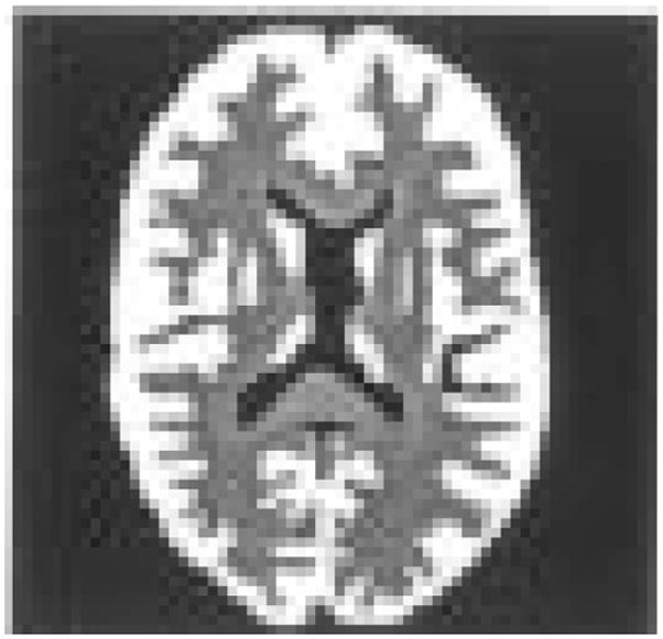
The slice from the Hoffman brain phantom used in this study.

The projection data, g, were computer generated with an analytical model of H that included the effects of attenuation and the finite resolution of a parallel-hole collimator. Blur was simulated for a collimator with a bore length of 34.0 mm and a bore diameter of 1.4 mm. The detector consisted of 643-mm pixels, and no other blur from the detector was assumed. Sixty-four projections were collected over 360°. In order to simulate the effects of modeling a continuous-to-discrete H with a discrete-to-discrete H, the projection data were generated using an H 5 × 5 times more finely sampled than the H used for the reconstruction. The finer sampling for generation of g was the only source of error for the H containing the system model with a 1.4–mm bore diameter. The incorrect H matrices used by the reconstruction algorithms were generated with imaging-system models that assumed bore diameters different than 1.4 mm. While it is probably unlikely in clinical practice that the assumed bore diameter for compensation is too large, results from overcompensation were included in order to illustrate the effects, positive or negative, if such an assumption was made.

III. Results

A. Qualitative Assessment With the Hoffman Brain Phantom

The slice from the digital Hoffman brain was projected through a simulated imaging system with a collimator of 1.4-mm bore diameter and 34.0-mm bore length. Statistical noise was added at 500 000 total projection counts. These data were then ML-EM reconstructed using H matrices that contained models assuming collimator blurs ranging from none to that resulting from a 2.0-mm bore diameter. Fig. 2 gives ML-EM estimates after 10, 20, 50, 100, 200, and 400 iterations reconstructed with an H matrix that assumed the correct 1.4-mm collimator bore diameter. The expected blurring at low iterations and noise buildup at higher iterations are seen. Fig. 3 gives estimates at the same iteration numbers for an H that assumed a perfect parallel-hole collimator (reconstruction with no compensation for detector blur, which we define as our most extreme undercompensation). Again, blurring at low iterations and increased noise at higher iterations is seen. The striking feature, however, when compared to Fig. 2, is the difference in noise texture between the images reconstructed with the two different collimator models. The noise in the uncompensated images seems to take on a much more salt-and-pepper character, with shorter apparent noise correlations than noise in the properly compensated images. Fig. 4 shows the estimates reconstructed with an H matrix that assumed a bore diameter of 2.0 mm (overcompensation). The noise correlations in these images appear to display even longer noise correlations than those in Fig. 2. Fig. 5 shows images after 200 iterations for H matrices assuming no collimator blur and blurs from collimator bore models ranging in size from 0.8 to 2.0 mm. It appears that, as the assumed collimator blur increases, so too does the length of the noise correlations (although Figs. 2–4 should be consulted when comparing models at a given iteration number as the apparent convergence is a function of the model). This is a counterintuitive result, as compensation for a broader point spread function should sharpen the image, and one might instinctively believe it would sharpen the noise as well [11].

Fig. 2.

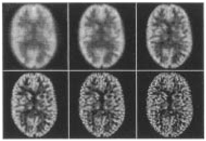
The reconstructed Hoffman brain phantom for correct compensation after 10, 20, 50, 100, 200, and 400 iterations.

Fig. 3.

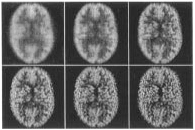
The reconstructed phantom with undercompensation (no blur modeled) after 10, 20, 50, 100, 200, and 400 iterations.

Fig. 4.

The reconstructed phantom for overcompensation (2.0-mm bore) after 10, 20, 50, 100, 200, and 400 iterations.

Fig. 5.

The Hoffman brain phantom after 200 iterations for no compensation and compensation assuming bore diameters of 0.8, 1.0, 1.2, 1.4, 1.6, 1.8, and 2.0 mm.

Although it is difficult to visually estimate in a quantitative manner the resolution of the images reconstructed using the different system models, there are no obvious differences in the resolution of the various images shown in Fig. 5. This is another counterintuitive result since, as we pointed out in Section I, for linear and shift-invariant systems the resolution and noise should follow the same course. With such an obvious differences in noise properties as are apparent in Figs. 2–5, we might expect an equally obvious difference in resolution, but it is difficult to say from visual analysis which of the images has the superior resolution.

B. Quantitative Assessment of Local Noise and Resolution Properties

The conclusions of Section III-A were based purely on qualitative visual analysis. In order to determine if these conclusions stood up to more quantitative inspection, we turned to the local noise and resolution methods discussed in Section II-B. For this study the uniformly emitting and attenuating disk served as the phantom.

The resolution was measured using a point source located 2.1 cm from the center of the disk. Noise-free projection data were generated for a collimator with a 1.4-mm bore diameter, and this noise-free data were ML_EM reconstructed using imaging-system models with assumed bore diameters of 0.8, 1.4, and 2.0 mm. The response to the point source was then Fourier transformed to generate the local MTF. Fig. 6 shows the MTF_r after 200 iterations for models assuming a bore diameter of 0.8, 1.4, and 2.0 mm, and Fig. 7 gives radially averaged profiles through the MTF_r of Fig. 6. It appears that the qualitative analysis of Section III-A was correct as no great differences in resolution are seen between the different compensations, though some differences at lower frequencies are seen.

Fig. 6.

The MTF_r for (from left to right) 0.8-, 1.4-, and 2.0-mm assumed bore diameter after 200 iterations for ML-EM reconstruction of a uniform disk.

Fig. 7.

Radially averaged profiles through the MTF_r for compensations at 0.8, 1.4, and 2.0 mm for ML-EM after 200 iterations.

Poisson statistical noise was added at a count level of 500 000 counts and the images were reconstructed using the ML-EM algorithm with the various correct and incorrect imaging-system models built into the H matrix. The local noise properties were estimated from a sample of 10 000 images reconstructed from independent Poisson noise realizations. The estimation procedure was performed using (6) with the expectation replaced by a sum over all the images.

C_r and W_r were calculated for r again located 2.1 cm from the center of the uniformly emitting disk and for compensation for collimators with bore diameters of 0.8, 1.4, and 2.0 mm. Images of the W_r are given in Fig. 8 and radially averaged profiles through the W_r are given in Fig. 9. Again, the qualitative analysis of Section III-A. appears to be correct. Figs. 8 and 9 show large differences in the noise correlations among the different compensations, with the correlation length increasing as the assumed bore diameter increases.

Fig. 8.

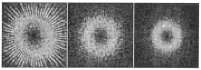
W_r for (from left to right) 0.8-, 1.4-, and 2.0-mm assumed bore diameters after 200 iterations for ML-EM reconstruction of a uniform disk.

Fig. 9.

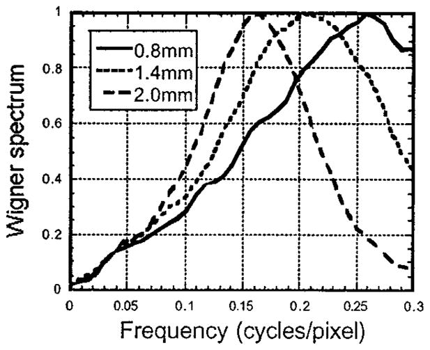
Radially averaged profiles through the W_r for compensations at 0.8, 1.4, and 2.0 mm for ML-EM.

Figs. 6–9 clearly demonstrate that the noise properties and resolution properties are changed in different manners when images are ML-EM reconstructed using different collimator-blur compensation models. In order to determine if it was the nonlinearity of ML-EM that led to the unexpected behavior in the ratio of noise correlations to resolution, we conducted the same experiment using the linear Landwebber algorithm. The results after 200 iterations are given in Fig. 10, which shows the radial average through the MTF_r for 0.8-, 1.4-, and 2.0-mm compensations, and Fig. 11, which gives the radial averages through the W_r for these same compensations. Figs. 10 and 11 show the same trends as were seen for ML-EM, with the noise correlations broader for overcompensated images but the resolution not changing greatly. We concluded from this that is was the shift-variant property of the reconstruction algorithms, rather than the nonlinearity, that lead to the different behaviors of the resolution and noise when the reconstruction model is altered.

Fig. 10.

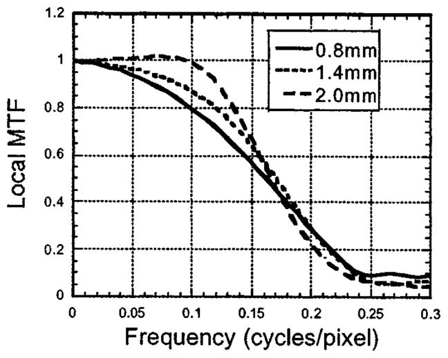
Radially averaged profiles through the MTF_r for compensations at 0.8, 1.4, and 2.0 mm after 200 Landweber iterations.

Fig. 11.

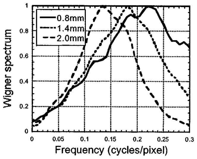
Radially averaged profiles through the W_r for compensations at 0.8, 1.4, and 2.0 mm after 200 Landweber iterations.

C. SNR in Terms of the Local NEQ

In Section I, we pointed out that for a linear and shift-invariant system the MTF and NPS change in a manner such that the ratio MTF²/NPS, termed the noise equivalent quanta (or NEQ), remains the same. For shift-variant tomographic images the NEQ is not precisely defined, but we can define a local NEQ (NEQ_r) as

$${\text{NEQ}}_{\mathbf{r}}(\mathit{\rho })={\text{MTF}}_{\mathbf{r}}^2(\mathit{\rho })/W_{\mathbf{r}}(\mathit{\rho }).$$ (8)

Fig. 12 gives the radial averages about r of 1-D profiles through the NEQ_r’s (200 iterations) for reconstruction models assuming collimator bore diameters of 0.8, 1.4, and 2.0 mm and r at 2.1 cm from the disk center. From the previous results, where we saw the noise power undergo large changes while the resolution remained relatively constant, we might expect large changes in the NEQ_r. However Fig. 12 shows very little change in NEQ_r. The differences at low frequencies are probably attributable to the fact that at a small radius there are fewer samples in the radial averaging, and hence greater estimation error for the W_r.

Fig. 12.

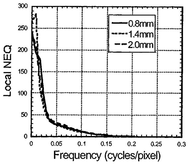
Radially averaged profiles through the NEQ_r for compensations at 0.8 mm, 1.4 mm, and 2.0 mm for ML-EM.

In order to determine how the W_r could change so dramatically while the NEQ_r remained constant, we plotted the natural log of the NEQ_r (Fig. 13). Like Fig. 12, this shows that the NEQ_r is unchanged at lower frequencies. However Fig. 13 shows large changes in NEQ_r at higher frequencies—the frequencies where the noise correlations differ the most between the levels of compensation. At these frequencies, though, the NEQ_r is so small that the differences do not show up on a linear plot, and the overall signal to noise for the image is likely unaffected by these differences.

Fig. 13.

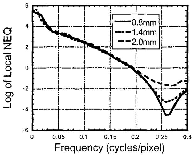
The log values for the NEQ_r’s plotted in Fig. 12.

While the overall NEQ_r is little affected, it should be pointed out that an ideal-observer model such as the NEQ_r is able to perfectly distinguish a given frequency while the human observer is not. Noise correlations at frequencies containing little signal could well have a large effect on human task performance. The fact that the NEQ_r remains unchanged regardless of compensation does not necessarily imply that the large changes in W_r are not important to human task performance.

IV. Conclusion

We have studied the effects of incorrect compensation for detector blur on the noise and resolution properties of ML-EM images. Using local noise and resolution measures, we have demonstrated that the noise properties are greatly changed by the model while the resolution properties are less affected. One interesting result is that the noise correlations are actually broadened as the blur is more compensated for, with the noise for highly-compensated images clumped at fewer and lower frequencies.

Despite these large differences in the W_r, studies involving the NEQ_r revealed little difference in SNRs for overcompensated, undercompensated, or properly compensated images. The only differences seen were at values so low that a log plot was required in order to see them.

While the ideal observer has no difficulty with noise at frequencies where the signal is low, the human observer might not find it such an easy task to ignore noise at frequencies without signal. More analysis is required in order to ascertain the impact of these findings on the quality of reconstructed images. The differences in W_r were surprising, and it is important to determine if this has an effect on image quality in terms of the ability of a human to perform a task. Methods we shall pursue for studying these effects involve more quantitative measures of image quality in terms of human task performance. These include human observer studies and studies using computer observers whose performance well models that of the human observer.

References

- 1.Liang Z, Turkington TG, Gilland DR, Jaszczak RJ, Coleman RE. Simultaneous compensation for attenuation, scatter and detector response for SPECT reconstruction in 3 dimensions. Phys Med Biol. 1992;37:587–603. doi: 10.1088/0031-9155/37/3/007. [DOI] [PubMed] [Google Scholar]
- 2.Wilson DW, Tsui BMW. Noise properties of filtered backprojection and ML-EM reconstructed emission tomographic images. IEEE Trans Nucl Sci. 1993;40:1198–1203. [Google Scholar]
- 3.Tsui BMW, Frey EC, Zhao X, Lalush DS, Johnston RE, McCartney WH. The importance and implementation of accurate 3D compensation methods for quantitative SPECT. Phys Med Biol. 1994 Mar;39:509–530. doi: 10.1088/0031-9155/39/3/015. [DOI] [PubMed] [Google Scholar]
- 4.Wigner EP. On the quantum correction for thermo-dynamic equilibrium. Phys Rev. 1933;40:749–759. [Google Scholar]
- 5.Shepp LA, Vardi Y. Maximum likelihood reconstruction for emission tomography. IEEE Trans Med Imaging. 1982;MI-1:113–122. doi: 10.1109/TMI.1982.4307558. [DOI] [PubMed] [Google Scholar]
- 6.Wilson DW, Tsui BMW. Spatial resolution properties of FB and ML-EM reconstructed images. Conf Rec IEEE Nuclear Science Symp. 1994:1189–1193. [Google Scholar]
- 7.Frieden BR. The importance of being positive. Proc SPIE. 1981;292:151–159. [Google Scholar]
- 8.Fessler JA, Rogers WL. Spatial resolution properties of penalized-likelihood image reconstruction: Space-invariant tomographs. IEEE Trans Med Imaging. 1996;5:1346–1358. doi: 10.1109/83.535846. [DOI] [PubMed] [Google Scholar]
- 9.Wilson DW. PhD dissertation. Univ. North Carolina; Chapel Hill: 1994. Noise and resolution properties of FB and ML-EM reconstructed SPECT images. [Google Scholar]
- 10.Hoffman EJ, Cutler PD, Digby WM, Mazziotta JC. 3-D phantom to simulate cerebral blood flow and metabolic images for PET. IEEE Trans Nuclear Sci. 1990;37:616–620. [Google Scholar]
- 11.Byrne CL. Iterative image reconstruction algorithms based on cross-entropy minimization. IEEE Trans Image Processing. 1993;2:96–103. doi: 10.1109/83.210869. [DOI] [PubMed] [Google Scholar]