Lévy fluctuations and mixing in dilute suspensions of algae and bacteria

Abstract

Swimming micro-organisms rely on effective mixing strategies to achieve efficient nutrient influx. Recent experiments, probing the mixing capability of unicellular biflagellates, revealed that passive tracer particles exhibit anomalous non-Gaussian diffusion when immersed in a dilute suspension of self-motile Chlamydomonas reinhardtii algae. Qualitatively, this observation can be explained by the fact that the algae induce a fluid flow that may occasionally accelerate the colloidal tracers to relatively large velocities. A satisfactory quantitative theory of enhanced mixing in dilute active suspensions, however, is lacking at present. In particular, it is unclear how non-Gaussian signatures in the tracers' position distribution are linked to the self-propulsion mechanism of a micro-organism. Here, we develop a systematic theoretical description of anomalous tracer diffusion in active suspensions, based on a simplified tracer-swimmer interaction model that captures the typical distance scaling of a microswimmer's flow field. We show that the experimentally observed non-Gaussian tails are generic and arise owing to a combination of truncated Lévy statistics for the velocity field and algebraically decaying time correlations in the fluid. Our analytical considerations are illustrated through extensive simulations, implemented on graphics processing units to achieve the large sample sizes required for analysing the tails of the tracer distributions.

1. Introduction

Brownian motion presents one of the most beautiful manifestations of the central limit theorem in Nature [1]. Reported as early as 1784 by the Dutch scientist Jan van Ingen-Housz [2], the seemingly unspectacular random motion of mesoscopic particles in a liquid environment made an unforeseeable impact when Perrin's seminal experiments of 1909 [3] yielded convincing evidence for the atomistic structure of liquids. This major progress in our understanding of non-living matter—which happened long before direct observations of atoms and molecules came within experimental reach—would not have been possible without the works of Sutherland [4] and Einstein [5], who were able to link the microscopic properties of liquids to a macroscopic observable, namely the mean square displacement (MSD) of a colloidal test particle.

Caused by many quasi-independent random collisions with surrounding molecules, Brownian motion in a passive liquid is quintessentially Gaussian, as predicted by the central limit theorem. Remarkably, however, recent experiments by Leptos et al. [6] revealed notable non-Gaussian features in the probability distribution of a tracer particle, when a small concentration of microscale swimmers, in their case unicellular biflagellate Chlamydomonas reinhardtii algae, was added to the fluid. Understanding this apparent violation of the central limit theorem presents a challenging unsolved problem, whose solution promises new insights into the mixing strategies of micro-organisms [7]. Here, we shall combine extensive analytical and large-scale numerical calculations to elucidate the intimate connection between the flow field of an individual micro-organism and the anomalous (non-Gaussian) diffusion of tracer particles in a dilute swimmer suspension.

Modern high-speed microscopy techniques resolve the stochastic dynamics of micron-sized tracer particles to an ever increasing accuracy [8,9]. This opens the exciting possibility of using high-precision tracking experiments to probe the statistics of the flow fields created by active swimmers, and hence their connection to physical properties and evolutionary strategies of micro-organisms that live in liquid environments [6,10,11]. Furthermore, a novel class of micromechanical devices [12,13] uses non-equilibrium fluctuations generated by bacteria as a fundamental ingredient of their operation. To explain and exploit the non-equilibrium conditions in active suspensions, it is important to fully understand the relation between the experimentally observed features of tracer displacements and the characteristics (such as self-propulsion mechanisms) of the algae or bacteria.

The observations of Leptos et al. [6] demonstrate that the time-dependent probability distributions of tracer displacements in dilute algae suspensions exhibit tails that decay much more slowly than would be expected if the tracers obeyed purely Gaussian statistics. At high swimmer concentrations, enhanced transport might be expected [14–17], as collective behaviour emerges from swimmer interactions, which can lead to the formation of large-scale vortices and jets. In dilute suspensions, however, where swimmer–swimmer interactions can be neglected, a satisfactory quantitative understanding of the underlying velocity statistics is still lacking. Below, we are going to show that the velocity distribution produced by the swimmers takes a tempered (or regularized) Lévy form [18,19], and that the long-time behaviour of the tracers' positional probability distribution function can be understood in terms of correlated truncated Lévy flights [20]. In a dilute suspension of swimmers, the fundamental ingredient of such anomalous behaviour is an ultraslow convergence of the central limit theorem. This is different from tracers that undergo non-Gaussian diffusion in other complex systems, like colloidal gels [21] or granular gases [22], where spatio-temporal correlations are predominant.

If a microswimmer is self-propelled, with no external forces acting, its flow field scales with distance as r⁻ⁿ for an exponent n ≥ 2 [23]. We will demonstrate that it is this form of the power-law decay that is responsible for the anomalous diffusion of tracer particles [6]. Remarkably, qualitatively different behaviour can be expected in suspensions of sedimenting swimmers: if gravity plays an important role for the swimmer dynamics, the far-field flow decays as r⁻¹ and tracers will diffuse normally. Finally, our results suggest that, on sufficiently long times scales, anomalous tracer diffusion in dilute active suspensions can be viewed as a natural example of a stochastic process described by a fractional diffusion equation.

2. Model

Given an advecting flow u_N(t,r), generated by a dilute suspension of N self-swimming micro-organisms, we model the dynamics x(t) of a passive, colloidal tracer particle (radius a) by an overdamped Langevin equation of the form:

2.1

The random function ξ(t) = (ξ_i(t))_i=1,2,3 represents uncorrelated Gaussian white noise with 〈ξ_i(t)〉 = 0 and 〈ξ_i(t)ξ_j(t′)〉 = δ_ijδ(t − t′), describing stochastic collisions between the tracer and the surrounding liquid molecules. The thermal diffusion coefficient D₀ in a fluid of viscosity η is determined by the Stokes–Einstein relation D₀ = k_BT/(6πηa).

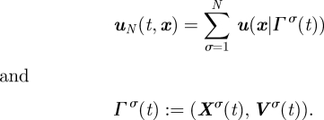
If the Reynolds number is very small, the net flow owing to σ = 1, …, N active swimmers, located at positions X^σ(t) and moving at velocity V^σ(t), is, in good approximation, the sum of their individual flow fields u,

2.2

As we are interested in physical conditions similar to those in the experiments of Leptos et al. [6], our analysis will focus on a dilute suspension of active particles, corresponding to the limit of a small volume filling fraction ϕ ≪ 1. In this case, binary encounters between swimmers are negligible perturbations. Moreover, we can ignore random reorientation of swimmers caused by rotational diffusion (owing to thermal fluctuations) and search behaviour (like chemotaxis or phototaxis), since these effects take place on the order of several seconds and thus are not relevant to the tracer dynamics. Indeed, in dilute homogeneous solutions, it is irrelevant for the tracer statistics (even on longer time scales) whether a tracer experiences two successive scatterings from the same tumbling swimmer or from two different non-tumbling swimmers. It is therefore sufficient to assume that each swimmer moves ballistically,

2.3

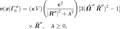
For dilute suspensions, the initial swimmer coordinates Γ^σ(0) = (X₀^σ,V₀^σ) are independent and identically distributed random variables with one-particle probability density function (PDF) Φ₁(Γ₀^σ). More specifically, we assume that the distribution of the initial positions X₀^σ is spatially uniform and that the swimmers have approximately the same speed V, that is Φ₁(Γ₀^σ) ∝ δ(V − |V₀^σ|). To complete the definition of the model, we need to specify the flow field u(x|Γ^σ(t)) generated by a single swimmer. There are various strategies for achieving directed propulsion at the microscale [24]. Small organisms, like algae and bacteria, can swim by moving their slender filaments in a manner not the same under time reversal. Self-motile colloids, a class of miniature artificial swimmers, are powered with interfacial forces induced from the environment [25]. Although both of these are active particles, microscopic details of their geometry and self-propulsion can lead to different velocity fields. This, in turn, affects how a tracer migrates in their flow. In the Stokes regime, if external forces are absent, self-propelled particles or micro-organisms generate velocity fields decaying as r⁻² or faster  [23,25]. As we are interested in the general features of mixing by active suspensions, and there is no universal description of the flow around an active object, it is helpful to consider simplified velocity field models that capture generic features of real microflows.

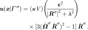
We shall focus on two simplified models (figure 1) that can be interpreted as contributions in a general multipole expansion of a flow field. Specifically, we will compare a co-oriented toy model [26] with a trivial angular dependence

2.4a

to a more realistic dipolar (or stresslet) flow field [27]

2.4b

Figure 1.

Flow fields of the model swimmers considered in our analytical and numerical calculations. In both plots, the swimmer is oriented upwards and the flow is normalized by the swimming speed. The arrows indicate velocity direction and the colours represent magnitude. (a) Co-oriented model with r⁻² decay and (b) stroke-averaged flow generated by a dipolar ‘pusher’. Parameters are those of figure 2.

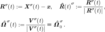
In equations (2.4a,b), the vector R^σ(t) := X^σ(t) − x connects the swimmer and tracer position at time t, is the associated unit vector, and defines the swimmer's orientation and swimming direction. The parameter ε characterizes the swimmer length scale, κ is a dimensionless constant that relates the amplitude of the flow field to the swimmer speed and λ regularizes the singularity of the flow field at small distances. The co-oriented ‘toy model’ (2.4a), owing to its minimal angular dependence, is useful for pinpointing how the tracer statistics depend on the distance scaling of the flow field. For n = 1, the scaling is equivalent to that of an ‘active’ colloid or forced swimmer, whereas for n ≥ 2, the scaling resembles that of various natural swimmers not subjected to an external force. In particular, the case n = 2 allows us to ascertain the effects of the angular dependence of the flow-field structure on tracer diffusion, by comparing against the more realistic dipolar model (C 1). The latter is commonly considered as a simple stroke-averaged description for natural microswimmers [28,29]. As shown in Dunkel et al. [26], stroke-averaged models are able to capture the most important aspects of the tracer dynamics on time scales longer than the swimming stroke of a micro-organism.

3. Results

We are interested in computing experimentally accessible, statistical properties of the tracer particles, such as their velocity PDF, correlation functions and position PDF. These quantities are obtained by averaging suitably defined functions with respect to the N-swimmer distribution Φ_N = Π_σΦ₁(Γ₀^σ). A detailed description of the averaging procedure and a number of exact analytical results are given in the appendices, below we shall restrict ourselves to discussing the main results and their implications.

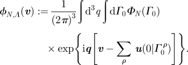
We begin by considering the equal-time velocity PDF and velocity autocorrelation function at a fixed point in the fluid. As we are primarily interested in the swimmer contributions, we will focus on the deterministic limit D₀ = 0 first. The additive effect of thermal Brownian motion will be taken into account later, when we discuss the position statistics of the tracer. Considering a suspension of N swimmers, confined by a spherical volume of radius Λ, the equal-time velocity PDF ϕ_N,Λ(v) and velocity autocorrelation function C_N,Λ(t) of the flow field near the centre of the container are formally defined by

3.1a

and

3.1b

where the average 〈 · 〉 is taken with respect to the spatially uniform initial distribution of the swimmers. For the models (2.4a,b), it is possible to determine ϕ_N,Λ and C_N,Λ analytically.

3.1. Velocity probability density function: slow convergence of the central limit theorem for n ≥ 2

To elucidate the origin of the unusual velocity statistics in an active suspension, let us consider the tracer velocity PDF when there is a single swimmer present, ϕ_1,Λ(v). The tail of this function reflects large tracer velocities generated by close encounters with the swimmer. It is instructive to start with the (unphysical) limit λ = 0, where the interaction diverges at short distances and there is no cut-off for large velocities. In this case, one readily finds from equation (A 5a) that asymptotically ϕ_1,Λ(0,v) ∝ |v|^−(3+3/n). This means that the variance of the probability distribution is finite for n = 1, but infinite for n ≥ 2. According to equation (2.2), the flow field owing to N swimmers is the sum of N independent and identically distributed random variables. Hence, the central limit theorem predicts that, for λ = 0 and n = 1, the velocity distribution ϕ_N,Λ converges to a Gaussian in the large N limit, whereas for λ = 0 and n ≥ 2 one expects non-Gaussian behaviour owing to the infinite variance of ϕ_1,Λ.

For a real swimmer, the flow field is strongly increasing in the vicinity of the swimmer [23,30], but remains finite owing to lubrication effects and non-zero swimmer size. This corresponds in our model to a positive value of λ. For λ > 0, the variance of the one-swimmer PDF ϕ_1,Λ remains finite and, formally, the conditions for the central limit theorem are satisfied for all n ≥ 1. However, for n ≥ 2, the variance of ϕ_1,Λ remains very large and the convergence to a Gaussian limiting distribution is very slow. Our subsequent analysis demonstrates that the velocity PDF is more accurately described by a tempered Lévy-type distribution.

These statements are illustrated in figure 2, which shows velocity PDFs obtained numerically (symbols) and from analytical approximations (solid curves) for the co-oriented model with n = 1 (figure 2a) and n = 2 (figure 2b), and the dipolar model (figure 2c) at different swimmer volume fractions φ := N(ε/Λ)³. As evident from figure 2a, for n = 1, the velocity PDF indeed converges rapidly to the Gaussian shape, in accordance with the central limit theorem. By contrast, for velocity fields decaying as r⁻ⁿ with n ≥ 2, the convergence is surprisingly slow and one observes strongly non-Gaussian features at small filling fractions φ. The arrows highlight this regime, which shows a power-law dependence of the velocity distribution on the magnitude of the velocity, a signature of a Lévy distribution.

Figure 2.

Velocity probability density function (PDF) of a tracer particle in the flow generated by different concentrations of swimmers. The solid curves are based on approximation (3.3), using the exact second and fourth moments of the velocity PDFs, as shown in the appendices. (a) For the co-oriented model (2.4) with long-range hydrodynamics n = 1, the velocity PDFs from simulations (symbols) converge rapidly to the Gaussian distribution predicted by the central limit theorem (solid curves), even at low volume fractions φ ≃ 0.4%. (b) By contrast, for the co-oriented model with n = 2, the central limit theorem convergence is very slow and the velocity distribution exhibits strongly non-Gaussian features at volume fractions similar to those realized by recent experiments [6]. (c) The velocity PDF for the dipolar swimmer model looks very similar to that of our co-oriented model (b), which means the angular dependence does not play an important role for the velocity distribution. Simulation parameters are κ = 0.4875, V = 50 µm s⁻¹, and ε = 5 µm. The sample size is 4 × 10⁶ throughout. Red circles or solid line, ϕ = 0.4%; orange squares or solid line, ϕ = 0.8%; green triangles or solid line, ϕ = 1.6%; cyan inverted traingles or solid line, ϕ = 3.2%. In figure 7, the one-dimensional data of (a) and (b) are displayed as a semilog plot.

The remarkably slow convergence to the Gaussian central limit theorem prediction can be understood quantitatively by considering the characteristic function

3.2

of the velocity PDF (A 5a). A detailed analytical calculation (see the appendices) shows that the exact result for χ_ϕ(q) can be approximated by

3.3

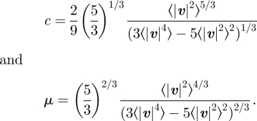
The coefficients c and μ are explicitly given by equation (B 19c) for the co-oriented model or by using equation (C 7) for the dipolar model. The probability distribution , which reduces to a Gaussian for α = 2, is of the tempered Lévy form, and gives rise to the following tracer velocity moments

3.4a

and

3.4b

By studying asymptotic behaviour in the small cut-off limit λ → 0 one finds that, for velocity fields u decaying as r⁻ⁿ,

3.5

This result confirms that for colloidal-type interactions with n = 1 the velocity PDF is Gaussian, whereas for n ≥ 2 deviations from Gaussianity occur in agreement with our numerical results of figure 2. In the limit μ = 0, equation (3.3) describes the family of Lévy stable distributions. These distributions arise from a generalized central limit theorem [31] relevant to random variables having an infinite variance. Specifically for n = 2, one recovers the Holtsmark distribution that describes the statistics of the gravitational force acting on a star in a cluster [32] and of the velocity field created by point vortices in turbulent flows [33]. These examples both consider fluctuations that occur owing to interactions decaying as r⁻² in three dimensions, which lead to a Lévy stable distribution with α = 3/2 (neglecting regularization). In such a case, the probability distributions for each component v_i are not independent as does not factorize. Nevertheless, the marginal probability distribution that results from integrating over the other dimensions is a Lévy stable distribution with the same α. A different situation occurs in one dimension as a power-law distribution that falls off like v⁻ⁿ has a divergent variance for any n. This is the case for single molecules that undergo sudden jumps [34,35], which are well-described by Lévy statistics even if n = 1.

However, for realistic non-singular flow fields, corresponding to finite values of λ, we generally have μ > 0. Specifically, by matching the exact velocity moments to those in equation (A 11), one finds that for the co-oriented model (2.4a) with n = 1

3.6

at leading order in ℓ := λ/Λ, whereas for n = 2

3.7a

and

3.7b

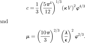
For the dipolar model (C 1), one obtains the same scaling of (c,μ) with (ϕ,λ) as in equation (B 19d) but with a slightly different numerical prefactor, yielding in the small cut-off limit λ → 0

3.8a

and

3.8b

Note that equation (3.6) suggests for colloidal-type flow fields with u ∝ r⁻¹, the appropriate thermodynamic limit is given by N,Λ → ∞ such that N/Λ² = const., whereas we must fix φ = const. if u ∝ r⁻ⁿ, n ≥ 2. Furthermore, equations (3.7b) and (3.8a) imply that μ → 0 and 〈|v|²〉 → ∞ for a vanishing regularization parameter λ → 0. This illustrates that Lévy-type behaviour becomes more prominent, the more ‘singular’ the velocity field in the vicinity of the swimmer.

The solid curves in figure 2 are based on approximation (3.3), using the exact second and fourth moments of the velocity PDFs, as given in the appendices. For u ∝ r⁻², the Gaussian prediction of the central limit theorem becomes accurate only at large volume fractions (φ > 25%). In the dilute regime φ ≪ 1, the bulk of the probability comes from a Lévy stable distribution before it crosses over to quasi-Gaussian decay, reflected by the (truncated) power-law tails in figure 2b,c. We may thus conclude that the fluid velocity in a dilute swimmer suspension is a biophysical realization of truncated Lévy-type random variables [20].

3.2. Flow-field autocorrelation

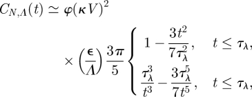
The similarity of figure 2b,c suggests that the angular flow-field structure is not important for the equal-time velocity distribution. By contrast, the velocity autocorrelation function C_N,Λ(t) depends sensitively on the angular details, as illustrated in figure 3. For both our co-oriented model (2.4a) with n = 1,2 and the dipolar model (C 1), the function C_N,Λ(t) can be determined analytically (see the appendices). From the exact results, one finds that for n = 2 in the thermodynamic limit at long times t ≫ τ_ε := ε/V

3.9

Figure 3.

Owing to the different flow topologies, the velocity autocorrelation function for dipolar swimmers (C 1) decays faster than that for the co-oriented model (2.4a) with n = 2. Solid curves indicate the exact analytical solution and symbols correspond to simulation data. Dotted and dashed curves illustrate, respectively, the long-time approximation and its behaviour in the thermodynamic limit. Parameters are those of figure 2. Red circles or solid line, dipolar model, exact; red dashed line, dipolar model, equation (3.10a); red dotted line, dipolar model, equation (3.10b); orange squares or solid line, co-oriented model, exact.

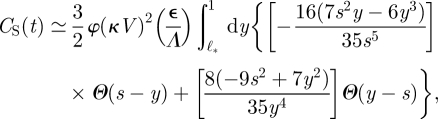
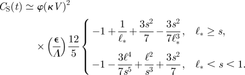
For comparison, the velocity autocorrelation function for dipolar swimmers can be approximated by

3.10a

where ℓ_* := 4ℓ/π and s := tV/Λ < 1. The approximation (C 16), shown as the dotted line in figure 3, becomes exact at long times. In the thermodynamic limit, it reduces to

3.10b

where τ_λ := 4λ/(πV). Note that equation (C 18) predicts an asymptotic t⁻³ decay, which is considerably faster than the t⁻¹ decay for the co-oriented model, cf. equation (B 29c). This is due to the different angular structure of their respective flow fields. The excellent agreement between simulation data and the exact analytic curves (solid) in figure 3 also confirms the validity of our simulation scheme (see numerical methods in appendix D).

3.3. Mean square displacement

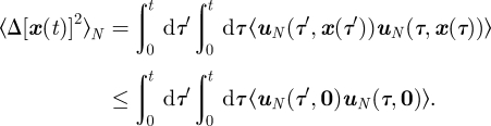
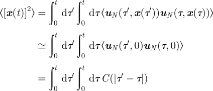
Having discussed the velocity statistics, we next analyse the tracer displacements. To that end, we will focus on the practically more relevant dipolar swimmer case, and include the effects of thermal Brownian motion (so D₀ > 0). A first quantifier, that can be directly measured in experiments, is the MSD 〈Δ[x(t)]²〉 ≃ 〈Δ[x(t)]²〉_N + 6D₀t. Assuming spatial homogeneity and spatially decaying correlations, the velocity autocorrelation function can be used to obtain an upper bound for the swimmer contribution

3.11

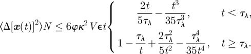
Inserting the approximate result (C 18), we find

3.12

Equation (3.12) implies that tracer diffusion owing to the presence of dipolar swimmers is ballistic at short times t ≪ τ_λ and normal at large times t ≫ τ_λ (figure 4). Qualitatively, the predicted linear growth 〈Δ[x(t)]²〉 ∝ t agrees with the experimental results of Leptos et al. [6]. Generally, the asymptotic diffusion constant will be of the form D ≃ D₀ + νφκ²Vε, where ν is a numerical prefactor of order unity that encodes spatial correlations neglected in equation (3.11).

Figure 4.

Mean square displacement at different volume fractions. Solid lines are analytical upper bounds, 6(D₀ + ϕκ² Vε)t ≥〈Δ[x(t)]²〉, and symbols display the ensemble average from simulations. Parameters are those of figure 2. Red circles or solid line, ϕ = 0.0%; orange squares or solid line, ϕ = 0.4%; green triangles or solid line, ϕ = 0.8%; cyan inverted triangles or solid line, ϕ = 1.6%.

3.4. Evolution of the position probability density function

The spatial motion of a passive tracer in a fluctuating flow u(t,r) is described by the position PDF P(t,r) = 〈δ(r − x(t))〉. For Gaussian fields, uniquely defined by the two-point correlation function 〈u_i(t,r)u_j(t′,r′)〉, it is possible to characterize P(t,r) analytically for some classes of trajectories x(t) [36]. However, our analysis above indicates that the statistics in an active suspension are neither δ-correlated nor Gaussian, exhibiting features of Lévy processes.

Generally, the hierarchy of correlations in Lévy random fields is poorly understood [37]. It is therefore unclear how to adapt successful models of random advection by a Gaussian field [38] or, more generally, extend the understanding of coloured Gaussian noise [36] to coloured Lévy processes. These theoretical challenges make it very difficult, if not impossible, to construct an effective diffusion model that bridges the dynamics of P(t,r) on all of the time scales. Partial theoretical insight can be gained, however, by considering the asymptotic short- and long-time behaviour.

At short times t ≪ τ_λ, the position PDF combines ballistic transport from constant swimmer advection and diffusive spreading from thermal Brownian effects. For experimentally relevant parameters [6], normal diffusion is much stronger than the advection and, at these times, the dynamics of P(t,r) are captured by the normal diffusion equation. If Brownian motion is neglected, we have P(t,r) = t⁻³ϕ_N,Λ(r/t) with ϕ_N,Λ(v) as the tempered Lévy velocity PDF. The resulting ‘ballistic’ Lévy distribution is in good agreement with simulation data for D₀ = 0 at short times, see inset of figure 5a.

Figure 5.

Radial position PDF of a tracer in a dilute suspension of dipolar swimmers at various times. Solid curves represent analytical forms of P(t,r) and symbols illustrate histograms determined from simulations. Insets (b) and (c) show the same quantities on a log–log scale. Volume fractions and symbols are those of figure 4. Parameters are those of figure 2 with D₀ = 0.245 µm²s⁻¹. (a) Short-time regime. At these times, Brownian motion effectively dominates constant advection for our choice of parameters. In the limit of no thermal noise (inset), the position PDF is the tempered Lévy velocity PDF ϕ_N,Λ(v) after a rescaling with t. (b) Transient behaviour. This period corresponds to an intermediate decay of the velocity autocorrelation. (c) Asymptotic long-time regime. Eventually, random advection from many low Reynolds number swimmers becomes equivalent to a tempered Lévy flight. The solution to the fractional diffusion equation (3.14) is matched against simulations by fitting its coefficients D_α and K, see also figure 6.

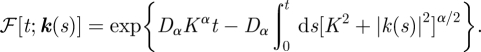
For long times t ≫ τ_λ, after the correlations of the velocity field have vanished (typically after several seconds), we may interpret a tracer diffusing in an active suspension as a realization of an uncorrelated tempered Lévy process. Effectively, this corresponds to replacing u_N(t,r) from equation (A 1) with a δ-correlated but non-Gaussian random function ζ(t). To characterize the statistical properties of the swimmer-induced noise ζ(t), we need to specify its characteristic functional ℱ[t;k(s)] [39]. Our earlier findings, that the asymptotic MSD grows linearly in time and that the velocity field amplitudes follow a tempered Lévy stable distribution, suggest the functional form:

3.13

Here, D_α is an anomalous diffusion coefficient of dimensions m^αs⁻¹ and the regularization parameter K has dimensions m⁻¹. For α = 2, ζ(t) reduces to Gaussian white noise. Note we may also derive the functional ℱ[t;k(s)] under the assumption that ζ(t) consists of independent increments with the equal-time distribution from equation (3.3). Using a standard procedure outlined in Budini & Cáceres [40], the Fokker–Planck equation corresponding to equation (3.13) is found to be

3.14

where we also included the contribution from normal diffusion. In Fourier space, the solution of equation (3.14) reads

3.15

Using a Levenberg–Marquardt algorithm that numerically evaluates the inverse Fourier transform, we fit the coefficients D_α and K to the data from our simulations. Equation (3.15) compares well against the long-time data in figures 5c and 6, especially in the asymptotic regime. It is worth emphasizing that, although the motion of the tracers at long times is non-Gaussian and described by a fractional diffusion equation, the asymptotic MSD exhibits normal growth, 〈Δ[x(t)]²〉 ∝ t.

Figure 6.

Time evolution of the marginal position PDF at a volume fraction ϕ = 1.6%. Solid curves represent equation (3.15) with fitted coefficients (shown only at long times) and symbols illustrate histograms determined from simulations. Simulation parameters are those of figure 2 with D₀ = 0.245 µm² s⁻¹. Fit parameters are α = 3/2, D_α = 0.253 µm^α s⁻¹, and K = 0.0825 µm⁻¹. Red circles, t = 1 s; orange squares, t = 5 s; green triangles, t = 25 s; cyan inverted triangles or solid line, t = 50 s; purple diamonds or solid line, t = 100 s. At intermediate times t ≃ 1 s, our data resemble the measurements from Leptos et al. [6].

On intermediate time scales, when the velocity autocorrelations are already decaying, but still non-negligible owing to their t⁻³ scaling (figure 3), the transient behaviour of the position PDF can interpreted as a superposition of two distinct components: (i) Quasi-ballistic tracer displacements, which are remnants of the short-time dynamics and may dominate the tails of the tracer position distribution, and (ii) fractional diffusive behaviour owing to the onset of tracer scattering by multiple swimmers. A quantitative comparison suggests that the measurements of tracer diffusion in Chlamydomonas suspensions by Leptos et al. [6], who focused on the range t ≲ 2 s, are exploring this intermediate regime.

4. Conclusions

Understanding the mixing and swimming strategies of algae and bacteria is essential for deciphering the driving factors behind evolution from unicellular to multicellular life [10]. Recent experiments on tracer diffusion in dilute suspensions of unicellular biflagellate C. reinhardtii algae [6] have shown that micro-organisms are able to significantly alter the flow statistics of the surrounding fluid, which may result in anomalous (non-Gaussian) diffusive transport of nutrients throughout the flow.

Here, we have developed a systematic theoretical description of anomalous tracer diffusion in dilute, active suspension. We demonstrated analytically and by means of simulations on a graphics processing unit (GPU) that, depending on the distance scaling of microflows, qualitatively different flow-field statistics can be expected. For colloidal-type flow fields that scale as r⁻¹ (owing to the presence of an external force), the local velocity fluctuations in the fluid are predominantly Gaussian even at very small volume filling fraction, as expected from the classical central limit theorem. By contrast, flow fields that rise as r⁻² or faster in the vicinity of the swimmer will exhibit Lévy signatures. Very recent measurements by Rushkin et al. [41] appear to confirm this prediction. When the statistics are non-Gaussian, our results show that the asymptotic convergence properties of velocity fluctuations in active swimmer suspensions are well-approximated by truncated Lévy random variables [20]. Though we prepared data for swimmers that are ‘pullers’ (κ < 0), these statements are also true for ‘pushers’ (κ > 0) as long as the suspension remains statistically homogeneous and isotropic.

With regard to experimental measurements, it is important to note that the tracer velocity is a well-defined observable only if thermal Brownian is negligible (corresponding to the limit D₀ = 0). Otherwise, the associated displacements over a time-interval Δt contain a component that scales as . This fact must be taken into account, when one attempts to reconstruct velocity distributions from discretized trajectories: if thermal Brownian motion is a relevant contribution in the tracer dynamics, the measured distributions will vary depending on the choice of the discretization interval.

Our analysis further illustrates that, for homogeneous suspensions, the angular shape of the swimmer flow field is not important for the local velocity distribution, which is dominated by the radial flow structure. By contrast, the temporal decay of the velocity correlations sensitively depends on the angular topology of the individual swimmer flow fields. Specifically, our analytical calculations predict that velocity autocorrelations in a dipolar swimmer suspension vanish algebraically as t⁻³. This prediction could, in principle, be tested experimentally by monitoring the flow field at a fixed point in the fluid, using a set-up similar to that in Rushkin et al. [41].

Finally, we propose that the asymptotic tracer dynamics can be approximated by a fractional diffusion equation with linearly growing asymptotic MSD. If the swimmers also undergo directional changes (owing to stimuli response or thermal fluctuations), the net result will only be a further decorrelation of the velocity fluctuations (assuming the suspension remains homogeneous and isotropic). In such a case, the tempered Lévy PDF predicted by equation (3.14) should become valid at earlier times. It would be interesting to learn whether the fractional evolution of the tracer position distributions at long times can be confirmed experimentally. This, however, will require observational time spans that go substantially beyond those considered in Leptos et al. [6].

In conclusion, the correct and complete interpretation of experimental data requires an extension of Brownian motion beyond the currently existing approaches [18,19,36]. Although many challenging questions remain—in particular, regarding the consistent formulation of a generalized diffusion theory that combines Lévy-type fluctuations with time correlations—we hope that the present work provides a first step towards a better understanding of present and future experiments.

Appendix A. Summary of model assumptions

A.1. Tracer dynamics

We consider the three-dimensional motion x(t) = (x_i(t)) of a passive tracer particle in a fluid that contains σ = 1, …, N active particles (such as algae or bacteria), which are described by phase space coordinates . We assume that, in good approximation, the tracer particle does not affect the swimmers, so that Γ(t) is approximately independent of x(t). Neglecting Brownian motion effects (corresponding to D₀ = 0 in equation (2.1) of the main text), the tracer motion can be described by the overdamped equation (low Reynolds number or Stokes regime)

A 1

Here, u_N denotes the velocity field generated by N swimmers and u(x|Γ^σ) the contribution of an individual swimmer σ to the fluid flow at position x. In appendix §§B and C below, we shall study two different models for u(x|Γ^σ).

A.2. Swimmer dynamics and statistics

We restrict our considerations to the dilute limit of small swimmer concentrations. In this case, we may assume that the swimmers move approximately on straight lines at constant velocity . Then, Γ^σ(t) is uniquely determined by its initial condition Γ₀^σ := Γ^σ(0) = (X₀^σ,V₀^σ), and we have

A 2

Throughout, it is assumed that the swimmer speed is roughly the same and equal to V and that, initially, the swimmers are uniformly distributed in a large spherical container (radius Λ), i.e. the initial conditions Γ₀^σ = (X₀^σ,V₀^σ) are i.i.d. random variables with joint PDF

A 3

where is the indicator function of the spherical container volume ,

A 4

We are interested in the velocity distribution at the centre of the volume, formally defined by

A 5a

and, moreover, in the flow-field autocorrelation function at a fixed point in the fluid far from the boundaries,

A 5b

where 〈 · 〉 indicates an average with respect to the initial swimmer distribution (A 3). Generally, we are interested in evaluating these quantities in some suitably defined thermodynamic limit N, Λ → ∞.

A.3. Characteristic function

Consider the characteristic function χ_ϕ of some velocity PDF ϕ(v), defined by

A 6

Then, by inverse Fourier transformation, we have

A 7

Given χ_ϕ(q), the second and fourth velocity moment can be obtained by differentiation

A 8

In particular, for three-dimensional spherically symmetric velocity PDF with v = |v|, we have , where q = |q|. In this case, the differential operators simplify to

A 9a

Below, we shall show that the velocity PDF of a tracer in the presence of active swimmers can be approximated by a tempered Lévy stable distribution with a characteristic function

A 10

which yields for the second and fourth velocity moment

A 11a

and

A 11b

The tempered Lévy distribution in equation (A 10) reduces to either the Gaussian prediction from the central limit theorem as μ becomes large (many swimmers) or the Lévy stable distribution from the generalized central limit theorem [31] as μ → 0 (unregularized swimmers).

Appendix B. First example: Regularized co-oriented model

We first consider the model interaction

B 1a

where ε can be interpreted as the swimmer radius, 0 < κ < 1 is a dimensionless coupling constant, λ a regularization parameter, V₀^σ the swimmer velocity (assumed to be constant) and

B 1b

is the vector connecting the swimmer position at time t, X^σ(t) = X₀^σ + tV₀^σ, with the space point x.

B.1. Velocity probability density function of the tracer particle

Inserting the Fourier representation of the δ-function, we can rewrite equation (A 5a) as

B 2

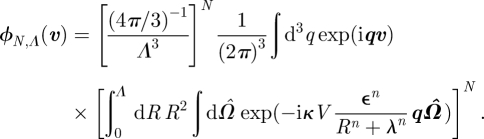
Using spherical variables, X₀^σ = RΩ and for both the initial swimmer positions and velocities, we find

B 3

Introducing a rescaled radial position variable y = R/Λ, and performing the angular integral over , we obtain

B 4a

where

B 4b

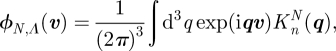
is the characteristic function of ϕ_N,Λ with

B 4c

It is useful to rewrite K_n^N in the equivalent form:

B 5

where K_n(q) is the characteristic function for the one-swimmer case.

B.1.1. Exact second and fourth velocity moments

We note that, for m ∈ N,

B 6a

B 6b

B 6c

B 6d

From these expressions, one finds

B 7a

B 7b

B 7c

B 7d

and, therefore,

B 8a

and

B 8b

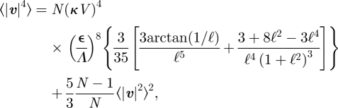
Equations (B 8) hold for any spherically symmetric distribution in three dimensions. From the above expressions, one finds the following exact formulas for the velocity moments in this model:

B 9a

and

B 9b

where,using the abbreviation l := λ/Λ,

B 9c

and

B 9d

For example, for the (n = 2) model, these expressions simplify to

B 10a

and

B 10b

The first integral, and hence 〈|v|²〉_ϕ, diverges as 1/λ if one lets the cut-off λ → 0 (which is equivalent to ℓ → 0). More precisely, in this limit, equations (B 9) reduce in leading order of (Λ/λ) to

B 11a

and

B 11b

where ϕ := N(ε/Λ)³ is the volume filling fraction.

B.1.2. Approximation by a tempered Lévy distribution

We would like to approximate the exact characteristic function K_n^N from equation (B 5) by the tempered Lévy law

B 12

which exhibits quasi-Gaussian behaviour for small q, corresponding to large velocities,

B 13

To motivate the ansatz (B 12), we write equation (B4b) as

B 14

and consider the limit λ = 0. In this case, the double integral for the one-swimmer characteristic function K_n(q) from equation (B 5) can be calculated exactly for n = 1,2,3 in terms of trigonometric, hypergeometric and sine integral functions. By expanding the resulting expressions ln[K_n(q)] for a large volume Λ ≫ ε, one obtains for n = 1 a Gaussian limiting distribution

B 15a

By contrast, for n ≥ 2 the limiting distribution is found to be of the Holtsmark type, i.e.

B 15b

where t_n is a constant of order unity; specifically, and . For comparison, if we let μ→ 0 in equation (B 12), we obtain

B 15c

Thus, by comparing with equations (B 15) and (B 15c), we can identify

B 16a

and

B 16b

Before determining the remaining parameters (c, μ), it is worthwhile to note that the effective temperature scales differently with volume and swimmer number for n = 1 and n ≥ 2, respectively: in the case of a colloidal-type velocity field with n = 1, the effective temperature T₁ is proportional to the area filling fraction N(ε/Λ)², see equation (B 15a), whereas for swimmer-type flow fields with n ≥ 2 the effective temperature T_n scales with the volume filling fraction

B 17

see equation (B 15b). This suggests that, for n = 1, the appropriate thermodynamic limit corresponds to N,Λ→ ∞ while keeping the ratio N/Λ² fixed, whereas for n ≥ 2 one should let N,Λ → ∞ such that N/Λ³ remains constant.

It remains to discuss how to identify the parameters (c,μ), which we shall do next for the cases n = 1,2,3. For n = 1, the procedure is rather straightforward; in the case of n = 2,3, we are going to determine (c,μ) by matching the second and fourth velocity moments of the tempered Lévy ansatz (B 12), which were given in equation (A 11), to the exact moments (B 9).

n = 1. In this case, according to equation (B 16), we have α = 2, and the ansatz (B 12) reduces to the Gaussian

B 18a

By comparing with equation (B 15a), we see that c = T₁, i.e.

B 18b

where we now also included the leading order corrections in ℓ = λ/Λ.

n = 2. In this case, we have α = 3/2 and the velocity moments (A 11) of the tempered Lévy ansatz (B 12) take the form:

B 19a

and

B 19b

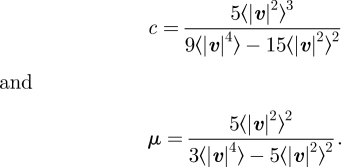
Solving these equations for (c, μ) yields

B 19c

Here, we can insert for 〈|v|²〉 and 〈|v|⁴〉, the exact expressions (B 9); this gives the fit curves shown in figure 2 of the main paper. Furthermore, by expanding the resulting formula for large volume Λ ≫ ε, λ, we find

B 19d

n = 3. In this case, we have α = 1 and the general expression for the velocity moments of the tempered Lévy law from equation (A 11) reduce to

B 20a

and

B 20b

Solving these equations for (c, μ) yields

B 20c

Inserting for 〈|v|²〉 and 〈|v|⁴〉 the exact expressions (B 9) and expanding for Λ ≫ ε, λ, we obtain

B 20d

Note that for a vanishing λ → 0, the parameter μ goes to zero in equations (B 19d) and (B 20d), which implies that the second moment 〈|v|²〉 diverges. This also illustrates why for n ≥ 2—or, more precisely, for n ≥ 3/2 if one allows for non-integer exponents n—there is no convergence to a Gaussian distribution in the limit λ → 0. See figures 2 and 7 in that regard.

Figure 7.

Marginal velocity PDF of a tracer particle in the flow generated by different concentrations of swimmers, using the co-oriented model with (a) n = 1 and (b) n = 2. These one-dimensional PDFs reflect the Gaussian or Lévy nature of their corresponding three-dimensional PDFs. Volume fractions and symbols are those of figure 2.

B.2. Velocity autocorrelation function

We are interested in the fluid's velocity autocorrelation function (A 5b) for the power-law model (B 1). We start from equation (A 5b), which can be written as

B 21

Assuming, as before, that the initial swimmer position and velocities are distributed according to equation (A 3), we can simplify

B 22

Using spherical velocity and position variables, X₀^σ = XΩ and , and inserting the one-swimmer PDF from equation (A 3), we find

B 23

Introducing rescaled variables

B 24a

and noting that

B 24b

we can rewrite equation (B 23) in the form:

B 25

By virtue of the identity

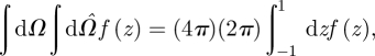B 26

Equation (B 25) can expressed as

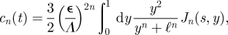B 27a

where

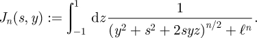B 27b

We next provide explicit results for n = 1 and n = 2.

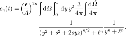
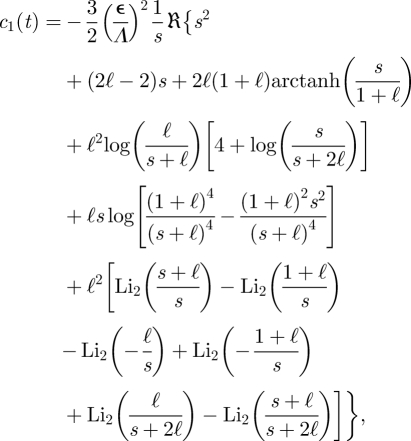
n = 1. In this case, we find

B 28a

The remaining integral y-integration in equation (B 27a) can be easily computed numerically. However, the correlation function c₁(t) can also be expressed analytically in terms of the polylogarithm , defined by

B 28b

and analytical continuation for |z| ≥ 1. is real valued for real z ≤ 1 and possesses the integral representation

B 28c

Considering a sufficiently large volume such that 0 ≤ s ≤ 1, we obtain

B 28d

with ℜ denoting the real part. In particular, in the thermodynamic limit N,Λ → ∞ such that φ = N(ε/Λ)² = const, we find that the autocorrelation function C_N,Λ(t) = N(κV)² c_n (t) becomes constant

B 28e

This situation, however, is unrealistic for real swimmers, which typically generate flow fields that decay with n ≥ 2.

n = 2. In this case, we find

B 29a

Considering again 0 ≤ s ≤ 1, the correlation function c₂(t) may be written in terms of the Dilogarithm Li₂(z) as

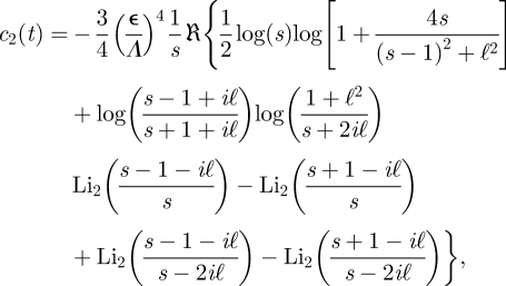B 29b

with ℜ denoting the real part. In the thermodynamic limit N,Λ → ∞ such that φ = N(ε/Λ)³ = const., we find at large times t ≫ τ_ε := ε/V for the full autocorrelation function

B 29c

Appendix C. Second example: Regularized dipolar swimmer model

Let us now consider a more realistic dipolar swimmer flow-field model, defined by

C 1a

where κ > 0 (κ < 0) correspond to an extensile (contractile) swimmer, and

C 1b

As before, we assume, for simplicity, that a swimmer's orientation does not change over time. The dipolar swimmer model (C 1) exhibits the same distance scaling as the regularized power-law model from equation (B 1) with n = 2, but the directional dependence is different. As a consequence, as we shall see below, the velocity PDFs of the two models are very similar but the correlation functions show qualitatively different behaviour.

C.1. Tracer velocity probability density function

C.1.1. Characteristic function

Using spherical variables, X₀^σ = XΩ and for both the initial swimmer positions and velocities, the characteristic function of the velocity PDF can be written as

C 2

where the one-swimmer characteristic function is given by

C 3

Hence, with y := R/λ, ℓ := λ/Λ and ,

C 4

Choosing q = (0,0,|q|) = (0,0,q), with no loss of generality, we find

C 5a

where

C 5b

This result can be used to evaluate analytically the moments of the tracer velocity PDF.

C.1.2. Velocity moments

From equations (C 5) and (B 8), we find the following exact results for the second and fourth velocity moments:

C 6a

and

C 6b

where ℓ := λ/Λ is the rescaled regularization cut-off. In the small cut-off limit ℓ → 0, we find

C 7a

and

C 7b

These expressions are quite similar to those obtained for the power-law model with n = 2, see equation (B 11). The moments (C 7) can be used to determine the parameters of the corresponding tempered Lévy velocity distribution (B 19d) by means of equations (B 12). However, as we shall see below, the two models give rise to very different velocity correlations.

C.2. Velocity autocorrelation function

We are interested in the velocity autocorrelation function (A 5b) of the fluid near the centre of the volume, which can be written as

C 8a

For linear swimmer motions, we further have

C 8b

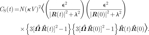
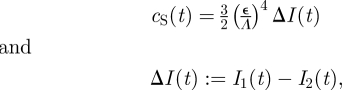
with X and V denoting the initial swimmer position and velocity; Ω and are the corresponding unit vectors. Defining the dimensionless velocity autocorrelation function c_S(t) by C_S = N(κV)²c_S(t), we obtain

C 9

In the limit t = 0, one recovers the second velocity moment, c_S(0) = 〈|v²|〉 /[N(κ V)²].

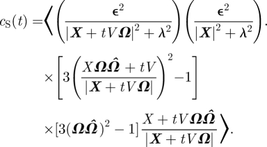
For t > 0, using the notation from equations (B 23) and (B 24), we have

C 10

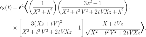
Substituting y := X/Λ, ℓ = λ/Λ, s := tV/Λ and using the identity (B), this can be written as

C 11a

where

C 11b

and

C 11c

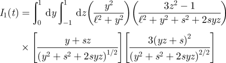
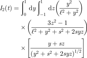
The integration over z can be performed analytically, and the remaining y-integrals can be written as

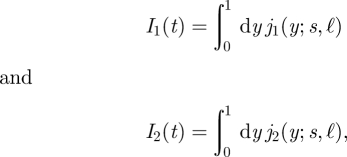C 12a

where

C 12b

and

C 12c

To obtain the exact correlation function, the remaining one-dimensional y-integrals (C 12a) can be computed numerically; for special limit cases, however, one can expand the integrands j_1/2(y;s,ℓ) and evaluate the resulting integrals analytically.

Short-time expansion t → 0

Expanding the integrands j_1/2(y;s,ℓ) at short times s ≪ ℓ, we find

C 13

where ℓ = λ/Λ and s: = tV/Λ.

Large-time (small ℓ) approximation and thermodynamic limit

To obtain an analytically tractable approximation of the autocorrelation function that can be used to determine the thermodynamic limit, we note that, at large times, we can approximate ℓ ≃ 0 in the denominators of the integrals equations (C 11b) and (C 11c). With this simplification, the z-integral can be computed more easily yielding for 0 < s < 1

C 14

where Θ(x) is the unit step function, defined by Θ(x) := 0, x < 0 and Θ(x) := 1,x ≥ 0. In principle, the remaining y integral can readily be evaluated to obtain the long-time behaviour of C_S(t). However, the resulting expression diverges at short times, since we let the cut-off ℓ → 0. To avoid this divergence and mimic the effect of the short-distance cut-off ℓ, we may replace the lower integral boundary in equation (C 14) by a regularization parameter¹ ℓ_*, i.e. we compute

C 15

which gives

C 16a

The regularization parameter ℓ_* can be determined from the condition C_S(0)=〈|v|²〉, by using the exact result (C 6a) for the second moment, yielding

C 16b

The result (C 16) becomes exact at sufficiently large times s → 1; it does, however, also provide a useful approximate description at intermediate and small times. In particular, the second line in equation (C16a) implies that, for a finite system, the autocorrelation function becomes negative after a certain time t₀, which can be estimated as

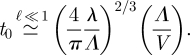C 17

Physically, this is due to the dipolar flow-field structure: if a dipolar swimmer passes a fixed point in the fluid, the flow at this point will reverse its sign (direction) after certain time. However, as evident from equation (C 17), the negative correlation region vanishes for Λ → ∞, as the zero t₀ of c_S(t) moves to ∞ in this limit. More precisely, by taking the thermodynamic limit of equation (C 16), we find that

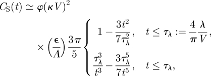C 18

Thus, the velocity field autocorrelation function in a dipolar swimmer suspension decays asymptotically as t⁻³, which is different from the t⁻¹- decay found earlier for the power-law model with n = 2, see equation (B 29c).

C.3. Spatial mean square displacement of a tracer particle

The approximate result for the velocity autocorrelation can be used to obtain an upper bound for the swimmer contribution to the MSD of the tracer particles. Considering an initial tracer position x(0) = 0 and noting that 〈u_N(τ′,0)u_N(τ, 0)〉 = C(|τ′ − τ|), we find

C 19

The second line reflects, roughly speaking, the assumption that correlations are spatially homogeneous and decaying with distance, i.e.

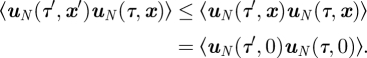C 20

Changing integration variables, τ ↦ θ := τ′ − τ, and, subsequently, τ′ ↦ ν := τ′ − t, we may rewrite equation (C 19) as

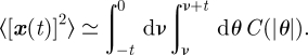C 21

Inserting the approximate result (C 18) for the fluid autocorrelation function in the thermodynamic limit, we find

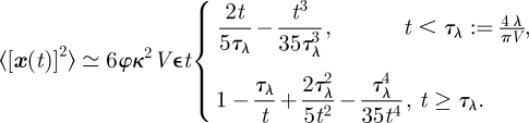C 22

Thus, tracer diffusion in a dilute suspension of dipolar swimmer is ballistic at short times t ≪ τ_λ and normal at large times t ≫ τ_λ.

Appendix D. Numerical methods

In our computer simulations, we directly integrate the Langevin equations

D 1a

D 1b

and

D 1c

where ξ(t) is Gaussian white noise, to obtain the velocity distribution at a given point in the fluid and velocity autocorrelaton functions (for D₀ = 0), and the tracer position PDF (D₀ > 0). The initial positions and velocities Γ^σ(0) = (X₀^σ, V₀^σ) of the swimmers were sampled from the distribution (A 3).

Particle deletion and insertion

Using the Euler method, we simulate an ‘ideal gas’ of active particles (swimmers), which move according to equation (D 1c) through sphere of radius Λ. This sphere is always relative to the passive tracer, whose position evolves according to equation (D 1a). If an active particle leaves the sphere, we immediately delete it. To restore detailed balance, we continually insert new active particles at the boundary of the sphere. The number of insertions per time step is drawn from a Poisson distribution f(j) = ν^j e^−ν/j!, where ν is the mean number of insertions during Δt. We obtain equilibrium by setting ν equal to the mean number of deletions during Δt, which may be estimated from the kinetic theory of gases [42] as ν = (3NV/4Λ)Δt. For each insertion, it is necessary to bias the orientation of an active particle so that its probability distribution satisfies normalized over the solid angle of a hemisphere with inward surface normal . We achieve that by uniformly choosing a position R^σ at a distance Λ relative to the tracer, then choosing an orientation from . Generally, our procedure achieves numerical accuracy if Λ is large, and ensures that a suspension of ballistic particles remains homogeneous and isotropic with mean population N. A comparison with the exact results for time-dependent velocity correlations verifies the validity of this approach.

Graphics processing unit implementation

Resolving the tail of a probability distribution can be a computationally expensive task, even for stochastic processes that are relatively simple. In our numerical calculations, further difficulties arise from having to create and maintain an active suspension unique to each tracer. This process would not be possible in a reasonable amount of time on a traditional computer. We therefore implemented parallelized simulations on a GPU using NVIDIA's Compute Unified Device Architecture (CUDA). Compared with a single-core machine, GPU code yields substantial speed-ups (up to a factor of a few hundreds). However, our longest simulation of 4194304 trajectories still took 14 days on a GPU.

References

- 1.Hänggi P., Marchesoni F. 2005. 100 Years of Brownian Motion. Chaos 15, 026101. 10.1063/1.1895505 (doi:10.1063/1.1895505) [DOI] [PubMed] [Google Scholar]
- 2.IngenHousz J. 1784. Bemerkungen über den Gebrauch des Vergrösserungsglases. In Vermischte Schriften physisch-medicinischen Inhalts, (ed. Molitor N. C.). Wien, Germany: Christian Friderich Wappler [Google Scholar]
- 3.Perrin J. 1909. Mouvement Brownien et réalité moléculaire. Ann. Chim. Phys. 18, 5–114 [Google Scholar]
- 4.Sutherland W. 1905. A dynamical theory of diffusion for non-electrolytes and the molecular mass of albumin. Philos. Mag. 9, 781–785 [Google Scholar]
- 5.Einstein A. 1905. Über die von der molekularkinetischen Theorie der Wärme geforderten Bewegung von in ruhenden Flüssigkeiten suspendierten Teilchen. Annalen der Physik und Chemie 17, 549–560 [Google Scholar]
- 6.Leptos K. C., Guasto J. S., Gollub J. P., Pesci A. I., Goldstein R. E. 2009. Dynamics of enhanced tracer diffusion in suspensions of swimming eukaryotic microorganisms. Phys. Rev. Lett. 103, 198103. 10.1103/PhysRevLett.103.198103 (doi:10.1103/PhysRevLett.103.198103) [DOI] [PubMed] [Google Scholar]
- 7.Purcell E. M. 1977. Life at low Reynolds number. Am. J. Phys. 45, 3–11 10.1119/1.10903 (doi:10.1119/1.10903) [DOI] [Google Scholar]
- 8.Han Y., Alsayed A. M., Nobili M., Zhang J., Lubensky T. C., Yodh A. G. 2006. Brownian motion of an ellipsoid. Science 314, 626–630 10.1126/science.1130146 (doi:10.1126/science.1130146) [DOI] [PubMed] [Google Scholar]
- 9.Li T., Kheifets S., Medellin D., Raizen M. G. 2010. Measurement of the instantaneous velocity of a Brownian particle. Science 328, 1673–1675 10.1126/science.1189403 (doi:10.1126/science.1189403) [DOI] [PubMed] [Google Scholar]
- 10.Drescher K., Goldstein R. E., Tuval I. 2010. Fidelity of adaptive phototaxis. Proc. Natl Acad. Sci. USA 107, 11 171–11 176 10.1073/pnas.1000901107 (doi:10.1073/pnas.1000901107) [DOI] [PMC free article] [PubMed] [Google Scholar]
- 11.Polin M., Tuval I., Drescher K., Gollub J. P., Goldstein R. E. 2009. Chlamydomonas swims with two ‘gears’ in a eukaryotic version of run-and-tumble motion. Science 325, 487–490 10.1126/science.1172667 (doi:10.1126/science.1172667) [DOI] [PubMed] [Google Scholar]
- 12.Leonardo R. D., et al. 2010. Bacterial ratchet motors. Proc. Natl Acad. Sci. USA 107, 9541–9545 10.1073/pnas.0910426107 (doi:10.1073/pnas.0910426107) [DOI] [PMC free article] [PubMed] [Google Scholar]
- 13.Sokolov A., Apodacac M. M., Grzybowskic B. A., Aranson I. S. 2009. Swimming bacteria power microscopic gears. Proc. Natl Acad. Sci. USA 107, 969–974 10.1073/pnas.0913015107 (doi:10.1073/pnas.0913015107) [DOI] [PMC free article] [PubMed] [Google Scholar]
- 14.Chen D. T. N., Lau A. W. C., Hough L. A., Islam M. F., Goulian M., Lubensky T. C., Yodh A. G. 2007. Fluctuations and rheology in active bacterial suspensions. Phys. Rev. Lett. 99, 148302. 10.1103/PhysRevLett.99.148302 (doi:10.1103/PhysRevLett.99.148302) [DOI] [PubMed] [Google Scholar]
- 15.Hernandez-Ortiz J. P., Stoltz C. G., Graham M. D. 2005. Transport and collective dynamics in suspensions of confined swimming particles. Phys. Rev. Lett. 95, 204501. 10.1103/PhysRevLett.95.204501 (doi:10.1103/PhysRevLett.95.204501) [DOI] [PubMed] [Google Scholar]
- 16.Underhill P. T., Hernandez-Ortiz J. P., Graham M. D. 2008. Diffusion and spatial correlations in suspensions of swimming particles. Phys. Rev. Lett. 100, 248101. 10.1103/PhysRevLett.100.248101 (doi:10.1103/PhysRevLett.100.248101) [DOI] [PubMed] [Google Scholar]
- 17.Wu X.-L., Libchaber A. 2000. Particle diffusion in a quasi-two-dimensional bacterial bath. Phys. Rev. Lett. 84, 3017. 10.1103/PhysRevLett.84.3017 (doi:10.1103/PhysRevLett.84.3017) [DOI] [PubMed] [Google Scholar]
- 18.Metzler R., Klafter J. 2000. The random walk's guide to anomalous diffusion: a fractional dynamics approach. Phys. Rep. 339, 1–77 10.1016/S0370-1573(00)00070-3 (doi:10.1016/S0370-1573(00)00070-3) [DOI] [Google Scholar]
- 19.Metzler R., Klafter J. 2004. The restaurant at the end of the random walk: recent developments in fractional dynamics descriptions of anomalous dynamical processes. J. Phys. A. 37, R.61. 10.1088/0305-4470/37/31/R01 (doi:10.1088/0305-4470/37/31/R01) [DOI] [Google Scholar]
- 20.Mantegna R. N., Stanley H. E. 1994. Stochastic process with ultraslow convergence to a Gaussian: the truncated Lévy flight. Phys. Rev. Lett. 73, 2947–2949 10.1103/PhysRevLett.73.2946 (doi:10.1103/PhysRevLett.73.2946) [DOI] [PubMed] [Google Scholar]
- 21.Weeks E. R., Weitz D. A. 2002. Properties of cage rearrangements observed near the colloidal glass transition. Phys. Rev. Lett. 89, 095704. 10.1103/PhysRevLett.89.095704 (doi:10.1103/PhysRevLett.89.095704) [DOI] [PubMed] [Google Scholar]
- 22.Nicodemi M., Coniglio A. 1999. Aging in out-of-equilibrium dynamics of models for granular media. Phys. Rev. Lett. 82, 916–919 10.1103/PhysRevLett.82.916 (doi:10.1103/PhysRevLett.82.916) [DOI] [Google Scholar]
- 23.Drescher K., Goldstein R. E., Michel N., Polin M., Tuval I. 2010. Direct measurement of the flow field around swimming microorganisms. Phys. Rev. Lett. 105, 168101. 10.1103/PhysRevLett.105.168101 (doi:10.1103/PhysRevLett.105.168101) [DOI] [PubMed] [Google Scholar]
- 24.Lauga E., Powers T. R. 2009. The hydrodynamics of swimming microorganisms. Rep. Prog. Phys. 72, 1–36 10.1088/0034-4885/72/9/096601 (doi:10.1088/0034-4885/72/9/096601) [DOI] [Google Scholar]
- 25.Anderson J. L. 1989. Colloid transport by interfacial forces. Ann. Rev. Fluid Mech. 21, 61–99 10.1146/annurev.fl.21.010189.000425 (doi:10.1146/annurev.fl.21.010189.000425) [DOI] [Google Scholar]
- 26.Dunkel J., Putz V. B., Zaid I. M., Yeomans J. M. 2010. Swimmer-tracer scattering at low Reynolds number. Soft Matter 6, 4268–4276 10.1039/c0sm00164c (doi:10.1039/c0sm00164c) [DOI] [Google Scholar]
- 27.Pedley T. J., Kessler J. O. 1990. A new continuum model for suspensions of gyrotactic microorganisms. J. Fluid Mech. 212, 155–182 10.1017/S0022112090001914 (doi:10.1017/S0022112090001914) [DOI] [PubMed] [Google Scholar]
- 28.Baskaran A., Marchetti M. C. 2009. Statistical mechanics and hydrodynamics of bacterial suspensions. Proc. Natl Acad. Sci. USA 106, 15 567–15 572 10.1073/pnas.0906586106 (doi:10.1073/pnas.0906586106) [DOI] [PMC free article] [PubMed] [Google Scholar]
- 29.Simha R. A., Ramaswamy S. 2002. Hydrodynamic fluctuations and instabilities in ordered suspensions of self-propelled particles. Phys. Rev. Lett. 89, 058101. 10.1103/PhysRevLett.89.058101 (doi:10.1103/PhysRevLett.89.058101) [DOI] [PubMed] [Google Scholar]
- 30.Guasto J. S., Johnson K. A., Gollub J. P. 2010. Oscillatory flows induced by microorganisms swimming in two-dimensions. Phys. Rev. Lett. 105, 168101. [DOI] [PubMed] [Google Scholar]
- 31.Gnedenko B. V., Kolmogorov A. N. 1954. Limit distributions for sums of independent random variables. Cambridge, MA: Addison-Wesley [Google Scholar]
- 32.Chandrasekhar S. 1943. Stochastic problems in physics and astronomy. Rev. Mod. Phys. 15, 1–89 10.1103/RevModPhys.15.1 (doi:10.1103/RevModPhys.15.1) [DOI] [Google Scholar]
- 33.Takayasu H. 1984. Stable distribution and Lévy process in fractal turbulence. Prog. Theor. Phys. 72, 471–479 10.1143/PTP.72.471 (doi:10.1143/PTP.72.471) [DOI] [Google Scholar]
- 34.Barkai E., Naumov A. V., Vainer Y. G., Bauer M., Kador L. 2003. Lévy statistics for random single-molecule line shapes in a glass. Phys. Rev. Lett. 91, 075502. 10.1103/PhysRevLett.91.075502 (doi:10.1103/PhysRevLett.91.075502) [DOI] [PubMed] [Google Scholar]
- 35.Barkai E., Silbey R., Zumofen G. 2000, Lévy distribution of single molecule line shape cumulants in glasses. Phys. Rev. Lett. 84, 5339–5342 10.1103/PhysRevLett.84.5339 (doi:10.1103/PhysRevLett.84.5339) [DOI] [PubMed] [Google Scholar]
- 36.Hänggi P., Jung P. 1995. Colored noise in dynamical systems. Adv. Chem. Phys. 89, 239–326 [Google Scholar]
- 37.Samorodnitsky G., Taqqu M. S. 1994. Stable non-gaussian random processes: stochastic models with infinite variance. New York, NY: Chapman & Hall [Google Scholar]
- 38.Shraiman B. I., Siggia E. D. 1994. Lagrangian path-integrals and fluctuations in random flow. Phys. Rev. E 49, 2912–2927 10.1103/PhysRevE.49.2912 (doi:10.1103/PhysRevE.49.2912) [DOI] [PubMed] [Google Scholar]
- 39.Touchette H., Cohen E. G. D. 2009. Anomalous fluctuation properties. Phys. Rev. E 80, 011114. 10.1103/PhysRevE.80.011114 (doi:10.1103/PhysRevE.80.011114) [DOI] [PubMed] [Google Scholar]
- 40.Budini A. A., Cáceres M. 2004. Functional characterization of generalized Langevin equations. J. Phys. A Math. Gen. 37, 5959–5981 10.1088/0305-4470/37/23/002 (doi:10.1088/0305-4470/37/23/002) [DOI] [Google Scholar]
- 41.Rushkin I., Kantsler V., Goldstein R. E. 2010. Fluid velocity fluctuations in a suspension of swimming protists. Phys. Rev. Lett. 105, 188101. [DOI] [PubMed] [Google Scholar]
- 42.Carron N. J. 2007. An introduction to the passage of energetic particles through matter. Boca Raton, FL: CRC Press [Google Scholar]