Estimating reproduction numbers for adults and children from case data

Abstract

We present a method for estimating reproduction numbers for adults and children from daily onset data, using pandemic influenza A(H1N1) data as a case study. We investigate the impact of different underlying transmission assumptions on our estimates, and identify that asymmetric reproduction matrices are often appropriate. Under-reporting of cases can bias estimates of the reproduction numbers if reporting rates are not equal across the two age groups. However, we demonstrate that the estimate of the higher reproduction number is robust to disproportionate data-thinning. Applying the method to 2009 pandemic influenza H1N1 data from Japan, we demonstrate that the reproduction number for children was considerably higher than that of adults, and that our estimates are insensitive to our choice of reproduction matrix.

1. Introduction

When assessing how fast an infectious disease is spreading, there are two key disease characteristics that we need to know: the reproduction number and the serial interval. The effective reproduction number tells us how many people (on average), a randomly selected infected person infects. It differs from the basic reproduction number in that it incorporates the effects of susceptible depletion and any public health interventions, and so is more closely tied to empirically observed data. The mean serial interval is the average delay between one person showing symptoms and the individuals they infect showing symptoms. While the reproduction number may vary by location, over time and according to the level of intervention, we generally expect the serial interval to be consistent between locations and through time, unless rigorous extrinsic measures (such as case isolation and quarantine) influence the contact patterns [1]. In the event of an outbreak of an existing disease, while the distribution of the serial interval may be assumed to be known, dynamic estimates of the reproduction number are urgently needed for the policy makers to assess the local spread of the disease and to determine the probable impact of interventions.

In recent years, a number of methods have been developed for estimating the reproduction number from outbreak data [2–10]. Some of these methods estimate characteristics of the serial interval simultaneously [2,4,9], while others assume that the distribution of the serial interval is known [5–8]. Most methods can only be applied during the early ‘take-off’ phase of an outbreak, and so provide a single estimate of the reproduction number, but some—such as the Wallinga & Teunis method [7] with Cauchemez adjustment [3] (similar to that used in Ferguson et al. [11])—estimate the time-varying reproduction number over the course of the outbreak.

While necessary for assessing overall disease spread, estimates of a single reproduction number for an entire population do not provide information on the underlying heterogeneous transmission within and between different types of individuals. For example, some diseases show an age-specific pattern of infection, with a higher number of cases in a particular age group. Alternatively, some diseases show higher case numbers in a particular ethnic group or other sub-population. Both of these situations occurred during the 2009 pandemic influenza H1N1 outbreak [12,13]. Type structure is routinely included in disease transmission models to allow for dependence on age or other forms of population structure [14,15]. Here, we estimate type-specific reproduction numbers, using adults and children as a case study. This approach provides estimates of the average number of secondary cases that a single individual of each type produces. A comparison of these type-specific reproduction numbers provides us with an understanding of how much adults and children contribute to transmission, which can inform decisions on interventions.

Recent work by Nishiura et al. [16] incorporates age structure into estimates of the reproduction number for a single time period. Here, we present methods for estimating reproduction numbers for two types of individuals over time, allowing us to detect the impact of interventions on different groups, and to monitor changes over the course of an outbreak. While the primary method presented here is an extension of the transmission network method used by Wallinga & Teunis [7], we also compare this with the population growth method used by White & Pagano [9,10]. For simplicity, we will refer to these approaches as the ‘Wallinga & Teunis’ [7] and the ‘White & Pagano’ methods [9,10], although we acknowledge that others have used similar techniques, as outlined above. In this paper, our aim is to quantify the type-specific transmission patterns using daily case numbers stratified by type. We also assess the sensitivity of these estimates to assumptions about transmission between the groups and to under-reporting of case numbers. These methods are applied to 2009 influenza pandemic H1N1 (pH1N1) data from Japan to compare reproduction numbers for adults and children.

2. Methods

2.1. Data

We use both computer-generated simulation data and real pH1N1 incidence counts to test the methods. We do not attempt to estimate the reproduction numbers and characteristics of the serial interval simultaneously, but adopt the distribution of the serial interval estimated from Australian data at the start of the outbreak [17] for both types of individuals. This has a gamma distribution with mean of 2.9 days and s.d. of 1.4 days.

Simulated data are generated from a stochastic transmission model using the various reproduction matrices outlined below. In each simulation, we assume one initial case of type selected according to the proportion in the population. Simulations are assumed to take off if 50 or more cases occur, and are run until there are 2000 cases. In general, 100 simulations are conducted for each scenario. We tested the impact of the type of initial case (i.e either adult or child) on estimates of the type-specific reproduction numbers and found only an early, short-term effect and no effect on the final estimates. The short-term impact of the initial case is no longer visible once there are around 20 cumulative cases (of either type), which is the time at which we begin plotting the time-varying reproduction numbers. To test the effect of under-reporting, we consider outbreaks in which a fraction of either adult cases, child cases or both are not reported. We also apply the method to pH1N1 data from Japan described in the study of Nishiura et al. [16].

2.2. Reproduction matrices

The reproduction matrix for two types of individual has the form

where m_ij denotes the average number of cases of type i infected by a single individual of type j throughout its entire course of infection. In a fully susceptible population, this matrix is often referred to as a next-generation matrix [18].

A key issue is that we can estimate only two parameters for the 2 × 2 matrices, as daily incidence counts give us only two growth rates. If we attempt to estimate all four elements of this matrix from daily case data, we generally find a band of equal-likelihood values pairing matrix elements m_CC with m_CA and m_AC with m_AA (figure 1). In order to estimate two reproduction numbers unambiguously, we must make some assumptions about the form of the reproduction matrix. Here, we consider the influence of the matrix parametrization on the resulting interpretation of the transmission dynamics for the four matrix forms.

Figure 1.

Surface plots showing the likelihood function varying with each of the six pairs of matrix elements m_ij when attempting to fit incidence data generated with proportional matrix [1.75,0.25; 0.75,0.75]. The lighter shades of grey indicate higher values of the likelihood function. The optimum is estimated to be [1.0,0.5; 0.8,0.8]. Fixed elements are taken to be the estimated values.

2.2.1. Symmetric matrices

In analysing the early pH1N1 Japanese data, Nishiura et al. [16] consider two forms for the reproduction matrix: a separable matrix and one with high child-to-child transmission (which we will refer to as HiC2C). The separable reproduction matrix can be separated into row and column parameters, while the HiC2C matrix assumes a high transmission rate between children, with all other parameters equal. This is one of the primary WAIFW matrices adopted by Anderson & May [14] for two age groups. See table 1 for the formulation of these matrices.

Table 1.

Reproduction matrix forms for estimating two reproduction numbers, where p is the proportion of children individuals in the general population, ρ_C is the fraction of a child's contacts that are with children, and ρ_A is the fraction of an adult's contacts that are with adults.

matrix description	matrix form
separable
HiC2C
contact-frequency
proportional

Within the class of symmetric reproduction matrices, these two forms are the ones most suited to estimating reproduction numbers for two types. Other forms of reproduction matrices that are type-specific or which assume that infectivity or susceptibility vary with type are either too restrictive, or cannot be estimated from daily incidence data. See appendix A for further details on this.

2.2.2. Asymmetric matrices

Symmetric matrices are not suitable in all cases. In the case of adults and children, while all children have contact with adults, many adults in the population have little contact with children. That is, we expect the element of the matrix indicating adult–child infection to be smaller than the child–adult element. In the case of the first wave of transmission in Japan [16], the outbreak was centred on a school, so a symmetric pattern of infection is not unreasonable for these initial cases. When the outbreak involves wider community transmission, the assumption of symmetry is less likely to be valid, as many adults involved in the outbreak will not have regular contact with children.

For cases where symmetric reproduction matrices are not appropriate, there are many types of matrix form we could use. Here, we consider two asymmetric matrices: a contact-frequency matrix that uses data on contact patterns to determine mixing between the two groups, and a modified proportional mixing matrix that uses data on the proportion of the population of each type to determine transmission patterns (table 1). It has been recognized that human contact networks tend to be highly assortative—that is, individuals prefer to associate with individuals of the same type [19,20]—and both of these matrix forms allow for assortative mixing.

The contact-frequency matrix is applicable in the case where there are data on the mixing patterns of the two groups. For adults and children, we use data presented in Mossong et al. [20] to calibrate mixing patterns, and assume that 50 per cent of a child's contacts are with other children, while 75 per cent of an adult's contacts are with other adults (that is ρ_C = 0.5 and ρ_A = 0.75). Under this assumption, it should be noted that we do not expect the matrix to satisfy reciprocity [21]; our contact-frequency matrix also includes two parameters to be estimated that allow for differences in infectivity and susceptibility between the two types of individual.

The modified proportional matrix assumes that adults infect other individuals according to their proportions in the population. We assume that children make up 25 per cent of the population, so that 25 per cent of an adult's infections are children and 75 per cent are other adults. We then adjust this proportional matrix to allow for extra transmission between children. For simplicity, we will refer to this matrix form as the proportional reproduction matrix.

Finally, we also consider matrices that do not correspond to any of the above formats to assess the effect of the imposed structure on the estimated reproduction numbers.

2.3. Definition of the type-specific reproduction number

We define the reproduction number for children (adults) as the average number of cases generated by a single infected child (adult) at calendar time t. This quantity is calculated in a different manner in the following two algorithms, but both methods use daily incidence data to fit a transmission matrix of the form M = [m_ij]. The White & Pagano method [9,10] estimates single values for the components of the matrix M, assuming that this matrix remains constant over the initial stages of the outbreak. The Wallinga & Teunis method [7] reconstructs the transmission network in such a way that there is a daily estimate for the reproduction matrix M. For both approaches, the reproduction numbers for the two types of individual are given by the column sums of M, that is:

We use R to refer to the dominant eigenvalue of the matrix M—that is, the population reproduction number. It should be noted that R_C and R_A are different from the so-called type-reproduction number proposed by Roberts & Heesterbeek [22] for computing required public health effort to eradicate an infectious disease. Rather, our R_C and R_A represent the average numbers of secondary cases (inclusive of both child and adult secondary cases) generated by a single child and adult primary case, respectively, and we hereafter refer to these as the ‘type-specific reproduction number’. These type-specific reproduction numbers are useful for assessing ‘I-control’ [23], where interventions act on the infectiousness of the target group, for example, through case isolation and social-distancing measures such as school closure. It is also possible to adapt the methods proposed here to sum row entries of M to assess ‘S-control’, where interventions modify susceptibility of the target group—for instance, using vaccination or antiviral prophylaxis.

2.4. White and Pagano method for estimating type-specific reproduction numbers

Here, we adapt the method used by White & Pagano [9,10] to allow for two types of individual. In this study, we restrict the use of this method to an estimation of the reproduction number during the early ‘take-off’ period of the epidemic. That is, we assume that the transmission matrix is constant over this period, and estimate a single value for each of the two type-specific reproduction numbers. Assume that we have T days of daily incidence data C_t for children and A_t for adults, and the serial interval has a distribution with a probability function w(τ), τ = 1, … , k. In a manner similar to White & Pagano [9,10], we define X_i ∼ Pois(m_CCC_i + m_ACA_i) and Y_i ∼ Pois(m_CAC_i + m_AAA_i) to be the total number of cases of each type infected by individuals with onset on day i. The derivation of the likelihood described in White & Pagano [9,10] can then be reproduced for two types, where we define μ_A and μ_C, the expected number of adult and child cases on day t as

and

The summation over τ includes all cases that may infect a new case on day t, adjusted by the probability of a serial interval of duration τ. The likelihood function then has the form

It is possible to maximize this function with no restrictions on the matrix elements m_ij, however, it is often difficult to distinguish all terms. Figure 1 is an illustrative plot of the likelihood function for each of the six pairs of variables when estimating matrix elements from computer-generated data. There is a band of approximately equal likelihood for the pair m_CC and m_CA and for the pair m_AA and m_AC. This pattern is typical for pH1N1 data as well as computer-generated data.

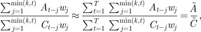
However, if we maximize the likelihood function subject to one of the reproduction matrix forms discussed earlier and given in table 1, the four matrix elements are reduced to two parameters in such a way that the identifiability problem is removed. It is then possible to derive unambiguous estimates for the reproduction matrix entries and the reproduction numbers. Provided the fraction of infected individuals of each type remains approximately constant, we can derive the following two equations in four unknowns that are satisfied by the maximum-likelihood solutions for all matrix forms.

and

where , , and . Note that if the fraction of infected individuals of each type varies over the course of the outbreak, the time-varying reproduction number produced by the Wallinga & Teunis method [7] (which allows for these changes) is more appropriate.

Together with a choice of matrix form, this will allow maximum-likelihood estimates to be calculated algebraically. For instance, with a separable matrix, where m_AC = m_CA and m_AAm_CC = m_ACm_CA, we have:

and

Further details for separable and other matrix forms are given in appendix A.

2.5. Wallinga and Teunis method for estimating type-specific reproduction numbers

Here, we adapt the methods used by Wallinga & Teunis [7] and Cauchemez et al. [3] to allow for two types of individual. These methods for reconstructing the transmission network (or transmission tree) are similar to the estimation framework of the cohort reproduction number in mathematical demography, whose usefulness has recently become apparent in infectious disease epidemiology [24,25]. The Wallinga & Teunis method [7] provides daily estimates of the reproduction number, and thus can be applied to part or all of a disease outbreak. The algorithm estimates the probability that individual i infected individual j on the basis of the gap between the onset days of the two individuals.

Assume that case i has onset time t_i and is of type a_i ∈ {C,A}. Recall that w(τ),τ = 1, …, k is the distribution of the serial interval (common to both adults and children). For a single type of individual, Wallinga & Teunis [7] define

to be the probability that individual i was infected by individual j. They then used this to estimate a reproduction number for individual j as ∑_i≠j p_ij.

We modify these formulae to take account of the type of individuals i and j. Define a weight, q_C, to be the fraction of child cases that are infected by a child (so that 1 − q_C is the fraction of children that are infected by an adult). Similarly, q_A is the fraction of adult cases that are infected by an adult. When assessing the probability that individual j infected individual i, we then compare the gap between onset of i and j with that of other individuals of the same type as j. That is, we have

Note that the denominators of the type-specific estimates sum over individuals, l, of the same type as individual j only. This is done to ensure that the probability that individual i was infected by an individual of the same type is —that is, the probability that a child is infected by a child is q_C in line with the weights defined above. This can be verified algebraically as and . As before, the reproduction number for individual j is given by ∑_i≠j p_ij.

We then calculate daily reproduction numbers for the two types of individuals as

that is, the sum of the estimated number of cases infected by individuals of that type with onset on day t.

It remains to estimate q_C and q_A given the daily incidence counts and a choice of reproduction matrix form. Define f to be the fraction of total cases that are children. Then, for any of the reproduction matrices in table 1, it is possible to express the matrix elements (and thus q_C and q_A) in terms of f and the population reproduction number, R. For instance, for a separable matrix, we can calculate q_C = 1/(1 + x² ) and q_A = x²/(1 + x² ), where x = (1 − f)/f.

During the initial exponential growth phase of an outbreak, we would expect f to be relatively constant, but often f will change over the course of the outbreak. In this case, we use daily values of f to calculate q_C and q_A, and thus allow them to vary with time. Details of q_C and q_A for various matrix forms are given in appendix A.

2.6. Effect of thinning

It is rare that every infected individual is included in surveillance data, particularly if the disease is common or mild. Analysis of methods for estimating the reproduction number for a single type of individual shows that they are robust to under-reporting, even if only a very small proportion of cases are reported [26], provided the proportion of cases reported remains constant over time [27]. When a change in the reporting proportion occurs, this generally impacts the time-dependent estimates of the reproduction number for a time period approximately equal to twice the mean serial interval [28]. For a disease such as influenza, such effects are relatively minor provided they do not occur too frequently. When we consider the impact of thinning on estimates of reproduction numbers for adults and children, we find that they are similarly robust if the proportion of cases reported is equal across the two age groups. However, if the extent of thinning varies between the groups—say because health-workers have been instructed to prioritize the follow-up of at-risk groups—there will be some effect on the estimates of the reproduction numbers.

We investigate the effect of thinning analytically and using simulated datasets with different reproduction matrices assuming that the thinning is constant through time. For a matrix form, we can define the reproduction numbers of the two types in terms of the local population reproduction number (R) and the fraction of cases that are children (f). As discussed above, R is relatively insensitive to thinning, so we focus on assessing the sensitivity of the type-specific reproduction numbers to inaccuracies in f.

3. Results

3.1. Simulation data

We begin by considering estimates of type-specific reproduction numbers from computer-generated data. In figure 2, we present estimates of these reproduction numbers using our modification of the Wallinga & Teunis method [7] from data generated using separable and proportional reproduction matrices for adults and children, assuming children make up 25 per cent of the underlying population. Figure 2a,c,e shows the analysis of the data generated using the separable matrix, and figure 2b,d,f shows the analysis using the proportional matrix. In each case, the matrices used in the simulations have a reproduction number for children (R_C) of 2.5 and a reproduction number for adults (R_A) of 1.0. Estimates of the reproduction number are shown as soon as the cumulative cases (across both groups) reaches 20. Figure 2a,b shows a typical example of simulated data. We see that the fraction of child cases is greater under the separable matrix when compared with the proportional matrix (71% children with the separable matrix versus 60% children with the proportional matrix). As shown by figure 2c,d, the method provides reliable estimates of the reproduction numbers when the same form of reproduction matrix that generated the data are used. Figure 2e,f shows the effect of using a different matrix form. When the data are generated using the separable matrix (figure 2a,c,e), all methods estimate the higher reproduction number reasonably well, but the asymmetric matrix methods (contact-frequency and proportional) underestimate the lower reproduction number. When the data are generated using the proportional matrix (figure 2b,d,f), both symmetric matrices (separable and HiC2C) underestimate the higher reproduction number and overestimate the lower reproduction number.

Figure 2.

Estimates of the reproduction numbers for children and adults (R_C and R_A) from computer-generated data. The data are generated using a separable matrix (a,c,e) and a proportional matrix (b,d,f), each with a reproduction number in the simulation of 2.5 for children and 1.0 for adults. (a,b) The daily incidence counts, (c,d) the estimates for the two reproduction numbers with 95% confidence intervals (using the same matrix form as used to generate the data) and (e,f) the estimates if a different matrix form is assumed. In all cases, children are in black and adults in grey, and estimates of the reproduction numbers begin when there are 20 cumulative cases. In (e,f), the estimates by matrix form are as follows. Solid line, separable; dashed line, HiC2C; dotted-dashed line, contact-frequency; dotted line, proportional.

We also perform these calculations using the modified White & Pagano method [9,10] that gives a single estimate and not a time-varying one. Using the correct matrices, we estimate R_C = 2.47, R_A = 1.02 for the separable matrix, and R_C = 2.63, R_A = 0.91 for the proportional matrix. Again, estimates of R_C are too low and R_A are too high if symmetric matrices are assumed for the proportional data, and estimates of R_A are too low if asymmetric matrices are assumed for separable data.

Table 2 explores this in more detail, giving the 3rd percentile, the median and the 98th percentile of estimates of R_C and R_A for 100 simulations of each type of reproduction matrix, where the values used to generate the data are R_C = 2.5 and R_A = 1.0. By giving lower and upper percentiles, we describe a range that contains 95 per cent of the simulations. We see that all methods perform well if the assumed matrix form matches the original matrix form (the upper diagonal blocks in the table). Assuming a symmetric reproduction matrix, when the original matrix is asymmetric gives poor estimates of both reproduction numbers, with R_C underestimated and R_A overestimated. Estimating an asymmetric reproduction matrix when the original matrix is symmetric leads to an underestimate of R_A, but only a slight overestimate of R_C. Using the wrong asymmetric matrix leads to errors in the estimate of R_A, while both the contact-frequency and proportional reproduction matrices provide good estimates of either type of asymmetric data.

Table 2.

Estimates of R_C and R_A for computer data generated under four different structured reproduction matrices and two unstructured matrices, all with simulated values of R_C = 2.5 and R_A = 1.0. The row indicates the matrix form used to generate the data and the column indicates the assumption made by the estimation method. For each row and column pair, 100 simulations were run and the 3^rd (L), the median (M) and the 98^th (U) estimates are shown for each of R_C and R_A, thus providing a range that contains 95% of the simulations.

assumed true		separable			HiC2C			contact-frequency			proportional
		L	M	U	L	M	U	L	M	U	L	M	U
separable	RC	2.32	2.50	2.65	2.27	2.42	2.58	2.47	2.62	2.79	2.43	2.58	2.77
	RA	0.90	1.00	1.14	1.06	1.20	1.30	0.61	0.70	0.80	0.72	0.80	0.91
HiC2C	RC	2.37	2.57	2.74	2.31	2.49	2.67	2.47	2.64	2.84	2.42	2.60	2.81
	RA	0.67	0.77	0.92	0.87	1.01	1.19	0.47	0.54	0.64	0.59	0.67	0.78
contact	RC	2.04	2.26	2.42	2.00	2.21	2.42	2.28	2.50	2.69	2.29	2.52	2.74
	RA	1.22	1.40	1.54	1.32	1.47	1.65	0.91	1.01	1.14	0.88	0.99	1.11
proportional	RC	1.96	2.20	2.38	2.00	2.15	2.32	2.29	2.46	2.67	2.33	2.50	2.75
	RA	1.29	1.44	1.63	1.37	1.52	1.74	0.93	1.05	1.21	0.92	1.00	1.15
unstructured 1	RC	2.00	2.20	2.37	1.99	2.14	2.33	2.27	2.44	2.63	2.31	2.47	2.64
	RA	1.25	1.41	1.62	1.38	1.50	1.65	0.87	1.03	1.18	0.88	0.99	1.12
unstructured 2	RC	2.41	2.54	2.70	2.37	2.48	2.65	2.44	2.60	2.75	2.40	2.57	2.75
	RA	0.61	0.69	0.79	0.81	0.91	1.06	0.40	0.47	0.54	0.54	0.61	0.72

Finally, the last four rows in the table present estimates for simulations run with two unstructured matrices with R_C = 2.5 and R_A = 1.0. These two unstructured matrices are:

and were chosen to ensure that the force of infection on children is higher than on adults, but such that the matrices do not fit any of the four matrix forms described in this paper. The first matrix was selected to ensure that m_CA > m_AC, with the second (less realistic) matrix satisfying m_AC > m_CA. We see that the methods assuming an asymmetric matrix perform better in estimating parameters from the first matrix, while the methods assuming a symmetric matrix perform slightly better on the second matrix. In both cases, the estimates of R_C from the asymmetric method show little bias, although the estimate of R_A from the second (less realistic) matrix is underestimated. Both of these unstructured matrices assume a higher force of infection on children, leading to higher attack rates in children relative to adults. While there may be scenarios in which the attack rate is greater in adults despite a higher reproduction number in children, we are unlikely to attempt to analyse such data with a method that tests for higher transmission in children.

3.2. Japanese data

Next, we apply these methods to data from the initial stages of the pH1N1 outbreak in Japan [16], which had extremely high case numbers in children. Figure 3 presents the estimates of the reproduction numbers for adults and children using the modified Wallinga & Teunis method [7]. For all matrix forms, the reproduction number for children is considerably higher than that for adults at the start of the epidemic, and remains higher for most of the outbreak. Moreover, although there is slight variability between the estimates of the reproduction numbers for adults with different matrices, the estimates of the reproduction number for children are very similar across all four reproduction matrices. Over the first 8 days of data, the mean estimates of the child reproduction numbers are all close to 2.8, while the reproduction numbers for adults ranges between 0.3 and 0.7.

Figure 3.

Estimates of the reproduction numbers for the Japanese outbreak in school children reported in the study of Nishiura et al. [16]. (a) The estimates of the reproduction number for children R_C in black and the reproduction number for adults R_A in grey using a separable matrix and showing 95% confidence intervals. Estimates begin when there are 20 cumulative cases, with a delay in the adult reproduction number because adult cases did not occur until the 13 May. (b) The graph compares the estimates for the separable (solid lines), HiC2C (dashed lines), contact-frequency (dotted-dashed lines) and proportional (dotted lines) matrices.

Estimating the reproduction matrices for the first 8 days of data (corresponding to 156 cases) using the White & Pagano method [9,10] gives the following matrix estimates:

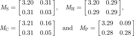for separable (S), HiC2C (H), contact-frequency (C) and proportional (P), respectively. This corresponds to reproduction numbers for children of 3.51, 3.49, 3.52 and 3.57 and reproduction numbers for adults of 0.34, 0.58, 0.21 and 0.37. Again, the results are very consistent across matrix forms for children and show some variation for adults.

Overall, these estimates are a little higher than those of Nishiura et al. [16], but show a similar pattern of high transmission between children. The differences between our estimates and those in Nishiura et al. [16], are largely owing to the difference in the choice of serial interval—Nishiura et al. [16], assume a mean serial interval of 2 days, in contrast to the 2.9 days assumed here. If we adopt a serial interval with mean of 2 days, the estimates of the reproduction numbers for the separable matrix drop to R_C = 2.96, R_A = 0.29 and the HiC2C matrix drop to R_C = 2.93, R_A = 0.47. These are comparable, although slightly lower than the estimates in Nishiura et al. [16]. Throughout this work, we have assumed that the distribution of the serial interval remains constant throughout the epidemic, and is the same for adults and children. Should data be available to identify changes in the serial interval over time [29] or differences between adults and children, this could be incorporated into the estimates of the reproduction numbers.

3.3. Thinned data

In figure 4, we show the results of testing the effect of data thinning on the estimates of the reproduction numbers for two types of individual using computer-generated data with reproduction numbers R_C = 2.5 and R_A = 1. We perform 100 simulations for each of the four matrix forms, taking the final estimate of the reproduction numbers calculated by the method. The results are broadly consistent across matrix forms. If the data are thinned evenly across the two types, both estimates are unbiased. If the child data are thinned, the reproduction number for adults is overestimated and the reproduction number for children is slightly underestimated for some matrices. If the adult data are thinned, the reproduction number for adults is underestimated and the reproduction number for children is slightly underestimated.

Figure 4.

Effect of thinned data on two-type estimates. The figure presents a summary of 100 simulations with R_C = 2.5 and R_A = 1.0 (shown by the dotted lines) for the four matrix forms considered in this paper. The symbol indicates the median estimate of the 100 simulations for the last calculated values of the reproduction numbers. The interval shows the range from the 34rd to the 98th percentile, such that it contains 95% of the simulations. In each case, we compare no thinning, removing 50% of both types, removing 50% of child cases and removing 50% of adult cases. Circles, no thinning; squares, both thinned; diamonds, child thinned; inverted triangles, adult thinned.

We are also interested to see how these results compare for different underlying values of R_C and R_A. We consider only the case where children are disproportionately represented in the data—that is, where R_C > R_A, and the data are not disproportionately thinned to the extent that the proportion of child cases in the dataset is less than the proportion of children in the population. In figure 5, we repeat the analysis of figure 4 for the case where R_C = 2.5 and R_A = 1.5, where the data are thinned to 70 per cent of their original value. The results are similar to those in figure 4, although the estimate of R_C is more biased in the case where the child data are thinned, while the estimate of R_C is generally less biased when the adult data are thinned.

Figure 5.

Summary of 100 simulations with R_C = 2.5 and R_A = 1.5 (shown by the dotted lines) for the four matrix forms. The symbol indicates the median estimate of the 100 simulations for the last calculated values of the reproduction numbers. The interval shows the range from the 3rd to the 98th percentile such that it contains 95% of the simulations. In each case, we compare no thinning, removing 30% of both types, removing 30% of child cases and removing 30% of adult cases. Circles, no thinning; squares, both thinned; diamonds, child thinned; inverted triangles, adult thinned.

Analysis of the various matrix forms in appendix A confirms the results displayed above. Provided child cases are disproportionately represented, estimates of their reproduction number are robust to thinning, generally lying at most 20–30% away from the original value. In the case of the symmetric matrices, the condition that children be disproportionately represented means that over 50 per cent of cases must be in the high-transmission group. In the case of the proportional matrix, we require the fraction of cases to be greater than p (i.e. at least 25% of cases in children in our example). In the case of the contact-frequency matrix, we require (f(1 − ρ_C ))/(1 − f)(1 − ρ_A )> 1, which translates to at least 33 per cent of cases in children for our example. If these conditions hold, the larger reproduction number is closely tied to the population reproduction number (R), and is relatively insensitive to thinning. In contrast, the estimate of the lower reproduction number (adults in this case) is biased.

4. Discussion

These results demonstrate that it is possible to estimate reproduction numbers for adults and children given only daily incidence counts for each group, provided some reasonable assumptions are made about the form of the reproduction matrix. Such estimates provide epidemiological insights into the age-specific transmission over the course of the epidemic, which can allow for more effective targeting of control measures. The methods presented here allow for realistic forms for the distribution of the serial interval, and the Wallinga & Teunis method [7] monitors changes in the reproduction numbers over time.

There are, however, some circumstances under which these methods fail to identify differences between adults and children. For instance, if mixing patterns are such that the disease reproduction number is higher in infected children than infected adults, but the force of infection is higher on adults than on children, these methods will not detect a difference in the reproduction numbers. Additionally, if child case data are thinned much more extensively than adult data such that the resulting proportion of child cases in the dataset is roughly equal to the proportion of children in the population, we will not detect a difference between the reproduction numbers. In contrast, we have demonstrated that evidence of a higher reproduction number in children is robust to mixing and thinning assumptions. Moreover, by outlining four different mixing assumptions, we provide scope to compare the output under different reproduction matrices to assess the extent to which these assumptions may have influenced the results. This helps to identify the level of uncertainty with respect to contact patterns that exist for a particular dataset—as highlighted in Farrington et al. [30], mixing assumptions can have a profound impact on estimates of the reproduction number.

In many studies of infectious disease transmission, reproduction matrices are assumed to be symmetric. That is, they assume that if a randomly selected child infects n adults on average, then a randomly selected adult will infect n children on average. This is often not appropriate for mixing between adults and children, as many adults have very little contact with children. Adopting a symmetric reproduction matrix for data split into adults and children will only identify higher transmission from children if child cases outnumber adult cases. If children do not outnumber adults in the dataset, but are nonetheless disproportionately represented, an asymmetric matrix is generally more appropriate.

In this paper, we consider two asymmetric matrices in detail: a proportional matrix and a contact-frequency matrix. The proportional reproduction matrix allows for extra transmission between one group, with the remaining transmission determined by the proportion of each type of individual in the population. This is a relatively flexible matrix form, as data on the proportion of the population that is in a particular age or ethnic group are generally easy to obtain. The contact-frequency reproduction matrix uses data on the contact patterns of the two types of individuals to determine mixing patterns, and then uses data to estimate differences in the susceptibility or infectivity between the two types of individual. While in many cases this is a more realistic matrix form, it also relies on data that are often not available. We have calibrated our model using European data [20], however, we note that even within Europe there is some variability between countries. The true patterns for Japan—or any other country—may well differ from our assumptions. However, it is reassuring to observe that the estimates of the reproduction numbers derived from the proportional and the contact-frequency matrices are very similar, both for simulated and real data. In future work, we hope to explore further the possible matrix forms to identify more generally the type of information that can be estimated under different matrix assumptions.

When incidence data are collected for a widespread outbreak, we anticipate that they will be considerably thinned. That is, only a proportion of the total cases will be recorded in the dataset. When the reproduction number is estimated for the population as a whole using the Wallinga & Teunis method [7], the estimate is remarkably robust to thinning—provided the proportion of individuals recorded in the dataset does not change markedly over time [26]. If thinning is consistent across types, the same is true of the two-type estimates. If thinning differs between types, there can be biases in the estimates of the reproduction numbers, but this is most apparent for the type with lower reproduction number (adults in the examples considered here). Provided the type with the higher reproduction number (children) are disproportionately represented in the data, estimates of this reproduction number have much less bias. Our simulations and analysis show that this arises because the reproduction number of the type with high transmission is tightly linked to the underlying population reproduction number, which itself is robust to data thinning. This higher reproduction number is critical for informing control measures as it identifies the groups with highest spread of infection. While detailed studies of transmission with recording of all cases remains the gold standard for estimating epidemiological parameters, such studies are rarely undertaken during outbreak situations. The methods presented here allow us to use data that are readily collected to test for differences in disease spread between two types of individuals, and give us an estimate of the reproduction number for the high-transmission group that is relatively free of bias.

Appendix A

We give further details of calculations for the four reproduction matrix forms used in the main text, and outline alternative matrix forms that are less informative. For simplicity of notation, we assume throughout that the two types of individual are adults (A) and children (C), and refer to the corresponding reproduction numbers as R_A and R_C.

For the White & Pagano method [9,10], define the daily case numbers to be A_t and C_t, and set , , .

In order to calculate unambiguous estimates of the reproduction numbers, we assume

that is, that the proportion of infected individuals in each class is approximately constant over time. Under these conditions, the following equations hold

If the proportion of individuals in each class does change over the course of the outbreak, then it is likely that the reproduction numbers also change over time, and the Wallinga & Teunis method [7] should be used instead.

For the Wallinga & Teunis method [7], we define f = C/(A + C) to be the fraction of cases that are children, either for the entire outbreak or daily as f(t). When assessing data thinning, we assume that the population reproduction number, R, is relatively insensitive to thinning [26], and assess the sensitivity of the two reproduction numbers to errors in the estimate of f. In the case of the symmetric matrices (separable and HiC2C), we assume f ≥ 0.5, in the case of the proportional matrix, we assume f ≥ p and in the case of the contact-frequency matrix, we assume ((1 − ρ_C)f)/(1 − ρ_A)(1− f)> 1 to ensure that R_C ≥ R_A.

A.1. Separable matrix

The reproduction matrix has the form .

White & Pagano

We have

and

Wallinga & Teunis

The dominant eigenvalue of this matrix is R = a² + b², and we set x = (1 − f)/f. By definition, q_C = a²f/(a²f + ab(1 − f)) = a²f/Rf = a²/R, and similarly q_A = b²/R. Further, a²f + ab(1 − f) = fR and abf + b² (1 − f) = (1 − f)R, which simplifies to a² + abx = R and ab + b²x = xR. Some algebra then gives us q_C = 1/(1 + x²), q_A = x²/(1 + x² ), R_C = (R(1 + x))/(1 + x²) and R_A = (Rx(1 + x))/(1 + x²) and the reproduction matrix has form

Sensitivity to thinning

R_C is maximized at , and we assume f ≥ 0.5, which implies that R_C ∈ R[1,1.21], since R_C(f = 1/2) = R_C(f = 1) = R and . In contrast, R_A ∈ R[0,1].

A.2. HiC2C matrix

The reproduction matrix has the form

White & Pagano

We have

and the reproduction numbers are

Wallinga and Teunis

We have q_C = 1 − (1 − f)²/f and q_A = 1 − f. The mean reproduction numbers are:

Sensitivity to thinning

As above, R_C is maximized at . We assume f ≥ 0.5, which implies that R_C ∈ R[1,1.17], since R_C(f = 1/2) = R_C(f = 1) = R and . Again, R_A ∈ R[0,1].

A.3. Contact frequency

The reproduction matrix has the form

where ρ_C is the fraction of a child's contacts that are with children, and ρ_A is the fraction of an adult's contacts that are with adults.

White & Pagano

We have

where a is the solution of

Wallinga & Teunis

We have

where q_C is the solution between 0 and 1 of

Sensitivity to thinning

Analysing the effect of thinning on the reproduction numbers is more complicated for the contact-frequency case as there are two parameters in the model. However, if we fix them at ρ_A = 0.75 and ρ_C = 0.5 (as throughout this paper), we find that R_C ∈ R[1,1.29] and R_A ∈ R[0,1].

A.4. Proportional

The reproduction matrix has the form

where p is the fraction of children in the population, assumed to be known.

White & Pagano

We have

and

and

Wallinga & Teunis

We have q_C = (f − p + fp − f²p)/f(1 − p), q_A = 1 − f. The reproduction numbers are R_C = (R(2f − p − f²))/f(1 − p), R_A = (R(1 − f))/(1 − p) and the matrix has the form

Sensitivity to thinning

Assuming f ≥ p, R_C ∈ R[1,K], where . For p = 0.25, K ≈ 1.333. We also have R_C(f = p) = R_C(f = 1) = R. Once again, R_A ∈ R[0,1].

A.5. Type-specific transmission

If the matrix has the form

then all individuals have the same reproduction number, which is not informative. A matrix of the form

also places considerable restrictions on the pairs of reproduction numbers that can be estimated—for instance, this form cannot distinguish between the reproduction numbers for adults and children in the Japanese dataset shown in figure 3.

A.6. Lower diagonal matrix

An alternative asymmetric matrix can be constructed by assuming that there is no transmission from adults to children, giving a matrix of the form

This format gives results similar to the two asymmetric matrices outlined above, but is less flexible.

A.7. Varying infectivity or susceptibility

If infectivity varies with type, the matrix has the form

Then, we have f = 0.5 for all values of a and b. Although the reproduction numbers are different (children have reproduction number 2a, and adults, 2b), we cannot observe these differences from the data.

If susceptibility varies with type, the matrix has the form

and all individuals have reproduction number (a + b).

References

- 1.Lipsitch M., Bergstrom C. T. 2004. Invited commentary: real-time tracking of control measures for emerging diseases. Am. J. Epidemiol. 160, 517–519 10.1093/aje/kwh256 (doi:10.1093/aje/kwh256) [DOI] [PubMed] [Google Scholar]
- 2.Becker N. G., Wang D., Clements M. 2010. Type and quantity of data needed for an early estimate of transmissibility when an infectious disease emerges. Euro Surveill. 15, 19603. [PubMed] [Google Scholar]
- 3.Cauchemez S., Boélle P.-Y., Thomas G., Valleron A.-J. 2006. Estimating in real time the efficacy of measures to control emerging communicable diseases. Am. J. Epidemiol. 164, 591–597 10.1093/aje/kwj274 (doi:10.1093/aje/kwj274) [DOI] [PubMed] [Google Scholar]
- 4.Chowell G., Nishiura H., Bettencourt L. M. A. 2007. Comparative estimation of the reproduction number for pandemic influenza from daily case notification data. J. R. Soc. Interface 4, 155–166 10.1098/rsif.2006.0161 (doi:10.1098/rsif.2006.0161) [DOI] [PMC free article] [PubMed] [Google Scholar]
- 5.Cintrón-Arias A., Castillo-Chávez C., Bettencourt L. M. A., Lloyd A. L., Banks H. T. 2009. The estimation of the effective reproductive number from disease outbreak data. Math. Biosci. Eng. 6, 261–282 [DOI] [PubMed] [Google Scholar]
- 6.Nishiura H., Chowell G., Safan M., Castillo-Chavez C. 2010. Pros and cons of estimating the reproduction number from early epidemic growth rate of influenza A (H1N1) 2009. Theor. Biol. Med. Model. 7, 1–9 10.1186/1742-4682-7-1 (doi:10.1186/1742-4682-7-1) [DOI] [PMC free article] [PubMed] [Google Scholar]
- 7.Wallinga J., Teunis P. 2004. Different epidemic curves for severe acute respiratory syndrome reveal similar impacts of control measures. Am. J. Epidemiol. 160, 509–516 10.1093/aje/kwh255 (doi:10.1093/aje/kwh255) [DOI] [PMC free article] [PubMed] [Google Scholar]
- 8.Wearing H. J., Rohani P., Keeling M. J. 2005. Appropriate models for the management of infectious diseases. PLoS Med. 2, 621–627 10.1371/journal.pmed.0020174 (doi:10.1371/journal.pmed.0020174) [DOI] [PMC free article] [PubMed] [Google Scholar]
- 9.White L. F., Pagano M. 2008. A likelihood-based method for real-time estimation of the serial interval and reproductive number of an epidemic. Stat. Med. 27, 2999–3016 10.1002/sim.3136 (doi:10.1002/sim.3136) [DOI] [PMC free article] [PubMed] [Google Scholar]
- 10.White L. F., Pagano M. 2008. Transmissibility of the influenza virus in the 1918 pandemic. PLoS ONE 3, e1498. 10.1371/journal.pone.0001498 (doi:10.1371/journal.pone.0001498) [DOI] [PMC free article] [PubMed] [Google Scholar]
- 11.Ferguson N. M., Donnelly C. A., Anderson R. M. 2001. Transmission intensity and impact of control policies on the foot and mouth epidemic in great britain. Nature 413, 542–548 10.1038/35097116 (doi:10.1038/35097116) [DOI] [PubMed] [Google Scholar]
- 12.Miller E., Hoschler K., Hardelid P., Stanford E., Andrews N., Zambon M. 2010. Incidence of 2009 pandemic influenza A H1N1 infection in England: a cross-sectional serological study. Lancet 375, 1100–1108 10.1016/S0140-6736(09)62126-7 (doi:10.1016/S0140-6736(09)62126-7) [DOI] [PubMed] [Google Scholar]
- 13.Paine S., et al. 2010. Transmissibility of pandemic influenza A(H1N1)v during the 2009 influenza season in New Zealand: determining the effective reproduction number and the influence of age, ethnicity and importations. Euro Surveill. 15, 19591. [PubMed] [Google Scholar]
- 14.Anderson R. M., May R. M. 1991. Infectious diseases of humans. Dynamics and control. Oxford, UK: Oxford University Press [Google Scholar]
- 15.Diekmann O., Heesterbeek J. A., Metz J. A. 1990. On the definition and the computation of the basic reproduction number R0 in models for infectious diseases in hetergeneous populations. J. Math. Biol. 28, 365–382 10.1007/BF00178324 (doi:10.1007/BF00178324) [DOI] [PubMed] [Google Scholar]
- 16.Nishiura H., Castillo-Chavez C., Safan M., Chowell G. 2009. Transmission potential of the new influenza A(H1N1) virus and its age-specificity in Japan. Euro Surveill. 14, 19227. [DOI] [PubMed] [Google Scholar]
- 17.McBryde E. S., Bergeri I., van Gemert C., Rotty J., Headley E. J., Simpson K., Lester R. A. 2009. Early transmission characteristics of influenza A(H1N1)v in Australia: Victorian state, 16 May–3 June 2009. Euro Surveill. 14, 19363. [DOI] [PubMed] [Google Scholar]
- 18.Diekmann O., Heesterbeek J. A. P., Roberts M. G. 2010. The construction of next-generation matrices for compartmental epidemic models. J. R. Soc. Interface 7, 873–885 10.1098/rsif.2009.0386 (doi:10.1098/rsif.2009.0386) [DOI] [PMC free article] [PubMed] [Google Scholar]
- 19.Newman M. E. J. 2002. Assortative mixing in networks. Phys. Rev. Lett. 89, 208701. 10.1103/PhysRevLett.89.208701 (doi:10.1103/PhysRevLett.89.208701) [DOI] [PubMed] [Google Scholar]
- 20.Mossong J., et al. 2008. Social contacts and mixing patterns relevant to the spread of infectious diseases. PLoS Med. 5, e74. 10.1371/journal.pmed.0050074 (doi:10.1371/journal.pmed.0050074) [DOI] [PMC free article] [PubMed] [Google Scholar]
- 21.Wallinga J., Teunis P., Kretzschmar M. 2006. Using data on social contacts to estimate age-specific transmission parameters for respiratory-spread infectious agents. Am. J. Epidemiol. 164, 936–944 10.1093/aje/kwj317 (doi:10.1093/aje/kwj317) [DOI] [PubMed] [Google Scholar]
- 22.Roberts M. G., Heesterbeek J. A. P. 2003. A new method for estimating the effort required to control an infectious disease. Proc. R. Soc. Lond. B 270, 1359–1364 10.1098/rspb.2003.2339 (doi:10.1098/rspb.2003.2339) [DOI] [PMC free article] [PubMed] [Google Scholar]
- 23.Heesterbeek J. A. P., Roberts M. G. 2007. The type-reproduction number T in models for infectious disease control. Math. Biosci. 206, 3–10 10.1016/j.mbs.2004.10.013 (doi:10.1016/j.mbs.2004.10.013) [DOI] [PubMed] [Google Scholar]
- 24.Fraser C. 2007. Estimating individual and household reproduction numbers in an emerging epidemic. PLoS ONE 2, e758. 10.1371/journal.pone.0000758 (doi:10.1371/journal.pone.0000758) [DOI] [PMC free article] [PubMed] [Google Scholar]
- 25.Nishiura H., Chowell G. 2009. The effective reproduction number as a prelude to statistical estimation of time-dependent epidemic trends. In Mathematical and statistical estimation approaches in epidemiology. New York, NY: Springer; 10.1007/978-90-481-2313-1_5 (doi:10.1007/978-90-481-2313-1_5) [DOI] [Google Scholar]
- 26.Caley P., Philp D. J., McCracken K. 2008. Quantifying social distancing arising from pandemic influenza. J. R. Soc. Interface 5, 631–639 10.1098/rsif.2007.1197 (doi:10.1098/rsif.2007.1197) [DOI] [PMC free article] [PubMed] [Google Scholar]
- 27.White L. F., Pagano M. 2010. Reporting errors in infectious disease outbreaks, with an application to pandemic influenza A/H1N1. Epidemiol. Perspect. Innov. 7, 12. [DOI] [PMC free article] [PubMed] [Google Scholar]
- 28.Mercer G. N., Glass K., Becker N. G. In press Effective reproduction numbers are commonly overestimated early in a disease outbreak. Stat. Med. [DOI] [PubMed] [Google Scholar]
- 29.Kenah E., Lipsitch M., Robins J. M. 2008. Generation interval contraction and epidemic data analysis. Math. Biosci. 213, 71–79 10.1016/j.mbs.2008.02.007 (doi:10.1016/j.mbs.2008.02.007) [DOI] [PMC free article] [PubMed] [Google Scholar]
- 30.Farrington C. P., Kanaan N. M., Gay N. J. 2001. Estimation of the basic reproduction number for infectious diseases from age-stratified serological survey data. Appl. Stat. 50, 251–292 10.1111/1467-9876.00233 (doi:10.1111/1467-9876.00233) [DOI] [Google Scholar]