Anatomy of a chaotic attractor: Subtle model-predicted patterns revealed in population data

Abstract

Mathematically, chaotic dynamics are not devoid of order but display episodes of near-cyclic temporal patterns. This is illustrated, in interesting ways, in the case of chaotic biological populations. Despite the individual nature of organisms and the noisy nature of biological time series, subtle temporal patterns have been detected. By using data drawn from chaotic insect populations, we show quantitatively that chaos manifests itself as a tapestry of identifiable and predictable patterns woven together by stochasticity. We show too that the mixture of patterns an experimentalist can expect to see depends on the scale of the system under study.

The concept of chaos, i.e., that simple deterministic rules can produce complex fluctuations that look stochastic, has fascinated scientists for decades. The suggestion of May (1), that simple deterministic rules might explain the complex fluctuations observed in animal abundances, led to an intense search for chaos in extant population data (2–11). The results have been suggestive but equivocal (7, 12–19), and May's hypothesis remains the subject of lively debate (20–22). Taking a different approach, Costantino and coworkers (23–25) induced chaos in laboratory insect populations. These chaotic cultures were maintained for >8 years (≈70 generations). The resulting long time series afford a unique opportunity to study how chaos is actually expressed in population data (21, 26) and, more generally, to develop better methods of teasing out the deterministic components of natural population fluctuations.

In a pair of pioneering contributions, Schaffer and coworkers (27, 28) drew attention to the fact that chaotic dynamics display episodes of predictable cyclic patterns and that this feature distinguishes them from purely stochastic dynamics. Nevertheless, the perception persists that the inclusion of stochasticity in chaotic models invariably “washes out” such fine detail (see chapter 3 in ref. 29). In this work, we show to the contrary that stochasticity in fact may help to reveal underlying deterministic patterns and, in particular, that subtle temporal patterns associated with deterministic chaos can indeed make themselves manifest. Our study of these data illustrates that, when influenced by deterministic chaos, biological population fluctuations can be expected to display a tapestry of identifiable and predictable near-cyclic patterns woven together by stochasticity.

The experiments that documented chaos in laboratory populations were guided by a discrete-time, continuous-state, stage-structured population model, the so-called larva, pupa, adult (LPA) model (Eq. 1). Manipulation of a demographic parameter induced a sequence of model-predicted dynamic transitions (bifurcations) including a transition to chaos. These studies revealed that, in biological population data, the signal of deterministic chaos is modulated in two important ways. First, the discreteness of individual organisms creates recurrent patterns (termed lattice effects), the structure of which depends on the granularity of system states (30, 31). Second, because births and deaths do not conform to a rigid schedule, variability in the timing of these events, otherwise known as demographic stochasticity, is present in even the most carefully controlled experiments (24). To take account of the discreteness of individuals, we formulated the deterministic discrete-state (or lattice) LPA model (Eq. 2). To account for demographic stochasticity, we formulated a stochastic discrete-state LPA model (Eq. 3).

Deterministically chaotic systems vary over a continuum of system states and display intricate transient temporal structures. These structures are associated with cycles of saddle stability-type, which cause near-cyclic patterns to recur in time series (27, 28, 30, 32–39). When system states are discretized, as in Eq. 2, the chaotic attractor, in general, is broken into multiple cycles with patchy basins of attraction. Fluctuations are cyclic, with periods dependent on initial conditions (40, 41). If stochasticity is introduced into such a system, as in Eq. 3, the system episodically visits each of the cycles, weaving them together in such a way as to recover the signal of the chaotic dynamics. This is the analogue of chaos in a noisy discrete-state system.

Models and Predicted Cycles

The continuous-state deterministic LPA model is

[1]

Here L_t, P_t, and A_t are the number of feeding larvae at time t, the number of nonfeeding larvae, pupae, and callow adults at time t, and the number of sexually mature adults at time t, respectively. The unit of time is 2 weeks, the approximate amount of time spent in each of the L and P classes under our experimental conditions. b > 0 is the average number of larvae recruited per adult per unit time in the absence of cannibalism, and the fractions μ_a and μ_l are the adult and larval probabilities, respectively, of dying from causes other than cannibalism in one time unit. The exponentials represent the fractions of individuals surviving cannibalism one unit of time, with “cannibalism coefficients” c_ea/V, c_el/V, and c_pa/V > 0. Habitat size V has units equal to the volume occupied by 20 g of flour, the amount of medium routinely used in our laboratory.

In the experiment to document chaos (see Appendix), the parameters μ_a and c_pa were manipulated by means of the necessarily integerized equation

where “round” denotes the operation of rounding to the nearest integer (0.5 rounded up). Thus, one possible deterministic discrete-state model for the experiment in question, and the one we used, is

[2]

The stochastic discrete-state model used here is

[3]

where E_1t and E_2t are normal random variables with mean zero and variance–covariance matrix Σ. Parameter values are given in Appendix. In simulations, when a large negative E_it causes a negative value inside a square, we set the right-hand side of that equation equal to zero.

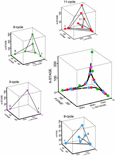
In the continuous-state LPA model (Eq. 1), the dynamics are chaotic and strongly influenced by a saddle-cycle of period 11 (35) (Fig. 1). In the discrete-state LPA model (Eq. 2), all trajectories are eventually periodic, and in fact each trajectory quickly settles onto one of precisely nine periodic orbits. However, these nine orbits fall into three groups of different periodicity: 3-cycles, 6-cycles, and 8-cycles. Furthermore, the orbits within each group lie near one another on the lattice, differing from one another by <30 animals. To clarify the presentation, we chose one representative cycle from each group (Fig. 1). We set out to determine whether these model-predicted temporal patterns were distinguishable in experimental data.

Fig. 1.

Model-predicted continuum and lattice cycles. In the central graph, all cycles that play a role in the present article are superimposed on the chaotic attractor of the deterministic model (Eq. 1). The surrounding graphs depict the four cycles individually. The 11-cycle is from the continuous-state model (Eq. 1); the 8-, 6-, and 3-cycles are from the discrete-state deterministic model (Eq. 2). The phase-space graphs were generated by using conditional least-squares parameter estimates (24).

Pattern Identification

Because the continuous- and discrete-state deterministic models are intimately related, it is not surprising to find that the patterns predicted by the two models have much in common (see Fig. 1). To identify model-predicted cycles in either experimental or simulated data, we used a method we call the lag-metric comparison (LMC). Heuristically, the LMC quantifies the distance (in three-dimensional state space) from a data orbit to a model-predicted periodic orbit of period T, or T-cycle. A precise definition of the LMC is given in Appendix.

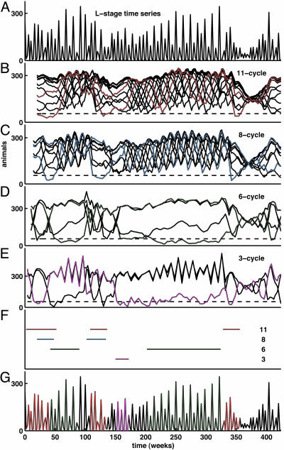
Pattern identification is aided by means of a plot of LMC vs. time as a braid with one strand for each phase. A low LMC value is an indication that the data lie close to the model-predicted cycle and have done so over the course of the preceding T time units. On the other hand, a high LMC value indicates poor correspondence between the data and the model cycle. For example, in Fig. 2B the data are compared with the model 11-cycle. The LMC for each phase of the 11-cycle is given over the 424-week length of the data. The LMC values range from 0 (which indicates an exact match between the model-predicted 11-cycle and an observed length-11 segment of the data) to 300 (which indicates that the observed length-11 segment is an average of 300 animals from the model-predicted 11-cycle).

Fig. 2.

Lag metrics in the data. The LMC is defined in Appendix. (A) Raw time-series data. For clarity, only the L-stage numbers are shown. (B–F) LMC with respect to the model-predicted cycles: continuous-state model saddle 11-cycle (B); discrete-state model 8-cycle (C); discrete-state model 6-cycle (D); and discrete-state model 3-cycle (E). During intervals for which the “braid” appears tightly plaited, the data bear little or no resemblance to the corresponding model-predicted cycle. Unplaited portions of the braid correspond to intervals for which the data closely resemble the model cycle. As shown in F, we identified T-cycle episodes by setting the threshold number of animals θ = 55 (dashed line) and threshold duration K = 12 (see Appendix) for all model-predicted cycles. Thus, to be identified as a T-cycle episode in F, non-equilibrium patterns were required to be in evidence for 24 consecutive weeks (more than seven generations), a very stringent requirement. The effects of varying θ and/or K on the episodes identified can be readily seen from inspection of the LMC plots in B–E.(G) L-stage time-series data as in A, with 11-, 6-, and 3-cycle episodes identified by red, green, and magenta, respectively, corresponding to Figs. 1 and 3.

In the LMC plot, time intervals over the course of which the data resemble the model-predicted cycle (“cycle episodes,” for short) are clearly indicated by corresponding unplaited portions of the braid. Over these intervals, one strand, corresponding to a particular phase of the T-cycle, remains low. Intervals during which the data do not resemble the model-predicted cycle appear tightly plaited. This plaiting and unplaiting of the LMC strands is the characteristic feature of the dynamics we observe, both in simulations of Eqs. 1 and 3 and in experimental data. To illustrate, consider the LMC for the 11-cycle as given in Fig. 2B. At the outset of the experiment, the strands are collectively unplaited. However, around week 50, the strands of the LMC start to entwine, indicating that the time series of data have diverged from the model 11-cycle.

The complete 424-week L-stage data time series is shown in Fig. 2 A (but keep in mind that all life stages are used in computing the LMC). The LMCs for the experimental data with respect to each of the continuous-state and discrete-state model-predicted cycles are shown in Fig. 2 B–E: 11-cycle, 8-cycle, 6-cycle, and 3-cycle, respectively. In each, cycle episodes appear as unplaited portions of the LMC braid, and intervals during which the data do not resemble the corresponding cycle appear tightly plaited. Simultaneously, reading down and across these four panels (from left to right) we can visualize the changes in the dynamic behavior of the beetle population. At the start of the experiment, the population trajectory follows the period-11 saddle cycle. Notice that during this opening interval the lattice 8-cycle is also in evidence. In fact, these two cycles have much in common (see Fig. 1) and occur together during two separate time intervals. After the 11-cycle/8-cycle sequence, the 6-cycle is identified. In the vicinity of week 100, another interval of the 11-cycle/8-cycle sequence returns. A brief interval of the 3-cycle is noted beginning at week 150. At week 200, a 130-week interval of the 6-cycle begins. The 11-cycle is noted again around week 350.

A summary of the classification of the observed time segments is given in Fig. 2 F and G. The criterion used to assign a data segment to a particular model cycle is given in Appendix. We interpret the classification with caution, recognizing that the rigid placement of segments is far less important than the overall appreciation that the dynamics reflect a mixture of identifiable model-predicted cycles.

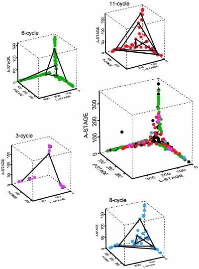
Although direct plots of the LMC vs. time, as in Fig. 2, contain the essence of the episode-identification procedure, it is revealing to see the cycle episodes as they are reflected in the data themselves. In Fig. 3, we plot the data the same way we presented the model-predicted cycles in Fig. 1. The large graph at the center of the figure shows all the data, and the surrounding graphs show the data decomposed into the four model-predicted cycles. The characteristic patterns drawn from both the continuous- and discrete-state models make up the anatomy of the chaotic attractor as it is seen in the experimental data.

Fig. 3.

Cycle episodes in the data. The central graph is a phase-space plot of all data. Data points belonging to identified cycle episodes (see Fig. 2) are red, green, and magenta, corresponding to Figs. 1 and 2. In the surrounding graphs, data points corresponding to particular cycle episodes are isolated; some points are connected to indicate the temporal sequence. The black dots are data points not assigned to one of the model-predicted cycles.

In addition to the patterns associated with the chaotic attractor and its discrete-state analogue, the influence of the continuous-state model's unstable equilibrium is clearly seen in these data (25, 42). Applied to an equilibrium, or 1-cycle, the LMC is nothing more than the distance to the equilibrium. Fig. 4 shows the passage of the data through the vicinity of this unstable equilibrium (a so-called fly-by of the unstable equilibrium). Notice that during this interval the LMCs of the other model-predicted cycles are tightly plaited, as seen in Fig. 2.

Fig. 4.

Equilibrium fly-by. (A) L-stage time-series data. (B) Distances from data points to the unstable equilibrium of the deterministic continuous-state model (Eq. 1). The equilibrium fly-by is indicated by arrows. Note that the LMCs for other cycles (Fig. 2) are tightly plaited during the fly-by.

The models expressed in Eqs. 1 and 2 are deterministic and thus themselves cannot generate the mixture of cycle patterns seen in the data. We examined the stochastic model (Eq. 3) to verify that it is capable of generating patterns similar to those observed. We computed LMCs for orbits of the stochastic model. Typical results are shown in Fig. 5. Note that, although the particular sequence of cycle episodes in any stochastic realization differs from that in the data, the model shows a similar mixture of cycle episodes.

Fig. 5.

Lag metrics in a stochastic realization. The same procedure used to generate Fig. 2 has been applied to a realization of the discrete-state stochastic model (Eq. 3). (A) L-stage time-series data. (B–F) LMC with respect to the model-predicted cycles: continuous-state model saddle 11-cycle (B); discrete-state model 8-cycle (C); discrete-state model 6-cycle (D); discrete-state model 3-cycle (E); and continuous-state model unstable equilibrium (1-cycle) (F). (G) Intervals identified as cycle episodes are depicted (see Appendix for a description of the procedure we used). (H) L-stage time-series data as in A, with 11-, 6-, and 3-cycle episodes identified in red, green, and magenta corresponding to Figs. 1, 2, 3.

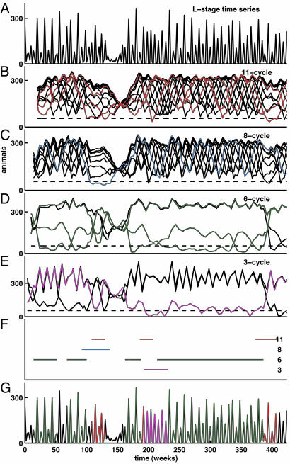
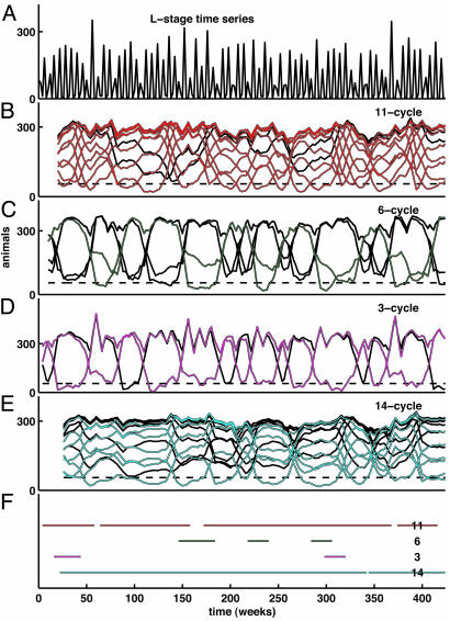
It is important to note that the mixture of patterns generated by the stochastic model (Eq. 3) depends markedly on the habitat size, V. In particular, as the parameter V is increased, the attractors of the discrete-state deterministic model (Eq. 2) change in complicated ways despite the fact that the chaotic attractor of the continuous-state model (Eq. 1) is unchanged (30, 31). In contrast to the case for which V = 1, when V = 3 (corresponding to a 60-g habitat), the discrete-state deterministic model (Eq. 2) has but one attractor: a 14-cycle. Correspondingly, the stochastic model (Eq. 3) displays a less-rich mixture of recurrent patterns in this case (Fig. 6). Indeed, the 14-cycle is overwhelmingly in evidence. Moreover, for reasons discussed in ref. 30, the 11-cycle embedded in the chaotic attractor of Eq. 1 is more prominent at the larger habitat size. The implication for biologists is that an experiment or observation can uncover very different images of the underlying chaotic dynamics depending on the scale of the system.

Fig. 6.

Cycle episodes in a stochastic orbit at V = 3. The same procedure used to generate Fig. 2 has been applied to a realization of the discrete-state stochastic model (Eq. 3) with habitat size V = 3. (A) L-stage time-series data. (B–E) LMC with respect to the model-predicted cycles: continuous-state model saddle 11-cycle (B); discrete-state model 6-cycle (which exists for V = 1 but not at V = 3) (C); discrete-state model 3-cycle (which again exists at V = 1 but not at V = 3) (D); and discrete-state model 14-cycle (which exists at V = 3 but not at V = 1) (E). (F) Intervals identified as cycle episodes (see Appendix) are depicted. For the 14-cycle, we used the more stringent K = 15.

Discussion

Other authors have noted transient periodicity in data. Lathrop and Kostelich (32) and So et al. (43) applied nonparametric nonlinear forecasting techniques to long series of data from the Belousov–Zhabotinskii reaction and neuronal electrophysiological recordings, respectively, and found evidence for saddle cycles in the data. Schaffer et al. (27) observed similarities between saddle cycles predicted by an epidemiological model and historical measles case-report data. The present study builds on these successes and goes further to show quantitative agreement between model-predicted periodic behaviors and experimental data. Two developments have made this possible.

The first is an appreciation for the dynamical effects of individuation, system size, and the stochastic nature of demographic events. Mathematically, discreteness of individuals gives state space a granularity that alters and diminishes the set of possible dynamical behaviors. The set of behaviors depends on the degree of state-space granularity, which in turn depends on the system size (30, 44). In such a system, stochasticity acts not to obliterate but to reveal the deterministic signal through the continual reexcitation of transients.

The second is the development of new techniques for identifying subtle transient patterns in relatively short time series. The LMC, introduced in the present contribution, is a direct comparison between data and model-predicted cycles, designed to detect complex and episodic temporal patterns. Naturally, the noise level and time-series length impose limits on the resolution of this tool. Similarly, the noise intensity sets the maximum resolvable cycle period (cf. refs. 38 and 45). Thus, although the 3-cycle and 6-cycle are distinguishable in the data presented here, it would be futile to attempt to distinguish the model-predicted 11-cycle from closely related cycles of higher period, such as its period-doubled descendant cycles of periods 22, 44, 88, etc., which are also present in the deterministic dynamics of Eq. 1.

Our results shed additional light on the manner in which deterministic chaos can be expected to leave its mark on population data. In particular, it is the transient but recurrent cyclic patterns generated by chaotic attractors and their discrete-state analogues, woven together by stochasticity, that distinguish chaos as it is manifested in noisy, discrete-state population systems. The unambiguous identification of chaos or, more generally, deterministic signals, in natural populations will remain a difficult challenge, in part because ecological time series tend to be short. An understanding of the mode in which complex dynamics are expressed in real data is therefore essential for continued progress.

Appendix

Experimental Protocol. The experiment reported in refs. 23–25 was designed to test for a predicted sequence of changes in dynamical behavior as a demographic parameter was varied. We experimentally set the adult mortality rate at μ_a = 0.96 and manipulated the adult recruitment rate such that the number of new adults at time t would equal P_t exp(-c_pa A_t) with values of c_pa set at 0.00, 0.05, 0.10, 0.25, 0.35, 0.50, and 1.00.

There was also an unmanipulated control treatment. Twentyfour cultures of the RR strain of the flour beetle Tribolium castaneum (Herbst) were initiated with 250 L-stage insects, 5 P-stage animals, and 100 A-stage sexually mature young adults. Three populations were assigned randomly to each of the eight treatments. Each population was maintained in a half-pint (237-ml) milk bottle with 20 g of standard medium and kept in an unlighted incubator at 32°C. Every 2 weeks the L, P, and A stages were counted and returned to fresh medium, and dead adults were counted and removed. In this article, we present data for one replicate of the c_pa = 0.35 treatment, maintained under the laboratory protocol mentioned above for 424 weeks (8.1 years) of biweekly counts, or ≈70 generations of flour beetles.

Parameter Estimates. The model parameters were estimated on the basis of the first 80 weeks of data, as described in ref. 24. Point estimates (95% confidence intervals) of the parameter values are b = 10.45 (10.04,10.77), μ_l = 0.2000 (0.1931,0.2068), c_ea = 0.1310 (0.01285,0.01340), and c_el = 0.01731 (0.01611,0.01759). For the variance–covariance matrix, we used the following values estimated in ref. 24: Σ₁₁ = 2.332, Σ₂₂ = 0.2374, Σ₁₂ = Σ₂₁ = 0.0071. Dennis et al. (24) concluded that the populations were strongly influenced by chaotic dynamics.

LMC. Given a length-N sequence of data vectors, , and a model T-cycle, , we define the LMC of d and m at lag s and time t by the formula

where ∥x∥ = |x₁| + |x₂| + |x₃| is a norm on the three-dimensional state space. In Figs. 2 and 4, 5, 6, we plotted LMC(s, t) against t directly. To aid in the interpretation of these graphs, one can fix a threshold number of animals θ and threshold duration K, picking out as T-cycle episodes those intervals [t₁, t₂] for which (i) there is a single phase s such that LMC(s, t) < θ, for all t ∈ [t₁, t₂] and (ii) t₂ - t₁ ≥ K - T. That is, we identify as T-cycle episodes those intervals for which the lowest strand of the LMC braid remains low for a long time. The effects of varying θ and K are immediately evident from examination of the LMC braid plots.

References

- 1.May, R. M. (1976) Nature 261, 459-467. [DOI] [PubMed] [Google Scholar]
- 2.Schaffer, W. M. (1984) Am. Nat. 124, 798-820. [Google Scholar]
- 3.Schaffer, W. M. (1988) in Evolution of Life Histories of Mammals, ed. Boyce, M. S. (Yale Univ. Press, New Haven, CT), pp. 313-350.
- 4.Sugihara, G., Grenfell, B. & May, R. M. (1990) Philos. Trans. R. Soc. London B 330, 235-251. [DOI] [PubMed] [Google Scholar]
- 5.Sugihara, G. & May, R. M. (1990) Nature 344, 734-741. [DOI] [PubMed] [Google Scholar]
- 6.Hanski, I., Turchin, P., Korpimaki, E. & Henttonen, H. (1993) Nature 364, 232-235. [DOI] [PubMed] [Google Scholar]
- 7.Hastings, A., Hom, C. L., Ellner, S., Turchin, P. & Godfray, H. C. J. (1993) Annu. Rev. Ecol. Syst. 24, 1-33. [Google Scholar]
- 8.Wilson, H. B. & Rand, D. A. (1993) Proc. R. Soc. London Ser. B 253, 239-244. [Google Scholar]
- 9.Grenfell, B. T., Kleczkowski, A., Ellner, S. P. & Bolker, B. M. (1994) Philos. Trans. R. Soc. London A 348, 515-530. [Google Scholar]
- 10.Tong, H., ed. (1995) Chaos and Forecasting (World Scientific, Singapore).
- 11.Ellner, S. P., Bailey, B. A., Bobashev, G. V., Gallant, A. R., Grenfell, B. T. & Nychka, D. W. (1998) Am. Nat. 151, 425-440. [DOI] [PubMed] [Google Scholar]
- 12.Pool, R. (1989) Science 243, 25-28. [DOI] [PubMed] [Google Scholar]
- 13.Stone, L. (1992) Proc. R. Soc. London Ser. B 250, 77-81. [Google Scholar]
- 14.Turchin, P. (1993) Oikos 68, 167-172. [Google Scholar]
- 15.Falck, W., Björnstad, O. N. & Stenseth, N. C. (1995) Proc. R. Soc. London Ser. B 261, 159-165. [Google Scholar]
- 16.Falck, W., Björnstad, O. N. & Stenseth, N. C. (1995) Proc. R. Soc. London Ser. B 262, 363-370. [Google Scholar]
- 17.Turchin, P. (1995) Proc. R. Soc. London Ser. B 262, 357-361. [Google Scholar]
- 18.Perry, J. N., Smith, R. H., Woiwod, I. P. & Morse, D. R., eds. (2000) Chaos in Real Data: The Analysis of Non-Linear Dynamics from Short Ecological Time Series (Kluwer, Dordrecht, The Netherlands).
- 19.Turchin, P. & Ellner, S. P. (2000) Ecology 81, 3099-3116. [Google Scholar]
- 20.Zimmer, C. (1999) Science 284, 83-86. [Google Scholar]
- 21.Björnstad, O. N. & Grenfell, B. T. (2001) Science 293, 638-643. [DOI] [PubMed] [Google Scholar]
- 22.Dennis, B., Desharnais, R. A., Cushing, J. M., Henson, S. M. & Costantino, R. F. (2003) Oikos 102, 329-340. [Google Scholar]
- 23.Costantino, R. F., Desharnais, R. A., Cushing, J. M. & Dennis, B. (1997) Science 275, 389-391. [DOI] [PubMed] [Google Scholar]
- 24.Dennis, B., Desharnais, R. A., Cushing, J. M., Henson, S. M. & Costantino, R. F. (2001) Ecol. Monogr. 71, 277-303. [Google Scholar]
- 25.Cushing, J. M., Costantino, R. F., Dennis, B., Desharnais, R. A. & Henson, S. M. (2003) Chaos in Ecology: Experimental Nonlinear Dynamics, Theoretical Ecology Series (Academic, London), Vol. 1.
- 26.Rohani, P. & Earn, D. J. D. (1997) Trends Ecol. Evol. 12, 171. [DOI] [PubMed] [Google Scholar]
- 27.Schaffer, W. M., Kendall, B. E., Tidd, C. W. & Olsen, L. F. (1993) IMA J. Math. Appl. Med. Biol. 10, 227-247. [DOI] [PubMed] [Google Scholar]
- 28.Kendall, B. E., Schaffer, W. M., Olsen, L. F., Tidd, C. W. & Jorgensen, B. L. (1993) in Predictability and Nonlinear Modelling in Natural Sciences and Economics, eds. Grassman, J. & van Straten, G. (Kluwer, Dordrecht, The Netherlands), pp. 184-203.
- 29.Turchin, P. (2003) Complex Population Dynamics: A Theoretical/Empirical Synthesis, Monographs in Population Biology. (Princeton Univ. Press, Princeton), Vol. 35.
- 30.Henson, S. M., Costantino, R. F., Cushing, J. M., Desharnais, R. A., Dennis, B. & King, A. A. (2001) Science 294, 602-605. [DOI] [PubMed] [Google Scholar]
- 31.Henson, S. M., King, A. A., Costantino, R. F., Cushing, J. M., Dennis, B. & Desharnais, R. A. (2003) Proc. R. Soc. London Ser. B 270, 1549-1553. [DOI] [PMC free article] [PubMed] [Google Scholar]
- 32.Lathrop, D. P. & Kostelich, E. J. (1989) Phys. Rev. A At. Mol. Opt. Phys. 40, 4028-4031. [DOI] [PubMed] [Google Scholar]
- 33.Kendall, B. E., Schaffer, W. M. & Tidd, C. W. (1993) Phys. Lett. A 177, 13-20. [Google Scholar]
- 34.King, A. A. & Schaffer, W. M. (1999) J. Math. Biol. 39, 439-469. [DOI] [PubMed] [Google Scholar]
- 35.Cushing, J. M., Henson, S. M., Desharnais, R. A., Dennis, B., Costantino, R. F. & King, A. (2001) Chaos Solitons Fractals 12, 219-234. [Google Scholar]
- 36.So, P., Ott, E., Schiff, S. J., Kaplan, D. T., Sauer, T. & Grebogi, C. (1996) Phys. Rev. Lett. 76, 4705-4708. [DOI] [PubMed] [Google Scholar]
- 37.So, P., Ott, E., Sauer, T., Gluckman, B. J., Grebogi, C. & Schiff, S. J. (1997) Phys. Rev. E Stat. Phys. Plasmas Fluids Relat. Interdiscip. Top. 55, 5398-5417. [Google Scholar]
- 38.Dhamala, M, Lai, Y. C. & Kostelich, E. J. (2000) Phys. Rev. E Stat. Phys. Plasmas Fluids Relat. Interdiscip. Top. 61, 6485-6489. [DOI] [PubMed] [Google Scholar]
- 39.Xu, D, Li, Z, Bishop, S. R. & Galvanetto, U. (2002) Pattern Recognit. Lett. 23, 245-252. [Google Scholar]
- 40.Domokos, G. & Scheuring, I. (2002) Science 297, 2163. [DOI] [PubMed] [Google Scholar]
- 41.King, A. A., Desharnais, R. A., Henson, S. M., Costantino, R. F., Cushing, J. M. & Dennis, B. (2002) Science 297, 2163.12351754 [Google Scholar]
- 42.Cushing, J. M., Dennis, B., Desharnais, R. A. & Costantino, R. F. (1998) J. Anim. Ecol. 67, 298-306. [Google Scholar]
- 43.So, P., Francis, J. T., Netoff, T. I., Gluckman, B. J. & Schiff, S. J. (1998) Biophys. J. 74, 2776-2785. [DOI] [PMC free article] [PubMed] [Google Scholar]
- 44.Binder, P.-M. & Okamoto, N. H. (2003) Phys. Rev. E Stat. Phys. Plasmas Fluids Relat. Interdiscip. Top. 68, 046206. [Google Scholar]
- 45.Dhamala, M, Lai, Y. C. & Kostelich, E. J. (2001) Phys. Rev. E Stat. Phys. Plasmas Fluids Relat. Interdiscip. Top. 64, 056207. [DOI] [PubMed] [Google Scholar]