Multi-class maximum likelihood symmetry determination and motif reconstruction of 3-D helical objects from projection images for electron microscopy

Abstract

Many micro- to nano-scale 3-D biological objects have a helical symmetry. Cryo electron microscopy provides 2-D projection images where, however, the images have low SNR and unknown projection directions. The object is described as a helical array of identical motifs, where both the parameters of the helical symmetry and the motif are unknown. Using a detailed image formation model, a maximum likelihood estimator for the parameters of the symmetry and the 3-D motif based on images of many objects and algorithms for computing the estimate are described. The possibility that the objects are not identical but rather come from a small set of homogeneous classes is included. The first example is based on 316 128×100 pixel experimental images of Tobacco Mosaic Virus, has one class, and achieves 12.40Å spatial resolution in the reconstruction. The second example is based on 400 128 × 128 pixel synthetic images of helical objects constructed from NaK ion channel pore macromolecular complexes, has two classes differing in helical symmetry, and achieves 7.84Å and 7.90Å spatial resolution in the reconstructions for the two classes.

I. Introduction

A wide variety of biological objects have a helical symmetry and can be visualized in the transmission electron microscope with cryogenic specimen preparation (cryo EM). The resulting image is a 2-D projection, with an unknown projection direction, of the 3-D distribution of electron scattering intensity of the object. Because of the sensitivity of the object to the electron beam, the usual approach is to fuse information from one image of each of many identical objects. In addition to the unknown direction of the projection, these problems are complicated by failure to know the parameters of the helical symmetry that is present and by the low SNR of the images. In this paper a statistical model, maximum likelihood (ML) estimator, and a variety of generalized expectation maximization algorithms are proposed for simultaneously determining the parameters of the helical symmetry and the 3-D electron scattering intensity when images show objects that come from one or more homogeneous classes where, if more than one class is present, different symmetry parameters and/or different electron scattering intensity distributions for the repeat element of the object are jointly determined for each class.

Helical symmetry arises in biological objects when a macromolecule or macromolecular complex, the so-called motif, is repeated in a helical array. The motif for Tobacco mosaic virus (TMV) is shown in Figure 1(a) and a helical array is shown schematically in Figure 1(b). Because helical arrays are periodic in one of the three coordinates, conventionally called the z coordinate, the 3-D Fourier transform is impulsive in the corresponding k_z coordinate of Fourier space and the function of k_x and k_y that multiplies the impulse is called a layer plane. The situation for the 2-D image provided by an electron microscope is similar but now, in the appropriate coordinate system, the function that multiples the impulse is a function of only one coordinate rather than two coordinates and is called a layer line. An image showing the magnitude of the 2-D Fourier transform of an ideal image of TMV, where every column of pixels is either zero or the magnitude of a layer line, is shown in Figure 1(c).

Fig. 1.

Helices. Panel (a): The motif of TMV. Panel (b): A schematic showing the construction of a helical array of motifs. Please note that the motif rotates at the same time as the location of the motif both rotates and translates. Panel (c): The magnitude of the 2-D Fourier transform of synthetic TMV constructed from the motif of Panel (a) showing multiple layer lines where the impulsive coordinate is the horizontal coordinate and the layer line is shown as pixel intensities in the vertical direction. (Combined from Ref. [1, Figures 1(a), 3(a), and 6(c)]).

The range of biological objects that have helical symmetry is large [2]. At the molecular level, examples include actin [3], [4], tubulin and microtubules [5], and flagellin and flagellum [6]. At the macromolecular complex level, a large number of viruses exhibit helical symmetry, including viruses in the genus Tobamovirus which includes the species Tobacco mosaic virus used as an example in this paper. In addition, some membrane-based components of cells can be induced to form tubular objects in which the many copies of the same membrane protein form a helical array (e.g., Ca²⁺-ATPase of the Sarcoplasmic reticulum [7] and nicotinic acetylcholine receptor of the electric organ of the Torpedo electric ray [8]). Finally, synthetic lipid nanotubes [9] can be used as substrates on which to form helical arrays of protein molecules (e.g., Streptavidin [10], Perfringolysin O [11], and IgG and Transducin [12]). Planar lipid layers can also be used as substrates resulting in 2-D crystals with various space groups, but the advantage of the nanotubes and helical arrays is that a complete set of data can be recorded without the necessity of tilting the specimen in the electron microscope.

Corresponding to the importance of the problem, there are multiple algorithms and software systems designed to determine the parameters of the helical symmetry, determine the orientation of each image, and compute a reconstruction including IHRSR [2], [13], Phoelix [14], Ruby-helix [15], the Brandeis Helical Package [16], the MRC Image Processing Programs [17], Spider and Web [18], and the Stokes Lab Procedures¹. With the exception of IHRSR, the underlying mathematics of these algorithms is a Fourier-Bessel series for the 3-D distribution electron scattering intensity [19] described in reciprocal space (i.e., Fourier space) while the approach of IHRSR is based on a voxel representation in real space (i.e., Image space). Furthermore, if the objects come from more than one class, all of these approaches must first label all images with respect to what class of object is shown and then separately process the images which share the same class label. The labeling process can be challenging because only a noisy unoriented 2-D projection of the 3-D object is shown in an image.

The 3-D electron scattering intensity of an object with helical symmetry can be described as a helical array of identical 3-D subobjects called motifs. The approach in this paper differs from the approaches of the previous paragraph because the underlying mathematics is a description of the electron scattering intensity of a single motif [1]. From a mathematical point of view, there is not a unique motif for an object with helical symmetry. However, from a biological point of view, there usually is a natural definition of the motif because the biological object is constructed from macromolecules and the natural motif is the smallest collection of such molecules which, when placed in a helical array, create the object. Focusing on the motif has several potential advantages. First, if the motif is known or hypothesized to have a symmetry [20], that symmetry can easily be incorporated into the reconstruction. Second, if the helical objects are not homogeneous, then, using a multi-class maximum likelihood approach, it is possible to separately consider whether the same motif forms helices of different symmetries (e.g., due to changing diameter of a lipid tube substrate) or multiple motifs occur in multiple different symmetries (e.g., due to a protein molecule that has more than one conformation when packed in a helix), etc. Third, though it is beyond the scope of this paper, the motif mathematics can be generalized to include variability in the translation and rotation present between adjacent motifs in the helical array leading to a natural description of random helices as has been useful previously in other biophysical structure problems [21].

With the exception of IHRSR, the algorithms listed above process reciprocal-space images. The choice of applying the ideas of this paper to images in real versus reciprocal space is determined by the definition of the matrix L (Eq. 1). The formulas (Eq. 3) and computations (Section X) of this paper are for processing reciprocal-space images. In order to process real-space images, it is necessary to compute the 2-D inverse Fourier transform of Eq. 3 in order to determine the values of the matrix L. The reason that we have used reciprocal-space images is that it appears difficult to do this computation symbolically. While many algorithms allow the averaging of images in order to increase SNR, the algorithms described in this paper consider each image separately. Because the helical symmetry includes periodicity in one dimension, an ideal reciprocal-space image is zero except for impulsive so-called layer lines. While it is possible to consider algorithms that extract and process layer lines from reciprocal-space images, the algorithms described in this paper in fact process all pixels in the reciprocal-space images. Finally, an important feature of the algorithm described in this paper is that it can process images where the object did not lie in the plane perpendicular to the beam in the microscope, i.e., objects with so-called “out-of-plane tilt”.

In cylindrical coordinates, a function ρ(r, φ, z) has a screw symmetry in the z direction if and only if ρ(r, φ, z) = ρ(r, φ + φ₀, z + z₀) for specific values of φ₀ ∈ [0, 2π) and z₀ ∈ IR. A helical symmetry is stricter since it constrains φ₀ and z₀ by requiring that ρ be periodic in z. Let c denote the fundamental period. Then there must be integers u and v such that uz₀ = c and uφ₀ = v2π or, equivalently, z₀ = c/u and φ₀ = v2π/u where, in addition, u and v are relatively prime in order that c is the fundamental period. In this paper we focus on helical symmetry although much the same approach can be applied to screw symmetry. In particular, by increasing u, v, and c, any screw symmetry can be approximated by a helical symmetry with a large period.

Most of the engineering literature that describes work on 3-D reconstruction problems for cryo EM concerns single-particle cryo EM for spherical particles [22]–[30]. Helical problems are more difficult because the parameters of the helical symmetry are not known a priori. However, helical problems are also easier because a single image provides several views of the motif, in relative directions determined by the helical symmetry, though the views are overlapping in the resulting image. The work described in this paper and all of the helical algorithms referenced previously process an image of an object with helical symmetry by first dividing the image into subimages in order to ameliorate nonidealities in the object. By processing subimages, helical problems more closely resemble spherical problems.

In summary, the goal of this paper is to describe a maximum likelihood estimator and algorithms for its computation that jointly determines multiple motif distributions of electron scattering intensity and multiple helical symmetry parameters based on unlabeled images that are randomly selected from homogeneous classes. As a part of achieving this goal, the estimator uses detailed models of the image formation process that include a Contrast Transfer Function and a complete 6 degrees of freedom for the position of the object in the microscope.

II. Mathematical notation

Let (IR) denote the integers (reals). Let x ∈ IR³ (χ ∈ IR²) denote position in the 3-D real-space cube (2-D real-space image). Let k ∈ IR³ (κ ∈ IR²) denote the corresponding frequency vector in reciprocal space where the 3-D Fourier transform is defined by P(k) = ∫ρ(x) exp(−i2πk^T x)d³x and similarly for the 2-D case. Let k = |k| and κ = |κ|. Let I_n denote the n × n identity matrix. Let N(m, Q) denote the multivariate Gaussian probability density function (pdf) with mean m and covariance matrix Q.

III. Image formation model: Deterministic

The motif is described by a weighted linear combination of basis functions so that estimating the motif is equivalent to estimating the weights. The basis functions used are a complete orthonormal set [30, Eqs. 2–3]. The image formation model includes the transformation from weights to motif, the transformation from motif to helix, the positioning of the helix in the microscope, the 2-D projection of the 3-D helix by the microscope, the convolution of the projection with the Contrast Transfer Function (CTF) of the microscope, and the windowing of the infinitely long image of the helix to a finite image. For the effect of the microscope, please see, for example, Refs. [31], [32] [33] [34, p. 874]. The spacing between the zero crossings of the CTF is linear in the amount that the microscope is defocused and therefore is under user control. Other aspects of the CTF, such as the decay of the envelope of the CTF due to factors such as beam coherence and the mixture of amplitude versus phase contrast are not easily under user control.

The total transformation from weights to finite image is linear in the weights. Therefore, if y denotes an image arrayed as a vector (dimension N_y) and d denotes the weights d_l,m,p arrayed as a vector (dimension N_d), then

$$y=L(s)d$$ (1)

where the transformations are different for real versus reciprocal space and where s denotes all of the parameters of the transformation. In the remainder of this paper, y is always the reciprocal-space image. The parameters are listed in Table I and described in the following paragraph.

TABLE I.

Parameters in L (Eq. 1). “?” indicates a parameter for which the value is to be determined from the images. Additional parameters not in L are only d (containing all the d_l,m,p), which also appears in Eq. 1, and Q, which is the covariance of the noise w in Eq. 4.

	Parameter	Example 1 TMV	Example 2 Ion channel pore
Motif	r1 (Å)	0.0	?
	r2 (Å)	60.367	?
	lmax	6	12 or 8
	pmax	10	6 or 5
Rotation of motif to helix coordinates†	αH (rad)	0.0	0.0
	βH (rad)	0.0	π/2
	γH (rad)	0.0	0.0
Helical symmetry‡	c(Å)	?	80.0 or 130.0
	u	?	?
	v	?	?
	rH (Å)	56.484	?
Rotation of helix to microscope coordinates¶	αL (rad)	?	?
	βL (rad)	?	?
	γL (rad)	?	?
Translation	xL1(Å)	?	?
	xL2 (Å)	?	?
CTF§	Δf(Å)	8 or 20 × 103	8 or 20 × 103
	Cs (Å)	2 × 107	2 × 107
	λ(Å)	0.0336	0.0336
	Famp	0.2	0.2
	B(Å2)	100.0	100.0
Image sampling	N	128	128
	Δ (Å)	2.263	1.88

^†The 3 × 3 rotation matrix R_H is specified by Euler angles (α_H, β_H, γ_H).

^‡An alternative to c, u, and v are z₀ and φ₀ defined by z₀ = c/u and φ₀ = 2πv/u (Section III).

^¶The 3 × 3 rotation matrix R_L is specified by Euler angles (α_L, β_L, γ_L).

^§The CTF (Contrast Transfer Function) is computed by the unnumbered formula on p. 874 of Ref. [34] where Δf is the deviation from Gaussian focus, C_s is the coefficient of spherical aberration, λ is the electron wavelength, F_amp is the fractional amplitude contrast, and B is the decay.

The motif is described in the so-called motif coordinate system. The coordinate system is important primarily in cases where the motif is known to have a 3-D symmetry (e.g., Section X-B). In this coordinate system, the 3-D distribution of electron scattering intensity of the motif, denoted by ρ(x) and P(k) in real and reciprocal space, respectively, is described by a truncated orthonormal expansion where the weights in the expansion are denoted by d_l,m,p. In the computations presented in Section X, the expansion for P is written in spherical coordinates and the basis functions are products of angular and radial functions,

$$P(\mathbf{k})=\sum _{l=0}^{l_{max}}\sum _{m=0}^{2l}\sum _{p=1}^{p_{max}}{(-i)}^l{d}_{l,m,p}{H}_{l,p}(k){\mathrm{\Psi }}_{l,m}(\theta ,\phi ),$$ (2)

where H_l,p is related to spherical Bessel functions [30] and Ψ_l,m is a linear combination of Y_l,m′ where Y_l,m′ (m′∈ {−l, …, +l}) are spherical harmonics. As shown in Eq. 2, the angular dependence is indexed with nonnegative integers l and m where the range of l is infinite but in practice truncated at l_max and the radial dependence is indexed with nonnegative integers l and p where the range of p is also infinite but in practice truncated at p_max. In real space, the radial basis functions are nonzero in the spherical shell of inner radius r₁ and outer radius r₂. The motif is then rotated into the orientation that it takes in the object by a rotation matrix, denoted by R_H and described by Euler angles α_H, β_H, γ_H. The helix is described in object coordinates in which the helical axis is the z axis. The helical object is constructed as if it was built one motif at a time: the first rotated motif is translated to location (r_H, 0, 0)^T in object coordinates where r_H + r₂ is the radius of the helical object. The other motifs are added to the helix by translation and rotation of the first motif. For the nth motif (n ∈ ), the translation is by nz₀ in the z direction and the rotation is by nφ₀ around the z axis where z₀ and φ₀ are defined as functions of c, u, v by z₀ = c/u and φ₀ = 2πv/u and the parameters c, u, v are the period of the helical object, the number of motifs per period, and the number of turns per period, respectively. The helical object in object coordinates is then rotated and translated to laboratory coordinates in the microscope. The rotation matrix R_L is described by Euler angles α_L, β_L, γ_L and the translation is described by (x_L1, x_L2, 0)^T where the projection direction in the microscope is the z direction in laboratory coordinates and therefore the third component of the translation can be taken equal to 0 without loss of generality. In the spatial frequency domain, the projection image is modified by the Contrast Transfer Function (CTF) [34] which has parameters Δf, C_s, λ, F_amp, and B. The dimension of the square pixel is Δ and the number of pixels along the helical axis in the image is N.

The 2-D Fourier transform of the infinite image (i.e., the reciprocal-space infinite image) is denoted by Σ_∞(κ) and is related to the weights d_l,m,p of the orthonormal expansion of the 3-D distribution of electron scattering intensity and the other parameters by ${\mathrm{\sum }}_{\infty }(\mathit{\kappa })=[{\sum }_{n=-\infty }^{+\infty }\delta ({\kappa }_1-{\kappa }_{2}tan{\gamma }_L+n/(csin{\beta }_{L}cos{\gamma }_L))]S({\kappa }_1,{\kappa }_2)$ (please see [1], [35] for the definition of S). This expression is purely impulsive due to the periodicity of the ideal helix, where the impulse at the location where κ₁ and κ₂ satisfy κ₁ − κ₂ tan γ + n/(c sin β_L cos γ_L) = 0 is the nth layer line.

An experimental image is of finite length and therefore its Fourier transform has layer lines of finite width. In order to model the finite width of the layer lines, the finite real space image, denoted by σ(χ) with 2-D Fourier transform denoted by Σ(κ), is described as the product of a binary mask, denoted by μ(χ) with 2-D Fourier transform denoted by M(κ), and the infinite image, denoted by σ_∞(χ) with 2-D Fourier transform Σ_∞(κ). By preliminary processing of the micrograph, the images of the objects have γ_L near 0, i.e., the projection of the long axis of the helix is approximately in the χ₁ direction. Therefore it does not matter whether the mask is finite or infinite in extent in the χ₂ direction and infinite extent leads to simpler equations. Based on these considerations, the definition of μ(χ) is μ(χ) = 1 if |χ₁/(NΔ)| ≤ 1/2 and = 0 otherwise where N and Δ were defined previously. The definition of μ(χ) implies M(κ) = N Δ sinc(NΔκ₁). Therefore σ(χ) = σ_∞(χ)μ(χ) which implies that Σ(κ) = Σ_∞(κ) * M (κ). The formula for Σ_∞ is derived in Refs. [1], [35]. For the case R_H = I₃, the formula for Σ is

$$\begin{array}{l}\mathrm{\sum }(\mathit{\kappa })=\sum _{n=-\infty }^{+\infty }\frac{sin[\pi N\mathrm{\Delta }({\kappa }_1-{\kappa }_{\ast }(n,{\kappa }_2))]}{\pi ({\kappa }_1-{\kappa }_{\ast }(n,{\kappa }_2)))}\\ \times \frac{G({\kappa }^{\prime })}{csin{\beta }_{L}cos{\gamma }_L}exp\left(-i2\pi [{\kappa }_{\ast }(n,{\kappa }_2)x_{L_1}+{\kappa }_2{x}_{L_2}]\right)\\ \times \left[\sum _{l=0}^{\infty }\sum _{m=0}^{2l}\sum _{p=1}^{\infty }{d}_{l,m,p}{(-i)}^l{H}_{l,p}({\kappa }^{\prime })\right[\sum _{n^{\prime }=0}^{u-1}exp(-i2\pi \\ \times [n^{\prime }{z}_0{\tau }_3^{\prime }(n,{\kappa }_2)+r_H{\tau }_1^{\prime }(n,{\kappa }_2,n^{\prime })]){\mathrm{\Psi }}_{l,m}({\theta }^{\prime },{\phi }^{\prime })]]\end{array}$$ (3)

where κ = (κ₁, κ₂)^T, κ = |κ|, G(κ) is the CTF, and ${\kappa }^{\prime }=\sqrt{{[{\kappa }_{\ast }(n,{\kappa }_2)]}^2+{\kappa }_2^2}$, ${\theta }^{\prime }=arctan\left(\sqrt{{({\tau }_1^{\prime })}^2+{({\tau }_2^{\prime })}^2}/{\tau }_3^{\prime }\right),{\phi }^{\prime }=arctan({\tau }_2^{\prime }/{\tau }_1^{\prime })$, ${\tau }_1^{\prime }(n,{\kappa }_2,n^{\prime })={\kappa }_{\ast }(n,{\kappa }_2)[cos({\alpha }_L+n^{\prime }{\phi }_0)cos{\beta }_{L}cos{\beta }_{L}cos{\gamma }_L-sin({\alpha }_L+n^{\prime }{\phi }_0)sin{\gamma }_L]-{\kappa }_2[cos({\alpha }_L+n^{\prime }{\phi }_0)cos{\beta }_{L}sin{\gamma }_L+sin({\alpha }_L+n^{\prime }{\phi }_0)cos{\gamma }_L]$, ${\tau }_2^{\prime }(n,{\kappa }_2,n^{\prime })={\kappa }_{\ast }(n,{\kappa }_2)[sin({\alpha }_L+n^{\prime }{\phi }_0)cos{\beta }_{L}cos{\gamma }_L+cos({\alpha }_L+n^{\prime }{\phi }_0)sin{\gamma }_L]+{\kappa }_2[-sin({\alpha }_L+n^{\prime }{\phi }_0)cos{\beta }_{L}sin\gamma +cos({\alpha }_L+n^{\prime }{\phi }_0)cos{\gamma }_L]$, ${\tau }_3^{\prime }(n,{\kappa }_2)=-{\kappa }_{\ast }(n,{\kappa }_2)sin{\beta }_{L}cos{\gamma }_L+{\kappa }_{2}sin{\beta }_{L}sin{\gamma }_L$, and κ_*(n, κ₂) = κ₂ tan γ_L − n/(c sin β_L cos γ_L). For R_H ≠ I₃, the term Ψ_l,m(θ, φ) is replaced by Ψ_l,m(θ′, φ′) where θ′ and φ′ are the spherical coordinate angles of the vector R_Hτ′ where ${\mathit{\tau }}^{\prime }={({\tau }_1^{\prime },{\tau }_2^{\prime },{\tau }_3^{\prime })}^T$. The reason for the complexity of Eq. 3, and especially the τ intermediate variables, is that Eq. 3 applies for any orientation of the object in the microscope, as is described by the three Euler angles α, β, and γ. In particular, β ≠ π/2 is an object with so-called “out-of-plane tilt”. For the most simple orientation, where the z axis of the object becomes the x axis of the image, α_L = 0, β_L = π/2, and λ_L = 0, the trigonometric terms simplify resulting in ${\tau }_1^{\prime }(n,{\kappa }_2,n^{\prime })=-{\kappa }_{2}sin(n^{\prime }{\phi }_0),{\tau }_2^{\prime }(n,{\kappa }_2,n^{\prime })={\kappa }_{2}cos(n^{\prime }{\phi }_0),{\tau }_3^{\prime }(n,{\kappa }_2)=-{\kappa }_{\ast }(n,{\kappa }_2)$, and κ_*(n, κ₂) = −n/c.

Eq. 3 describes the inner product of a row of L (Eq. 1) with the vector of weights, d. Therefore the elements of L can be read from Eq. 3. While motifs can have internal symmetries (Section X-B), helices can also have additional global symmetries [36, Sections 7.2.1.(a) and 7.2.3.(a)]. As is described in [35], cyclic C_Ns and dihedral D_Ns symmetries can be incorporated in this approach.

Two aspects of the image formation model can reduce computation. First, since the image is real valued, its Fourier transform is conjugate symmetric and therefore only one half of the reciprocal-space pixels must be processed. Second, if the image size, image sampling rate, and helix period allow, there can be regions of essentially zero between the layer lines even with finite line widths. In such regions, corresponding rows of L can be approximated by 0.

IV. Statistical model and estimator

An additive Gaussian noise model with zero mean and known covariance matrix Q is used to describe the uncertainty in the pixels of the image [27], [30]. Therefore, the deterministic image formation equation (Eq. 1) is modified to

$$y=L(s)d+w$$ (4)

where w is the N(0, Q) noise. Since typical exposures are 100 electrons per pixel, a Gaussian model rather than a Poisson model is acceptable and the Gaussian model also includes other forms of image degradation such as fluctuations in the vitreous ice characteristics. Furthermore, a Gaussian model greatly simplifies the estimator calculations in Section VI for d, which is critical since the dimension of d is at least several hundred. The assumption of known covariance is replaced in practice by estimation of the covariance from areas of the real-space image in which no object is located.

The approach taken in this paper to estimator design is maximum likelihood (ML). From Eq. 4, the pdf on the image conditional on the values of all of the parameters is

$$p(y\mid {\alpha }_L,{\beta }_L,{\gamma }_L,x_{L_1},x_{L_2},u,v,c,r_H,d)=N(L({\alpha }_L,{\beta }_L,{\gamma }_L,x_{L_1},x_{L_2},u,v,c,r_H)d,Q)(y).$$ (5)

Listed in Table I and used in Eq. 5 are a total of 23 parameters plus the unknown weights d_l,m,p. Each parameter can be treated as known, unknown but deterministic, or random with known a priori pdf (possibly including hyperparameters although hyperparameters do not occur in this paper). All of the unknown but deterministic parameters are estimated by ML. For the random with known a priori pdf parameters, the parameters could be estimated, e.g., by maximum a posteriori estimation, or simply integrated out of the likelihood function using the a priori pdf. In the problem formulation of this paper, these parameters are integrated out of the likelihood function and for that reason are called nuisance parameters. The remainder of this paragraph explains the treatment of each parameter. The motif parameters r₁, r₂, l_max, and p_max; the R_H rotation parameters α_H, β_H, γ_H; the CTF parameters Δf, C_s, λ, F_amp, and B; and the image sampling parameters N and Δ are assumed to be known and are therefore not estimated. The parameters of greatest interest to biologist users are d, u, v, c, and r_H because knowing these parameters is necessary and sufficient to reconstruct the 3-D helical object. The parameters u and v are relatively prime positive integers so describing a probability mass function (pmf) is difficult. Therefore they are treated as unknown but deterministic and estimated by ML. The parameter d is a high dimensional (> 10²) real-valued vector of weights for the orthonormal expansion description of the motif so describing a pdf is difficult. Therefore d is also treated as unknown but deterministic and estimated by ML. The parameters c and r_H can be estimated by preprocessing algorithms directly from the image. However, the estimates have errors that can be described by a pdf. Treating the result of preprocessing as a priori information provides a priori pdfs for c and r_H. Using the pdfs, the variables are treated as nuisance parameters which are not estimated. The parameters describing the location and the orientation of the object in the microscope, R_L (described by α_L, β_L, γ_L), x_L1, and x_L2 have natural pdfs that are described in Section VIII and are treated as nuisance parameters which are not estimated.

While all of the previous discussion and equations describe one image, the goal is to process many images jointly. Because many images are processed jointly, the potential exists that different images show different types of 3-D objects and therefore joint reconstruction and classification is important and we consider several types of different reconstruction and classification problems. For all the problems, the fundamental data is a set of electron micrographs, each displaying one or more objects where a typical object extends for typically 1500–3000Å in the direction of the helical axis.

One challenge is that biological objects do not exactly obey the laws of helical symmetry. There is an established set of techniques [14], [16], [37], [38] for extracting images of objects from the micrographs, rotating the images so that γ_L is nearly 0, and straightening the images of objects which are bent. In what follows, the images resulting from this process are referred to as “long images”. The long image is typically further divided, with boundaries perpendicular to the helical axis, into subimages referred to as “short images”. This allows artifacts to be excluded and decreases the effect of any residual deviation from straightness since the deviation is less apparent over shorter distances. Because the objects are typically somewhat distorted from helical symmetry (e.g., bent, stretched, compressed, and twisted), it is difficult to create pdfs relating the 5 degrees of positional information (α_L, β_L, γ_L, x_L1, x_L2) between adjacent short images. Therefore we assume that they are independent.

A second challenge is that the motif or the helical symmetry can change. A variety of types of changes, e.g., constant within a long image versus constant within only a short image, can be described in a unified manner by appropriate definitions for the class labels as is described in Appendix A.

The label is assumed to be a random variable with known a priori pmf which can vary from image to image. This is a relatively general formulation. For instance, if the different cases differ by large changes in the radius r_H or the period c, then the images can probably be classified accurately with respect to symmetry by preprocessing so the a priori pmf for an image might be concentrated on those label values corresponding to the preprocessor-estimated symmetry for that image. If preprocessing is possible but inaccurate, then less concentrated pmfs, which still vary from image to image, might be used. Finally, if preprocessing is not possible, a single pmf might be used for all images and, if nothing is known, that single pmf might be uniform.

Let i ∈ {1, 2, …, N_i} index the images, either the long or the short images, that carry the class label. Such images are referred to as indexed images. Let N_s(i) denote the number of short images extracted from the ith indexed image and let j ∈ {1, 2, …, N_s(i)} index the jth short image of the ith indexed image. There are two cases which are both of biological importance. If the 3-D object changes symmetry or motif along its length then so does the long image. In this case, the indexed images are the short images extracted from the long image and N_s(i) = 1. Alternatively, if the 3-D object has constant symmetry and motif along its length then so does the long image. In this case the indexed image is the long image and N_s(i) is in the order of 10 since approximately 10 short images are extracted from each long image. Let y_i,j denote the jth short image from the ith indexed image. Let y denote the vector composed of all the y_i,j vectors.

Let the number of classes be denoted by N_η and let η_i ∈ {1, 2, …, N_η} denote the class label for the ith indexed image. The symbol η is used in two ways: as a label when the identity of the image to which the label applies is not relevant and to denote the collection of all labels, i.e., η = (η₁, η₂, …, η_Ni).

Let z_i,j (i ∈ {1, 2, …, N_i} and j ∈ {1, 2, …, N_s(i)}) be the nuisance parameters which effect only the jth short image from the ith indexed image. In the work described in this paper, this definition of z_i,j implies that z_i,j = (α_L, β_L, γ_L, x_L1, x_L2)_i,j. Let z_i be the nuisance parameters which effect only the ith indexed image, i.e., z_i = {z_i,j|j = 1, 2, …, N_s(i)}. Let z = (z₁, z₂, …, z_Ni). Let ζ_g denote the nuisance parameters that are common to all classes and therefore common to all short images. Let ζ_η denote the nuisance parameters that have an effect on only the images in the ηth class. Let ζ = {ζ₁, ζ₂, …, ζ_Nη}. In the work described in this paper, c (the period of helix) and r_H (the radius of the motif center in the helix) are the parameters that are in ζ_g or ζ_η. For the ηth class, ω_η = (u, v)_η and d_η are the parameters to be estimated. Let ω = (ω₁, ω₂, …, ω_Nη)and d = (d₁, d₂, …, d_Nη).

Using the notation of the previous paragraphs in Eq. 4, it follows that the jth short image of the ith indexed image, i.e., y_i,j, is

$$y_{i,j}=L_{i,j}(z_{i,j},{\eta }_i,{\zeta }_g,{\zeta }_{{\eta }_i},{\omega }_{{\eta }_i})d_{{\eta }_i}+w_{i,j}.$$ (6)

Notice that Eq. 6 is not in the framework of [30] because ζ_g applies to all objects (so not Case 1 of [30]) but both ζ_g and ζ_η apply directly to each object rather than indirectly through altering the pdf of object-specific nuisance parameters (so not Case 2 of [30]).

The variables ζ_g, ζ, z, η, ω, d have the following probabilistic dependencies:

$$p(\eta ,\zeta ,{\zeta }_g\mid \omega ,d)=p(\eta ,\zeta ,{\zeta }_g)$$ (7)

$$p(\eta ,\zeta \mid {\zeta }_g)=p(\eta ,\zeta )$$ (8)

$$p(z_{i,j}\mid {\eta }_i,{\zeta }_{{\eta }_i},{\zeta }_g,\omega ,d)=p(z_{i,j}\mid {\eta }_i,{\zeta }_{{\eta }_i},{\zeta }_g,\omega )$$ (9)

where Eq. 9 is due to the dependence of the pdf of x_L1 on c and either the pdf of x_L1 or α_L on u, which is explained in Section VIII. With conditioning on the nuisance parameters and the parameters to be estimated, the short images are independent and each short image is independent of nuisance parameters that apply only to other short images:

$$p(y\mid z,\eta ,\zeta ,{\zeta }_g,\omega ,d)=\prod _{i=1}^{N_i}\prod _{j=1}^{N_s(i)}p(y_{i,j}\mid z_{i,j},{\eta }_i,{\zeta }_{{\eta }_i},{\zeta }_g,\omega ,d).$$ (10)

Similarly, the orientation parameters for a single short image are conditionally independent of those for a different short image where the conditioning is sufficient to provide the value of c and r_H for that short image. Therefore, using Eq. 9, it follows that

$$p(z\mid \eta ,\zeta ,{\zeta }_g,\omega ,d)=\prod _{i=1}^{N_i}\prod _{j=1}^{N_s(i)}p(z_{i,j}\mid {\eta }_i,{\zeta }_{{\eta }_i},{\zeta }_g,\omega ).$$ (11)

Based on the choice of nuisance parameters described above, p(y|u, v, d) can be computed by integration over the nuisance parameters and then maximized by direct nonlinear programming. Due to difficulties in step size selection, this has generally not been successful [39]. Therefore expectation maximization (EM) algorithms have been used. The nuisance parameters in the EM algorithms are the same as the nuisance parameters listed above, i.e., z, ζ, and ζ_g, plus the labels, i.e., η.

V. EM expectation

The EM algorithm expectation step requires the computation of

$$Q(\omega ,d\mid {\omega }_0,d_0,y)={\int }_{{\zeta }_g,\eta ,\zeta ,z}ln[p(y,z,\eta ,\zeta ,{\zeta }_g\mid \omega ,d)]\times p(z,\eta ,\zeta ,{\zeta }_g\mid {\omega }_0,d_0,y)\text{d}z\text{d}\zeta \text{d}\eta \text{d}{\zeta }_g$$ (12)

where ω, d are unknown and to be estimated and ω₀, d₀ are the values in the previous iteration. By methods similar to those of [30], the expression for Q can be simplified. (Please see [35] for details.) Define the following five sets of intermediate quantities. The first set is

$$a_{i,j}(y_{i,j};z_{i,j},{\eta }_i,{\zeta }_{{\eta }_i},{\zeta }_g,{\omega }_{{\eta }_i})=ln\left[{(2\pi )}^{N_y/2}\sqrt{det{Q}_{i,j}}\right]+\frac{1}{2}{y}_{i,j}^T{Q}_{i,j}^{-1}{y}_{i,j}-lnp(z_{i,j}\mid {\eta }_i,{\zeta }_{{\eta }_i},{\zeta }_g,{\omega }_{{\eta }_i})$$ (13)

$$b_{i,j}(y_{i,j};z_{i,j},{\eta }_i,{\zeta }_{{\eta }_i},{\zeta }_g,{\omega }_{{\eta }_i})=L_{i,j}^T{Q}_{i,j}^{-1}{y}_{i,j}$$ (14)

$$D_{i,j}(y_{i,j};z_{i,j},{\eta }_i,{\zeta }_{{\eta }_i},{\zeta }_g,{\omega }_{{\eta }_i})=L_{i,j}^T{Q}_{i,j}^{-1}{L}_{i,j}.$$ (15)

The second set is

$${\alpha }_{i,j}({\omega }_{{\eta }_i},{\omega }_0,d_0,y_{i,j},{\zeta }_g,{\eta }_i,{\zeta }_{{\eta }_i})={\int }_{z_{i,j}}{a}_{i,j}(y_{i,j};z_{i,j},{\eta }_i,{\zeta }_{{\eta }_i},{\zeta }_g,{\omega }_{{\eta }_i})\times p(y_{i,j}\mid z_{i,j},{\eta }_i,{\zeta }_{{\eta }_i},{\zeta }_g,{\omega }_0,d_0)p(z_{i,j}\mid {\eta }_i,{\zeta }_{{\eta }_i},{\zeta }_g,{\omega }_0)\text{d}{z}_{i,j}$$ (16)

$${\beta }_{i,j}({\omega }_{{\eta }_i},{\omega }_0,d_0,y_{i,j},{\zeta }_g,{\eta }_i,{\zeta }_{{\eta }_i})={\int }_{z_{i,j}}{b}_{i,j}(y_{i,j};z_{i,j},{\eta }_i,{\zeta }_{{\eta }_i},{\zeta }_g,{\omega }_{{\eta }_i})\times p(y_{i,j}\mid z_{i,j},{\eta }_i,{\zeta }_{{\eta }_i},{\zeta }_g,{\omega }_0,d_0)p(z_{i,j}\mid {\eta }_i,{\zeta }_{{\eta }_i},{\zeta }_g,{\omega }_0)\text{d}{z}_{i,j}$$ (17)

$${\mathrm{\Delta }}_{i,j}({\omega }_{{\eta }_i},{\omega }_0,d_0,y_{i,j},{\zeta }_g,{\eta }_i,{\zeta }_{{\eta }_i})={\int }_{z_{i,j}}{D}_{i,j}(y_{i,j};z_{i,j},{\eta }_i,{\zeta }_{{\eta }_i},{\zeta }_g,{\omega }_{{\eta }_i})\times p(y_{i,j}\mid z_{i,j},{\eta }_i,{\zeta }_{{\eta }_i},{\zeta }_g,{\omega }_0,d_0)p(z_{i,j}\mid {\eta }_i,{\zeta }_{{\eta }_i},{\zeta }_g,{\omega }_0)\text{d}{z}_{i,j}$$ (18)

$${\mathrm{\Gamma }}_{i,j}({\omega }_0,d_0,{\zeta }_g,y)=\prod _{i^{\prime }=1}^{N_i}{\int }_{{\eta }_{i^{\prime }},{\zeta }_{{\eta }_{i^{\prime }}}}\prod _{\begin{array}{c}{j}^{\prime }=1,\\ (i^{\prime },j^{\prime })\ne (i,j)\end{array}}^{N_s(i^{\prime })}{\int }_{z_{i^{\prime },j^{\prime }}}p(y_{i^{\prime },j^{\prime }}\mid z_{i^{\prime },j^{\prime }},{\eta }_{i^{\prime }},{\zeta }_{{\eta }_{i^{\prime }}},{\zeta }_g,{\omega }_0,d_0)\times p(z_{i^{\prime },j^{\prime }}\mid {\eta }_{i^{\prime }},{\zeta }_{{\eta }_{i^{\prime }}},{\zeta }_g,{\omega }_0)p({\zeta }_{{\eta }_{i^{\prime }}}\mid {\eta }_{i^{\prime }})p({\eta }_{i^{\prime }})\text{d}{z}_{i^{\prime },j^{\prime }}\text{d}{\zeta }_{{\eta }_{i^{\prime }}}\text{d}{\eta }_{i^{\prime }}.$$ (19)

The third set is

$${\overline{\alpha }}_{i,j}({\omega }_{{\eta }_i},{\omega }_0,d_0,y,{\eta }_i)={\int }_{{\zeta }_g}{\mathrm{\Gamma }}_{i,j}({\omega }_0,d_0,{\zeta }_g,y)\times {\int }_{{\zeta }_{{\eta }_i}}{\alpha }_{i,j}({\omega }_{{\eta }_i},{\omega }_0,d_0,y_{i,j},{\zeta }_g,{\eta }_i,{\zeta }_{{\eta }_i})p({\zeta }_{{\eta }_i}\mid {\eta }_i)p({\eta }_i)p({\zeta }_g)\text{d}{\zeta }_{{\eta }_i}\text{d}{\zeta }_g$$ (20)

$${\overline{\beta }}_{i,j}({\omega }_{{\eta }_i},{\omega }_0,d_0,y,{\eta }_i)={\int }_{{\zeta }_g}{\mathrm{\Gamma }}_{i,j}({\omega }_0,d_0,{\zeta }_g,y)\times {\int }_{{\zeta }_{{\eta }_i}}{\beta }_{i,j}({\omega }_{{\eta }_i},{\omega }_0,d_0,y_{i,j},{\zeta }_g,{\eta }_i,{\zeta }_{{\eta }_i})p({\zeta }_{{\eta }_i}\mid {\eta }_i)p({\eta }_i)p({\zeta }_g)\text{d}{\zeta }_{{\eta }_i}\text{d}{\zeta }_g$$ (21)

$${\overline{\mathrm{\Delta }}}_{i,j}({\omega }_{{\eta }_i},{\omega }_0,d_0,y,{\eta }_i)={\int }_{{\zeta }_g}{\mathrm{\Gamma }}_{i,j}({\omega }_0,d_0,{\zeta }_g,y)\times {\int }_{{\zeta }_{{\eta }_i}}{\mathrm{\Delta }}_{i,j}({\omega }_{{\eta }_i},{\omega }_0,d_0,y_{i,j},{\zeta }_g,{\eta }_i,{\zeta }_{{\eta }_i})p({\zeta }_{{\eta }_i}\mid {\eta }_i)p({\eta }_i)p({\zeta }_g)\text{d}{\zeta }_{{\eta }_i}\text{d}{\zeta }_g.$$ (22)

The fourth set is

$$Q_{\text{const}}({\omega }_0,d_0,y)=\frac{1}{p(y\mid {\omega }_0,d_0)}{\int }_{{\zeta }_g,\eta ,\zeta ,z}ln[p(\zeta \mid \eta )p(\eta )p({\zeta }_g)]\times p(y\mid z,\eta ,\zeta ,{\zeta }_g,{\omega }_0,d_0)p(z\mid \eta ,\zeta ,{\zeta }_g,{\omega }_0,d_0)p(\zeta \mid \eta )p(\eta )p({\zeta }_g)\text{d}z\text{d}\zeta \text{d}\eta \text{d}{\zeta }_g$$ (23)

$$h(\omega ,{\omega }_0,d_0,y)=\frac{1}{p(y\mid {\omega }_0,d_0)}\sum _{i=1}^{N_i}\sum _{j=1}^{N_s(i)}\sum _{{\eta }_i=1}^{N_{\eta }}{\overline{\alpha }}_{i,j}({\omega }_{{\eta }_i},{\omega }_0,d_0,y,{\eta }_i)-Q_{\text{const}}({\omega }_0,d_0,y).$$ (24)

Finally, the fifth set is

$${\overline{\overline{\beta }}}_i({\omega }_{{\eta }_i},{\omega }_0,d_0,y,{\eta }_i)=\sum _{j=1}^{N_s(i)}{\overline{\beta }}_{i,j}({\omega }_{{\eta }_i},{\omega }_0,d_0,y,{\eta }_i)$$ (25)

$${\overline{\overline{\mathrm{\Delta }}}}_i({\omega }_{{\eta }_i},{\omega }_0,d_0,y,{\eta }_i)=\sum _{j=1}^{N_s(i)}{\overline{\mathrm{\Delta }}}_{i,j}({\omega }_{{\eta }_i},{\omega }_0,d_0,y,{\eta }_i)$$ (26)

In terms of these quantities,

$$Q(\omega ,d\mid {\omega }_0,d_0,y)=\frac{1}{p(y\mid {\omega }_0,d_0)}\sum _{i=1}^{N_i}\sum _{{\eta }_i=1}^{N_{\eta }}[{\overline{\overline{\beta }}}_i^T({\omega }_{{\eta }_i},{\omega }_0,d_0,y,{\eta }_i)d_{{\eta }_i}-\frac{1}{2}{d}_{{\eta }_i}^T{\overline{\overline{\mathrm{\Delta }}}}_i({\omega }_{{\eta }_i},{\omega }_0,d_0,y,{\eta }_i)d_{{\eta }_i}]-h(\omega ,{\omega }_0,d_0,y).$$ (27)

VI. EM maximization and GEM algorithms

The EM algorithm maximization step requires finding the values of ω and d that maximize Q(ω, d|ω₀, d₀, y):

$$\widehat{\omega },\widehat{d}=\underset{\omega ,d}{argmax}Q(\omega ,d\mid {\omega }_0,d_0,y).$$ (28)

The maximization with respect to d is simple because d is a vector with real components and Q is a quadratic function in d. The maximization with respect to ω is difficult because u and v are integers and the dependence of Q on u and v is complicated. Therefore, generalized EM (GEM) [40] algorithms are considered along with an EM algorithm and a direct maximization algorithm. The key features of the problem that make maximization with respect to ω practical are (1) u and v are relatively prime positive integers with v < u, (2) the biology limits the largest value of u that must be considered, and (3) biological packing constraints in the helix exclude many (u, v) pairs as a function of r₂, r_H, and c.

In the remainder of this section, the maximization with respect to d is presented for two different cases of biological interest. Then five different EM, GEM, or direct maximization algorithms are described. A key fact about all of the algorithms is that they can be implemented with essentially the same central software module, which is the module that computes the F and g variables described below. Furthermore, sufficient opportunities for software parallelism are available within the function that computes F, g [22] so that parallelism opportunities are independent of which algorithm is selected.

Maximization of Q(ω, d|ω₀, d₀, y) with respect to the real valued vector d is simple since Q is quadratic in d. There are two cases. In Case α, different classes (i.e., different values of η) are permitted to have different motifs (i.e., different values of d_η). Therefore taking the gradient of Q with respect to d_η′ for some fixed value of η′ ∈ {1, 2, …, N_η} gives

$${\nabla }_{d_{{\eta }^{\prime }}}Q(\omega ,d\mid {\omega }_0,d_0,y)=\frac{1}{p(y\mid {\omega }_0,d_0)}\times \sum _{i=1}^{N_i}\left[{\overline{\overline{\beta }}}_i({\omega }_{{\eta }^{\prime }},{\omega }_0,d_0,y,{\eta }^{\prime })-{\overline{\overline{\mathrm{\Delta }}}}_i({\omega }_{{\eta }^{\prime }},{\omega }_0,d_0,y,{\eta }^{\prime })d_{{\eta }^{\prime }}]\right].$$ (29)

Define

$${}_{1}F({\omega }_{{\eta }^{\prime }},{\omega }_0,d_0,y,{\eta }^{\prime })=\frac{1}{p(y\mid {\omega }_0,d_0)}\sum _{i=1}^{N_i}{\overline{\overline{\mathrm{\Delta }}}}_i({\omega }_{{\eta }^{\prime }},{\omega }_0,d_0,y,{\eta }^{\prime })$$ (30)

$${}_{1}g({\omega }_{{\eta }^{\prime }},{\omega }_0,d_0,y,{\eta }^{\prime })=\frac{1}{p(y\mid {\omega }_0,d_0)}\sum _{i=1}^{N_i}{\overline{\overline{\beta }}}_i({\omega }_{{\eta }^{\prime }},{\omega }_0,d_0,y,{\eta }^{\prime }).$$ (31)

To determine the new estimates of each of N_η motifs requires solving

$${}_{1}F({\omega }_{{\eta }^{\prime }},{\omega }_0,d_0,y,{\eta }^{\prime })d_{{\eta }^{\prime }}={}_{1}g({\omega }_{{\eta }^{\prime }},{\omega }_0,d_0,y,{\eta }^{\prime })$$ (32)

for η′ ∈ {1, 2, …, N_η}. For notational but not computational convenience, Eq. 32 can be written as a single block diagonal linear system F(ω, ω₀, d₀, y)d = g(ω, ω₀, d₀, y) where the blocks of F are the ₁F(ω_η′, ω₀, d₀, y, η′) matrices. In Case β, different classes (i.e., different values of η) are required to share the same motif (i.e., same values of d_η) though they may have different symmetries. Therefore, taking the gradient of Q with respect to d_η1 gives

$${\nabla }_{d_{{\eta }_1}}Q(\omega ,d\mid {\omega }_0,d_0,y)=\frac{1}{p(y\mid {\omega }_0,d_0)}\times \sum _{i=1}^{N_i}\sum _{{\eta }_i=1}^{N_{\eta }}\left[{\overline{\overline{\beta }}}_i({\omega }_{{\eta }_i},{\omega }_0,d_0,y,{\eta }_i)-{\overline{\overline{\mathrm{\Delta }}}}_i({\omega }_{{\eta }_i},{\omega }_0,d_0,y,{\eta }_i)d_{{\eta }_1}\right].$$ (33)

Define

$${}_{2}F(\omega ,{\omega }_0,d_0,y)=\frac{1}{p(y\mid {\omega }_0,d_0)}\sum _{i=1}^{N_i}\sum _{{\eta }_i=1}^{N_{\eta }}{\overline{\overline{\mathrm{\Delta }}}}_i({\omega }_{{\eta }_i},{\omega }_0,d_0,y,{\eta }_i)$$ (34)

$${}_{2}g(\omega ,{\omega }_0,d_0,y)=\frac{1}{p(y\mid {\omega }_0,d_0)}\sum _{i=1}^{N_i}\sum _{{\eta }_i=1}^{N_{\eta }}{\overline{\overline{\beta }}}_i({\omega }_{{\eta }_i},{\omega }_0,d_0,y,{\eta }_i).$$ (35)

To determine the new estimates of the single motif requires solving ₂F(ω, ω₀, d₀, y)d_η1= ₂g(ω, ω₀, d₀, y). Therefore Case β results in the same type of equation as Case α. As is described in detail in Appendix B, each of the cases of Section IV and Appendix A can be computed by either Case α or Case β. In both Cases α and β, computing F and g requires taking advantage of the ratio presented in, e.g., Eq. 34, in order to avoid underflows [28].

In the remainder of this section, the five solution algorithms for the maximum likelihood estimates are described in five paragraphs.

Case A (EM): Find ω₁ that satisfies ω₁ = arg max_ω R(ω|ω₀, d₀, y) where R(ω|ω₀, d₀, y) = max_d Q(ω, d|ω₀, d₀, y). R(ω|ω₀, d₀, y) is computed by solving F(ω, ω₀, d₀, y)d = g(ω, ω₀, d₀, y) for d as a function of ω, i.e., d = d_*(ω, ω₀, d₀, y), and substituting the result into Q to get R(ω|ω₀, d₀, y) = Q(ω, d_*(ω, ω₀, d₀, y)|ω₀, d₀, y). Perform the computation of d and the substitution of d in Q in order to determine R for each of the finite number of possible ω values and find ω₁ and the corresponding d₁ = d_*(ω₁, ω₀, d₀, y) that give the maximum value of Q.

Case B (EM): Find d₁ that satisfies d₁ = arg max_d S(d|ω₀, d₀, y) where S(d|ω₀, d₀, y) = max_ω Q(ω, d|ω₀, d₀, y). This algorithm is not practical because it is impossible to index the value of ω that achieves the maximum Q by the continuous high-dimensional vector d in a practical way.

Case C (GEM): First, set ω = ω₀ and find d₁ that satisfies d₁ = arg max_d Q(ω₀, d|ω₀, d₀, y), which is computed by solving F(ω₀, ω₀, d₀, y)d₁ = g(ω₀, ω₀, d₀, y) for d₁. Second, set d = d₁ and find ω₁ that satisfies ω₁ = arg max_ω Q(ω, d₁|ω₀, d₀, y) by testing each of the finite number of possible ω values.

Case D (GEM): First, set d = d₀ and find ω₁ that satisfies ω₁ = arg max_ω Q(ω, d₀|ω₀, d₀, y) by testing each of the finite number of possible ω values. Second, set ω = ω₁ and find d₁ that satisfies d₁ = arg max_d Q(ω₁, d|ω₀, d₀, y) by solving F(ω₁, ω₀, d₀, y)d₁ = g(ω₁, ω₀, d₀, y) for d₁.

Case E (direct likelihood maximization): Find ω̂ and d̂ such that ω̂, d̂ = arg max_ω,d p(y|ω, d) which can be implemented by ω̂ = arg max_ω [max_d p(y|ω, d)] and d̂ = arg max_d p(y|ω̂, d) where determining the value of ω̂ is done by allowing any of Cases A, C, or D to iterate to convergence.

VII. Regularization

In order to control the characteristics of the motif, a regularizer is introduced which is denoted by (d). If the regularizer is chosen to be quadratic in the unknown weights d, i.e., (d) = λd^T Td where λ is a scaling, then it can be interpreted as a Gaussian a priori pdf on d with mean zero and covariance λT. Replacing the ML by a maximum a priori (MAP) estimator implies the same computations except F (Eqs. 30 or 34) is replaced by F + (λT)⁻¹. In the calculations of Section X-A, the objective is to smooth the motif and a regularizer that penalizes the squared magnitude of the gradient of the motif is used. Specifically, (d)is defined by

$$\mathcal{T}(d)=\int {\mid \nabla \rho (\mathbf{x})\mid }^2{d}^3\mathbf{x}$$ (36)

where ρ(x) is the electron scattering intensity of the motif which is a linear function of d and the integral is only over |x| ≤ r₂ because ρ(x) vanishes outside of this ball. There are at least two ways to compute the matrix, denoted by T, for the quadratic form in d whose value is . One method is to use Parseval’s theorem, (d) = ∫|ikP(k)|²d³k = ∫k²|P(k)|²d³k, substitute Eq. 2, and use the orthonormality of the spherical harmonics to show that $\mathcal{T}(d)={\sum }_p{\sum }_{p^{\prime }}{d}_{l,m,p}{d}_{l,m,p^{\prime }}{\int }_0^{\infty }{H}_{l,p}(k)H_{l,p^{\prime }}(k)k^4\text{d}k$ which implies that the elements of T are $T_{l,m,p;l^{\prime },m^{\prime },p^{\prime }}={\delta }_{l,l^{\prime }}{\delta }_{m,m^{\prime }}{\int }_0^{\infty }{H}_{l,p}(k)H_{l,p^{\prime }}(k)k^4\text{d}k$. The challenge in this method is the evaluation of the infinite radial integral of this oscillatory integrand in 3-D reciprocal space. An alternative method is to evaluate the integral in Eq. 36 numerically after computation of ∇ρ(x) by automatic symbolic computation. This method yields the numerical value for T but no formula for T. In order to penalize the spatial extent of the motif in real space, a second regularizer has been developed [35] but is not used in the examples described in this paper which is based on penalizing the Frobenius norm of the moment of inertia matrix of ρ(x).

VIII. Nuisance parameter a priori pdfs

The random variables with a priori pdfs are α_L (rotation around the axis of the helix), β_L (out-of-plane tilt of the axis of the helix), γ_L (in-plane rotation of the axis of the helix), x_L1 (κ₁ directed translation), x_L2 (κ₂ directed translation), c (period of the helical object), and r_H (radius of the motif center in the helical object). The probabilistic dependence can be expressed in two equivalent ways [35]: p(α_L, β_L, γ_L, x_L1, x_L2, c, r_H |u) = p(α_L)p(β_L)p(γ_L)p(x_L1|c, β_L, u)p(x_L2)p(c)p(r_H ) or p(α_L, β_L, γ_L, x_L1, x_L2, c, r_H |u) = p(α_L|u)p(β_L)p(γ_L)p(x_L1|c, β_L)p(x_L2)p(c)p(r_H ). In the first expression, p(α_L) = (α_L) and p(x_L1|c, β_L, u) = (x_L1) while in the second expression, p(α_L|u) = (α_L) and p(x_L1|c, β_L) = (x_L1) where is the uniform pdf on the set S, i.e., (x) = 1/A if x ∈ S and = 0 otherwise where A = ∫_S dx. For both expressions, p(β_L) = (β_L), p(γ_L) = δ(γ_L), and p(x_L2) = (x_L2) where β₀ and N_χ2 are specified in Section X. The pdf for γ_L reflects the success of the preprocessing algorithms in rotating the micrograph to the standard position. The pdfs for c and r_H depend on the data and are described in Section IX.

IX. Practical issues

Because biological specimens are typically complicated, masking out the part of an image that does not show the helical object is usually advantageous and is done using a rectangular mask in the calculations described in this paper. In addition, as described in Section IV, the long images that result from masking are further divided, with boundary perpendicular to the helical axis, into the short images. Fig. 2 shows the original experimental image of a Tobacco Mosaic Virus (TMV) particle, the masked long image, and the set of short images extracted from the masked long image. Note that a part of the TMV particle with what appears to be over/under lying material is excluded.

Fig. 2.

Tobacco Mosaic Virus images. Panel (a): One object in real space. Panel (b): The same object after masking in real space. Panel (c): The set of short images derived from the object in Panel (a) in real space. Panel (d): The log magnitudes of the set of short images in reciprocal space. The black region in Panels (b)-(d) indicate parts of the original image that are not used.

A biological helical object is usually held together by interactions at the surfaces of adjacent motifs. Consider the largest possible sphere that is enclosed in the motif and positioned at the center of the motif. If the sphere enclosed in the motif is of radius r_p (≤ r₂, which is the outer radius of the motif) and the motif is positioned at radius r_H from the axis of the helix, arranging for near contact of the sphere surfaces and therefore motif surfaces constrains the helical parameters. The range of integers u, v of biological interest are any relatively prime integers in 0 < u ≤ 100, 0 < v ≤ 50 such that the corresponding distances between two consecutive motifs in both the axial and circumferential direction are within 20% of 2r_p.

The value of r_H can be estimated from an individual image (long or short) by measuring the object’s extent normal to the helical axis, which is 2(r_H +r₂). While a variety of pdfs on r_H based on the potential errors in this estimate could be defined, the calculations in Section X are based on p(r_H) = δ(r_H − r_H,η,0) where r_H,η,0 is the estimate of r_H for the ηth class.

Alternatively, r_H and r₂ can be estimated as parameters, possibly using the approximately known value of 2(r_H + r₂) so that only one of r_H and r₂ needs to be estimated. There are no true values for r_H and r₂ but rather any values such that the spheres defined by r_H, r₂, c, u, and v cover the region of space where the electron density of the object is nonzero are satisfactory. Therefore, computing the likelihood at a few values of r_H and/or r₂ and selecting those values that achieve the maximum likelihood is probably sufficient.

The period c is estimated as follows. First, each real-space 2-D image is transformed to reciprocal space by a 2-D FFT. Second, the magnitude-squared of each reciprocal-space 2-D image is averaged in the κ₂ direction. Third, define the apparent period by c_a = c sin β_L cos γ_L. The average computed in the second step has local maxima at harmonics of the image period (Section III) which is 1/c_a. The inverse of the location of the lowest order harmonic gives an estimate of c_a which is denoted by $\widehat{c_a}$. Different images have different apparent periods due to different rotation angles β_L and γ_L and/or because the images show objects with different periods due to different helical symmetries. The simplest case is where the histogram of $\widehat{c_a}$ shows one peak for each symmetry. In that case, a collection of $\widehat{c_a}$ values all related to the same period c can be extracted from the histogram. If this collection is relatively large, e.g., 10² elements, then it is likely that at least one value of (β_L, γ_L) is near (π/2, 0), noting that alignment of images by preprocessing makes all γ_L near 0. Since c sin β_L cos γ_L ≤ c, the maximum of the $\widehat{c_a}$ values is taken to be the nominal period c_η,0 for the ηth class. While a variety of pdfs for c based on the potential errors in this estimate could be defined, the calculations in Section X are based on p(c) = δ(c − c_η,0).

Because the pdfs for γ_L, c, and r_H are impulsive, no numerical quadrature rule is required. For β_L, x_L1, and x_L2, the quadrature rule is Gauss-Legendre of order $N_z^{{\beta }_L},N_z^{x_{L_1}}$, and $N_z^{x_{L_2}}$, respectively. For α_L, independent of whether the region of integration is [0, 2π) or [0, 2π/u), the quadrature rule is uniform of order $N_z^{{\alpha }_L}$.

Similar to most reconstruction algorithms in structural biology, the algorithm described in this paper starts at low resolution and progressively increases resolution. Resolution is controlled by the values of l_max and p_max which control the number of basis functions that are used in the description of the electron scattering intensity. The values used are listed in Table II. All EM and GEM algorithms are iterative and therefore require an initial condition. In the calculations described in this paper, the initial conditions are randomly drawn from a Gaussian pdf where every component is independent and has mean 0 and variance 10⁴. A total of 100 initial conditions are used in Step 1. The algorithm iterates to convergence from each of the initial conditions and the best (in terms of likelihood) solution is retained as the answer from Step 1. The convergence criteria for an individual step is described in [28]. After Step 1, each subsequent step uses several initial conditions which are random perturbations of the answer from the previous step. The number of initial conditions for each step are listed in Table II.

TABLE II.

Parameters at each step of the reconstruction algorithm.

	Example 1: TMV					Example 2: Ion channel pore¶
Step	lmax	pmax	Nd†	Nic‡	λ§/10−3	lmax	pmax	Nd†	Nic‡
1	1	5	20	100	10−1	1/1	5/5	10/20	100
2	2	5	45	10	4	3/2	5/5	20/45	10
3	2	10	90	10	5	5/4	5/5	50/125	10
4	3	10	160	10	6	9/7	5/5	130/320	1
5	4	10	250	1	7	12/8	6/5	258/405	1
6	5	10	360	1	8	N/A	N/A	N/A	N/A
7	6	10	490	1	9	N/A	N/A	N/A	N/A

^†N_d: Number of d_l,m,p coefficients.

^‡N_ic: Number of multistart initial conditions.

^§λ: Regularization parameter.

^¶nm means n for the symmetric case and m for the asymmetric case.

The standard method for measuring performance of 3-D reconstruction algorithms in structural biology is the so-called Fourier Shell Correlation (FSC) [41] measure of spatial resolution. The FSC function compares the reciprocal-space scattering densities of two objects. Let P^A(k) and P^B(k) be the two reciprocal-space scattering densities to be compared. The FSC function, denoted by f(k), is defined by

$$f(k)=\frac{\int P^A(k){[P^B(k)]}^{\ast }\text{d}\mathrm{\Omega }}{\sqrt{\int {\mid P^A(k)\mid }^2\text{d}\mathrm{\Omega }\int {\mid P^B(k)\mid }^2\text{d}\mathrm{\Omega }}}$$ (37)

where $\text{d}\mathrm{\Omega }={\int }_{\phi =0}^{2\pi }{\int }_{\theta =0}^{\pi }sin\theta \text{d}\theta \text{d}\phi$, i.e., integration over the angles in spherical coordinates. There are two ways to compare two 3-D helically symmetric objects. The first approach is to compare the two 3-D motifs from which the corresponding helical objects are constructed. The FSC function of two motifs, denoted by f_M (k), is computed as described in [27] by exploiting the orthonormality of the basis functions:

$$f_M(k)=\frac{S_{P^A,P^B}(k)}{\sqrt{S_{P^A,P^A}(k)S_{P^B,P^B}(k)}}$$ (38)

where $S_{A,B}(k)={\sum }_{l=0}^{l_{max}}{\sum }_{m=0}^{2l}{\sum }_{p^A=1}^{p_{max}}{\sum }_{p^B=1}^{p_{max}}{d}_{l,m,p^A}^A{d}_{l,m,p^B}^B{H}_{l,p^A}^A(k)H_{l,p^B}^B(k)$. The second approach is to compare the entire 3-D structures of the two helical objects. The integrals in Eq. 37 cannot be evaluated for helical objects because P^A(k) and P^B(k) are impulsive, i.e., have layer planes, since the objects are periodic. Let P_H(k) be the 3-D reciprocal-space scattering intensity of a helical object which can be written in the form $P_H(\mathbf{k})={\sum }_{n=-\infty }^{+\infty }\delta (k_3-\frac{n}{c})w_n(k_1,k_2)$ where k = (k₁, k₂, k₃)^T in cartesian coordinates and w_n(k₁, k₂) is the weight on the nth layer plane [1], [35]. Define $s_{A,B}(k_{\alpha },k_{\beta })={\sum }_n{\int }_{k_1,k_2}{w}_n^A(k_1,k_2)w_n^B(k_1,k_2)\text{d}{k}_1\text{d}{k}_2$ where the summation and integration are over the set { $(n,k_1,k_2):k_{\alpha }\le \sqrt{{(n/c)}^2+k_1^2+k_2^2}\le k_{\beta }$} and k_α and k_β are to be specified. Then the FSC function for the two 3-D helical objects, denoted by f_H(k), is

$$f_H(k)=\frac{s_{A,B}(k-{\mathrm{\Delta }}_k,k+{\mathrm{\Delta }}_k)}{\sqrt{s_{A,A}(k-{\mathrm{\Delta }}_k,k+{\mathrm{\Delta }}_k)s_{B,B}(k-{\mathrm{\Delta }}_k,k+{\mathrm{\Delta }}_k)}}$$ (39)

where k − Δ_k is truncated at 0 and Δ_k = 0.002Å⁻¹. In either case, the spatial resolution is defined to be the lowest value of k such that f_M (k) or f_H(k) decreases below a threshold t where t = 0.5 is the common choice [42].

The computational complexity of the algorithm involves two components. The first is the number of iterations of expectation maximization that is required to reach convergence. We have no theory to describe this number, but our computational experience (Step 7 of the TMV example of Section X-A) is that it required 42 iterations to achieve ||d(n) − d(n − 1)||₁/(0.5(||d(n)||₁ + ||d(n − 1)||₁)) ≤ 10⁻⁵ where ||·||₁ is the l₁ norm and d(n) is the vector of coefficients in Eq. 2 at iteration n. The second is the complexity per iteration, which is proportional to the number of abscissas in the integration rule used in the expectation step of the expectation-maximization algorithm and proportional to the square of the number of coefficients used in Eq. 2 due to the need to compute and solve the linear system described in Eq. 32. Both of these numbers should increase as resolution increases. The complexity per iteration is also proportional to the number of classes.

X. Numerical results

Two examples are described based on experimental and synthetic images.

A. Tobacco Mosaic Virus - Experimental images

In this example, we compute 3-D reconstructions of Tobacco Mosaic Virus (TMV) [43]–[47] from experimental images, where all images (long or short) display objects with the same symmetry and the same motif (Case 1 in Section IV and Appendix A). The values of the parameters are listed in Table I, including the parameters of the pair of CTFs that are used. The total number of short images is 316 with 158 from each of the two CTFs. Each short image measures 128 × 100 pixels where each pixel measures 2.263Å × 2.263Å and the 128 dimension is along the long axis of the helix. Two subsets of the data are used, the even numbered images and the odd numbered images, as well as the entire set of images. The noise variance is estimated from the regions where no biological object of interest is located. The estimated value of the period (c), which is 69.718Å, is used although the published value of the period is 69.0Å. The values (Table I) for the distance from the axis of the helical object to the center of the motif (r_H) and the radius of the motif (r₂) are computed from the PDB (Protein Data Bank) [ID:2TMV] [43]. Specifically, the value of r_H is the magnitude of the sample mean of the PDB coordinates and the value of r₂ is the maximum of the distances from the sample mean to the various atomic locations plus the sampling interval times 9 pixels. The regularizer of Eq. 36 is used with the regularization parameters described in Table II. The values of quadrature rule parameters, $N_z^{{\alpha }_L},N_z^{{\beta }_L},N_z^{x_{L_1}}$, and $N_z^{x_{L_2}}$ are 10, 10, 40, and 9, respectively, and the values of a priori pdf parameters, β₀ and N_χ2, are 10π/180 and 5, respectively. Table III shows the rank-ordered list of log likelihood values as a function of the assumed value of u and v. The estimated values are the correct values, i.e., u = 49 and v = 3. Fig. 3 shows reconstructions of the helical objects that result from placing the estimated motif in the estimated helical symmetry. TMV is constructed from helically arranged copies of a single protein molecule, which is the natural choice for the motif from a biological point of view. By having r₂ ≥ r_H and r₂ ≥ c/u (step size in axial translation), there exist extensive overlaps between motifs in nearby positions. These overlaps allow the optimization in the ML estimator to locate a motif that is different from the biological motif but that provides a superior likelihood value. Therefore only the FSC measure for the helical object (Eq. 39) is used to describe the resolution of the 3-D reconstructions. Fig. 4 shows a plot of FSC comparing the reconstructions based on the even numbered images and the odd numbered images, which is the standard approach in structural biology. The coordinate system of the first object is defined so that a motif is centered at (r_H, 0, 0)^T. The value of FSC resolution is maximized with respect to z-directed translation and α-directed rotation of the second object. The resulting resolution of the 3-D reconstructions is 12.40Å. The calculation leading to the 12.4Å reconstruction took about 8hr on a cluster containing 16 dual-processor dual-core PCs with a gigabit ethernet interconnection and programmed with C/C++/OpenMP/MPI.

TABLE III.

Tobacco Mosaic Virus: Rank-ordered list of log likelihood values as a function of u and v for the reconstruction from all 316 images.

u	v	log likelihood
49	3	−1886205.272365
43	3	−1886304.146359
55	3	−1886705.271803
47	3	−1888023.508786
53	3	−1888323.376225
56	3	−1896514.897731
52	3	−1896684.837777
50	3	−1896799.415148
46	3	−1896823.624363
44	3	−1897008.660792

Fig. 3.

Surface plots of the 3-D reconstruction of TMV using UCSF Chimera [48]. Panels (a) and (b): Top and side views of the 3-D reconstruction based on all images. Panel (c): A thick cross section of the 3-D reconstruction. The estimate of the biological motif is enclosed in a dashed box. The biological motif, which is an individual protein molecule, is not the same as the mathematical motif, i.e., the electron scattering intensity that is described in Fourier space by Eq. 2. In the on-line version, the color map encodes distance from the z axis in cylindrical coordinates.

Fig. 4.

FSC plot as a function of the magnitude of the reciprocal-space frequency vector k (Å⁻¹) for TMV. The objects compared are the reconstructions based on the even numbered and the odd numbered images.

The TMV images used in these calculations came from the laboratory of Professor Bridget Carragher. Using a set of 725 filaments of which 72 filaments contributed to the final 3-D reconstruction, Professor Carragher and her colleagues [45] achieved a resolution of approximately 10Å and later [46], from a less precisely described number of images, 8Å. A more recent reconstruction by Professor Grigorieff and colleagues [47] used 4251 segments from 135 virions and achieved a resolution of 4.7Å. While these resolutions are higher than the resolution of the calculation described in this paper, neither of these algorithms is designed to solve multi-class problems while such problems, as demonstrated in Section X-B, are solved by the algorithm described in this paper.

B. Ion channel pore helical object - Synthetic images

The second example is a joint reconstruction and classification problem where all long images have the same motif but different long images have one of two different helical symmetries (Case 2b in Section IV and Appendix A). The images used are synthetic images of helical objects constructed from the open NaK ion channel pore described in [49] for which the 4-fold symmetry axis is normal to the cell membrane. If the pore was used in the lipid nanotube system of [9], the symmetry axis would likely be perpendicular to the helical axis and this is the case considered in this example. An attractive feature of the approach of this paper is that this 4-fold symmetry can easily be imposed on the motif: First, define the motif in motif coordinates with the symmetry axis coincidental with the z axis. Second, use spherical harmonics, Y_l,m′, for only m′ = 4μ where μ ∈ {−⌊l/4⌋, …, +⌊l/4⌋} in Ψ_l,m in the orthonormal expansion of Eq. 2. Third, use R_H with α_H = 0, β_H = π/2, and γ_H = 0 to rotate the motif so that the symmetry axis is in the x-y plane in the helical coordinate system.

Two types of helical symmetries are considered and a mixture set of the images is used in the reconstruction estimator. Since the mixture is synthetic, it follows that the true classification is known. Based on the atomic resolution structure of the ion channel pore from the PDB [ID:3E86] [49], d_l,m,p coefficients for the ion channel pore motif are computed and used to make the images. The parameters that are used to make the images are as follows. The outer radius of the motif (r₂) is 47.5Å; the helical symmetry parameters (u, v) are (15, 2) and (25, 3) for Type 1 and Type 2, respectively; the values of the periods (c) are 80.0Å and 150Å for Type 1 and Type 2, respectively; and the same value of r_H, which is 55.0Å, is used in both helical symmetries, which makes it difficult to classify these images in real space, as is shown in Fig. 5. The total number of short images is 400 with 200 from each type of symmetry. Each set of 200 images has 100 images computed with each of two CTFs (Table I). Each short image measures 128 × 128 pixels where each pixel measures 1.88Å × 1.88Å. The images are computed based on the finite set of d_l,m,p coefficients defined by l_max = 12 and p_max = 6, where the total number of d_l,m,p coefficients is 1014 but only 258 of them are nonzero due to the 4-fold symmetry. The random parameters (α_L, β_L, x_L1, x_L2) are sampled from the same pdfs that are used in the reconstruction estimator, where the values of a priori pdf parameters, β₀ and N_χ2, are 10π/180 and 5, respectively. Let the signal power be denoted by P_s and defined to be the sum of the squares of the pixel values in the real-space image divided by the number of pixels in the real-space image. Let the noise covariance Q be diagonal with value σ² on the diagonal. Then the SNR is defined to be P_s/σ² and is set, based on the average value of P_s across all of the images, to 0.2. The values of quadrature rule parameters, $N_z^{{\alpha }_L},N_z^{{\beta }_L},N_z^{x_{L_1}}$, and $N_z^{x_{L_2}}$ are 10, 10, 40, and 9, respectively. The value of r_H + r₂ is estimated by measuring the extent of the helical object in the images. The values are averaged and 55% and 45% of the average are used as r_H and r₂, respectively, in the reconstruction estimator. This results in the values r_H = 54.80Å and r₂ = 44.84Å. Because short rather than long images are synthesized, the same values of period used to make the images are also used in the reconstruction estimator. Two reconstructions are done: a reconstruction of the symmetric motif based on l_max = 12 and p_max = 6 (258 d_l,m,p coefficients) and a reconstruction of the motif without symmetry based on l_max = 8 and p_max = 5 (405 d_l,m,p coefficients). No regularizer is used. Fig. 6 shows the true motif and the reconstructions of the motif. While the reconstruction of the motif without symmetry (Figs. 6g–i) does not represent the biological motif, the reconstruction of the symmetric motif (Figs. 6d–f) accurately represents the biological motif. This success shows the importance of the fact that the approach described in this paper can impose the internal symmetry on the motif. All images are correctly classified with respect to the symmetry of the object shown in the image. The FSC measure for a motif (Eq. 38) is used to compare the true motif and the reconstruction of the symmetric motif and shows that the resolution is 9.96Å (Fig. 8a). Fig. 7 shows the true helical objects and the reconstructions of each type. The FSC measure for a helical object (Eq. 39) is computed to compare the true helical objects and the 3-D reconstructions of the objects for both calculations. Based on the FSC plots in Fig. 8b, the resolutions for the helical objects based on the symmetric motif (258 d_l,m,p coefficients) are 7.84Å and 7.90Å for Type 1 and Type 2, respectively, and the resolutions based on the motif without symmetry (405 d_l,m,p coefficients) are 12.55Å and 11.65Å for Type 1 and Type 2, respectively. The lower resolutions for the motif without symmetry are expected since it would require 1014 coefficients to achieve the same l_max and p_max values used in the symmetric motif reconstruction but that number of coefficients is beyond the capacity of our current software.

Fig. 5.

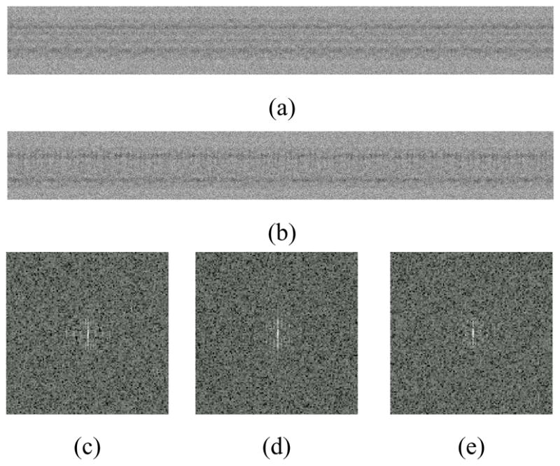
Real-space synthetic images of helices constructed from the ion channel pore. Both panels use the same intensity scale. Panel (a): Image of an object with Type 1 helical symmetry. Panel (b): Image of an object with Type 2 helical symmetry. Panels (c)–(e): Examples of log of squared magnitude of short images in reciprocal space.

Fig. 6.

Surface plots for the ion channel pore motif. Panels (a)–(c): True motif. Panels (d)–(f): 3-D reconstruction of the symmetric motif using 258 d_l,m,p coefficients. Panels (g)–(i): 3-D reconstruction of the motif without symmetry using 405 d_l,m,p coefficients. In the on-line version, the color map encodes distance from the origin in spherical coordinates.

Fig. 8.

FSC plots as functions of the magnitude of the reciprocal-space frequency vector k (Å⁻¹) for the ion channel pore example. Panel (a): The FSC curve is a comparison based on Eq. 38 of the reconstruction of the motif with the true motif used to make the synthetic images. Panel (b): The FSC curves are comparisons based on Eq. 39 of reconstructions of the helical objects with the true helical object used to make the synthetic images. Solid curve: 3-D reconstruction of Type 1 based on the symmetric motif using 258 d_l,m,p coefficients. Dotted curve: 3-D reconstruction of Type 2 based on the symmetric motif using 258 d_l,m,p coefficients. Dashed curve: 3-D reconstruction of Type 1 based on the motif without symmetry using 405 d_l,m,p coefficients. Dashed-dotted curve: 3-D reconstruction of Type 2 based on the motif without symmetry using 405 d_l,m,p coefficients.

Fig. 7.

Surface plots for the ion channel pore helical objects. Panels (a) and (b): True helical objects. Panels (c) and (d): 3-D reconstruction of the helical object based on the symmetric motif using 258 d_l,m,p coefficients. Panels (e) and (f): 3-D reconstruction of the helical object based on the motif without symmetry using 405 d_l,m,p coefficients. In the on-line version, the color map encodes distance from the z axis in cylindrical coordinates.

XI. Discussion and generalizations

Generalization of the methods described in this paper may be able to solve classification and 3-D reconstruction problems for objects with more complicated structure than an ideal helical symmetry. One type of problem is an object with essentially continuous variation in the parameters of the helical symmetry. If the parameters vary slowly along the axis of the helix then subdividing a long image into short images and treating each short image as described in this paper may be sufficient. However, if the variation is faster, then a stochastic process model for the local symmetry may be necessary. An advantage of the motif approach is that such a model might describe variations in z₀, φ₀, and r_H. These are more natural parameters for a physical model, because they describe assembly, than the u, v, and c parameters that are more often used to describe helical objects. A second type of problem is an object where even the motifs from the same class are heterogeneous. Such a problem might arise from true biological heterogeneity or be induced by sample preparation such as staining. By describing d_l,m,p coefficients as random variables with different pdfs for different classes, this type of problem has been successfully considered in a simpler context. In the standard Fourier-Bessel approach to describing helical objects, it is difficult to include such heterogeneity because the entire infinitely long helical object is described by a single set of coefficients and basis functions. Finally, both of these types of disorder might be simultaneously present, though the solution of such complicated problems would likely require extensive high quality image data.

Appendix A Class labels

The motif or the helical symmetry can change. The changes can be from one long image to another or within one long image. In the later case, we assume that each short image has constant motif and symmetry. A broad range of changes can be organized into the following seven cases. (1) All long images (or, equivalently, all short images) show objects sharing the same motif and symmetry. (2) Each long image shows an object with a fixed motif and symmetry but different long images can differ in (2a) symmetry but not motif, (2b) both symmetry and motif, and (2c) motif but not symmetry. (3) Each short image shows an object with a fixed motif and symmetry but different short images can differ in (3a) symmetry but not motif, (3b) both symmetry and motif, and (3c) motif but not symmetry.

Cases 2 and 3 of the previous paragraph imply that there is a label for either the long images (Case 2) or the short images (Case 3). If there is only one d but many (u, v) (Cases 2a and 3a), then the label is a label for (u, v). If there is only one (u, v) but many d (Cases 2c and 3c), then the label is a label for d. If there are many (u, v) and many d (Cases 2b and 3b), then the label is for triples (u, v, d). The first two cases are treated as special cases of the third, as is explained before Eq. 29 in Section VI. The work of this paper could be generalized to the case where there are two labels, one for (u, v) and one for d. In such a generalization, if there were two possible (u, v) and two possible d and an image could have any (u, v) paired with any d, then the algorithm would only estimate two (u, v) and two d rather than four (u, v) and four d as occurs when a single label labels triples (u, v, d). However, we are not aware of biological problems that need the level of generality achieved by two labels and so we have not pursued that case.

Appendix B Class labels: Classes α and β versus Classes 1, 2, and 3

The distinction between allowing motif or symmetry to change within one long image versus requiring both motif and symmetry to be constant within one long image but potentially change between long images is controlled by changing the indexed image to be the short image (N_s(i) = 1, Case 3 in Section IV and Appendix A) versus the long image (N_s(i) > 1, Case 2 in Section IV and Appendix A). Therefore both of these cases can be computed with the same equations. Cases α and β combined with the two N_s(i) situations described in this paragraph give six of the seven items listed in Section IV and Appendix A. Specifically Case α does Cases 2b, 2c, 3b, 3c while Case β does Cases 2a and 3a. Case 1 listed in Section IV and Appendix A is the elementary case where there is only one class and therefore only one motif and one symmetry. This case can be computed by either set of formulas.

References

- 1.Lee S, Doerschuk PC, Johnson JE. Reciprocal space representation of helical objects and their projection images for helices constructed from motifs without spherical symmetry. Ultramicroscopy. 2009;109:253–263. doi: 10.1016/j.ultramic.2008.10.014. [DOI] [PMC free article] [PubMed] [Google Scholar]
- 2.Egelman EH. The iterative helical real space reconstruction method: Surmounting the problems posed by real polymers. J Struct Biol. 2007;157(1):83–94. doi: 10.1016/j.jsb.2006.05.015. [DOI] [PubMed] [Google Scholar]
- 3.Holmes KC, Popp D, Gebhard W, Kabsch W. Atomic model of the actin filament. Nature. 1990;347:44–49. doi: 10.1038/347044a0. [DOI] [PubMed] [Google Scholar]
- 4.Milligan RA, Whittaker M, Safer D. Molecular structure of F-actin and location of surface binding sites. Nature. 1990;348:217–221. doi: 10.1038/348217a0. [DOI] [PubMed] [Google Scholar]
- 5.Li H, DeRosier DJ, Nicholson WV, Nogales E, Downing KH. Microtubule structure at 8Å resolution. Structure. 2002;10(10):1317–1328. doi: 10.1016/s0969-2126(02)00827-4. [DOI] [PubMed] [Google Scholar]
- 6.Yonekura K, Maki-Yonekura S, Namba K. Complete atomic model of the bacterial flagellar filament by electron cryomicroscopy. Nature. 2003;424:643–650. doi: 10.1038/nature01830. [DOI] [PubMed] [Google Scholar]
- 7.Yonekura K, Stokes DL, Sasabe H, Toyoshima C. The ATP-binding site of Ca2+-ATPase revealed by electron image analysis. Biophysical Journal. 1997;72(3):997–1005. doi: 10.1016/S0006-3495(97)78752-6. [DOI] [PMC free article] [PubMed] [Google Scholar]
- 8.Miyazawa A, Fujiyoshi Y, Unwin N. Structure and gating mechanism of the acetylcholine receptor pore. Nature. 2003;423:949–955. doi: 10.1038/nature01748. [DOI] [PubMed] [Google Scholar]
- 9.Wilson-Kubalek EM, Brown RE, Celia H, Milligan RA. Lipid nanotubes as substrates for helical crystallization of macromolecules. Proc Nat Acad Sci USA. 1998 July 7;95(14):8040–8045. doi: 10.1073/pnas.95.14.8040. [DOI] [PMC free article] [PubMed] [Google Scholar]
- 10.Dang TX, Farah SJ, Gast A, Robertson C, Carragher B, Egelman E, Wilson-Kubalek EM. Helical crystallization on lipid nanotubes: streptavidin as a model protein. J Struct Biol. 2005;150(2):90–99. doi: 10.1016/j.jsb.2005.02.002. [DOI] [PubMed] [Google Scholar]
- 11.Dang TX, Milligan RA, Tweten RK, Wilson-Kubalek EM. Helical crystallization on nickel-lipid nanotubes: Perfringolysin O as a model protein. J Struct Biol. 2005;152(2):129–139. doi: 10.1016/j.jsb.2005.07.010. [DOI] [PubMed] [Google Scholar]
- 12.Melia TJ, Sowa ME, Schutze L, Wensel TG. Formation of helical protein assemblies of IgG and transducin on varied lipid tubules. J Struct Biol. 1999;128(1):119–130. doi: 10.1006/jsbi.1999.4151. [DOI] [PubMed] [Google Scholar]
- 13.Egelman EH. A robust algorithm for the reconstruction of helical filaments using single-particle methods. Ultramicroscopy. 2000;85(4):225–234. doi: 10.1016/s0304-3991(00)00062-0. [DOI] [PubMed] [Google Scholar]
- 14.Carragher B, Whittaker M, Milligan RA. Helical processing using PHOELIX. J Struct Biol. 1996;116(1):107–112. doi: 10.1006/jsbi.1996.0018. [DOI] [PubMed] [Google Scholar]
- 15.Metlagel Z, Kikkawa YS, Kikkawa M. Ruby-Helix: an implementation of helical image processing based on object-oriented scripting language. J Struct Biol. 2007;157(1):95–105. doi: 10.1016/j.jsb.2006.07.015. [DOI] [PubMed] [Google Scholar]
- 16.Owen CH, Morgan DG, DeRosier DJ. Image analysis of helical objects: The Brandeis helical package. J Struct Biol. 1996;116(1):167–175. doi: 10.1006/jsbi.1996.0027. [DOI] [PubMed] [Google Scholar]
- 17.Crowther RA, Henderson R, Smith JM. MRC image processing programs. J Struct Biol. 1996;116(1):9–16. doi: 10.1006/jsbi.1996.0003. [DOI] [PubMed] [Google Scholar]
- 18.Frank J, Radermacher M, Penczek P, Zhu J, Li Y, Ladjadj M, Leith A. SPIDER and WEB: Processing and visualization of images in 3D electron microscopy and related fields. J Struct Biol. 1996;116:190–199. doi: 10.1006/jsbi.1996.0030. [DOI] [PubMed] [Google Scholar]
- 19.Cochran W, Crick FHC, Vand V. The structure of synthetic polypeptides. I. The transform of atoms on a helix. Acta Cryst. 1952;5:581–586. [Google Scholar]
- 20.Parent KN, Suhanovsky MM, Teschke CM. Polyhead formation in phage P22 pinpoints a region in coat protein required for conformational switching. Molecular Microbiology. 2007;65(5):1300–1310. doi: 10.1111/j.1365-2958.2007.05868.x. [DOI] [PMC free article] [PubMed] [Google Scholar]
- 21.Eads JL, Millane RP. Diffraction by the ideal paracrystal. Acta Crystallographica Section A. 2001 Sep;57(5):507–517. doi: 10.1107/s0108767301006341. [DOI] [PubMed] [Google Scholar]
- 22.Zheng Y, Doerschuk PC. A parallel software toolkit for statistical 3-D virus reconstructions from cryo electron microscopy images using computer clusters with multi-core shared-memory nodes. 22nd IEEE International Parallel and Distributed Processing Symposium (IPDPS 2008); April 14–18 2008; Miami, Florida: IEEE; pp. 1–11. [DOI] [Google Scholar]
- 23.Fernandez JJ, Sorzano COS, Marabini R, Carazo JM. Image processing and 3-D reconstruction in electron microscopy. IEEE Sig Proc Mag. 2006 May;23(3):84–94. [Google Scholar]
- 24.Yu Z, Bajaj C. Automatic ultrastructure segmentation of reconstructed CryoEM maps of icosahedral viruses. IEEE Trans Image Proc. 2005 Sep;14(9):1324–1337. doi: 10.1109/tip.2005.852770. [DOI] [PubMed] [Google Scholar]
- 25.Sorzano COS, Jonić S, El-Bez C, Carazo JM, De Carlo S, Thévenza P, Unser M. A multiresolution approach to orientation assignment in 3D electron microscopy of single particles. J Struct Biol. 2004;146(3):381–392. doi: 10.1016/j.jsb.2004.01.006. [DOI] [PubMed] [Google Scholar]
- 26.Marinescu DC, Ji Y. A computational framework for the 3D structure determination of viruses with unknown symmetry. J Parallel Distrib Comput. 2003;63(7/8):738–758. [Google Scholar]
- 27.Yin Z, Zheng Y, Doerschuk PC, Natarajan P, Johnson JE. A statistical approach to computer processing of cryo electron microscope images: Virion classification and 3-D reconstruction. J Struct Biol. 2003;144(1/2):24–50. doi: 10.1016/j.jsb.2003.09.023. [DOI] [PubMed] [Google Scholar]
- 28.Yin Z, Zheng Y, Doerschuk PC. An ab initio algorithm for low-resolution 3-D reconstructions from cryo electron microscopy images. J Struct Biol. 2001 Feb/Mar;133(2/3):132–142. doi: 10.1006/jsbi.2001.4356. [DOI] [PubMed] [Google Scholar]
- 29.Basu S, Bresler Y. Feasibility of tomography with unknown view angles. IEEE Trans Image Proc. 2000 Jun;9(6):1107–1122. doi: 10.1109/83.846252. [DOI] [PubMed] [Google Scholar]
- 30.Doerschuk PC, Johnson JE. Ab initio reconstruction and experimental design for cryo electron microscopy. IEEE Trans Info Theory. 2000 Aug;46(5):1714–1729. doi: 10.1109/18.857786. [DOI] [Google Scholar]
- 31.Erickson HP. The Fourier transform of an electron micrograph—First order and second order theory of image formation. In: Barer R, Cosslett VE, editors. Advances in Optical and Electron Microscopy. Vol. 5. London and New York: Academic Press; 1973. pp. 163–199. [Google Scholar]
- 32.Scherzer O. The theoretical resolution limit of the electron microscope. J Appl Phys. 1949 Jan;20:20–29. [Google Scholar]
- 33.Frank J. Three-Dimensional Electron Microscopy of Macromolecular Assemblies. San Diego: Academic Press; 1996. [Google Scholar]
- 34.Baker TS, Olson NH, Fuller SD. Adding the third dimension to virus life cycles: Three-dimensional reconstruction of icosahedral viruses from cryoelectron micrographs. Microbiology and Molecular Biology Reviews. 1999 Dec;63(4):862–922. doi: 10.1128/mmbr.63.4.862-922.1999. [DOI] [PMC free article] [PubMed] [Google Scholar]
- 35.Lee S. PhD dissertation. School of Electrical and Computer Engineering, Purdue University; West Lafayette, Indiana, USA: Aug, 2009. Maximum likelihood reconstruction of 3-D objects with helical symmetry from 2-D projections of unknown orientation and application to electron microscope images of viruses. [Google Scholar]
- 36.Moody MF. Image analysis of electron micrographs. In: Hawkes PW, Valdrè U, editors. Biophysical Electron Microscopy: Basic Concepts and Modern Techniques. ch 7. Academic Press; 1990. pp. 145–287. [Google Scholar]
- 37.Toyoshima C. Structure determination of tubular crystals of membrane proteins. I. Indexing of diffraction patterns. Ultramicroscopy. 2000;84(1/2):1–14. doi: 10.1016/s0304-3991(00)00010-3. [DOI] [PubMed] [Google Scholar]
- 38.Egelman EH. An algorithm for straightening images of curved filamentous structures. Ultramicroscopy. 1986;19(4):367–373. doi: 10.1016/0304-3991(86)90096-3. [DOI] [PubMed] [Google Scholar]
- 39.Lee J. PhD dissertation. School of Electrical and Computer Engineering, Purdue University; West Lafayette, Indiana, USA: Dec, 2006. A fast algorithm for maximum likelihood 3-D signal reconstruction from 2-D projections of unknown orientation and applications to the electron microscopy of viruses. [Google Scholar]
- 40.Dempster AP, Laird NM, Rubin DB. Maximum likelihood from incomplete data via the EM algorithm (with discussion) J Royal Stat Soc B. 1977;39:1–38. [Google Scholar]
- 41.Harauz G, van Heel M. Exact filters for general geometry three dimensional reconstruction. Optik. 1986;73(4):146–156. [Google Scholar]
- 42.Böttcher B, Wynne SA, Crowther RA. Determination of the fold of the core protein of hepatitis B virus by electron cryomicroscopy. Nature. 1997 March 6;386(6620):88–91. doi: 10.1038/386088a0. [DOI] [PubMed] [Google Scholar]
- 43.Namba K, Pattanayek R, Stubbs G. Visualization of protein-nucleic acid interactions in a virus: Refined structure of intact Tobacco Mosaic Virus at 2.9Å resolution by X-ray fiber diffraction. J Mol Biol. 1989;208(2):307–325. doi: 10.1016/0022-2836(89)90391-4. [DOI] [PubMed] [Google Scholar]
- 44.Jeng T-W, Crowther R, Stubbs G, Chiu W. Visualization of alpha-helices in Tobacco Mosaic Virus by cryoelectron microscopy. J Mol Biol. 1989;205:251–257. doi: 10.1016/0022-2836(89)90379-3. [DOI] [PubMed] [Google Scholar]
- 45.Zhu Y, Carragher B, Kriegman DJ, MRA, Potter CS. Automated identification of filaments in cryoelectron microscopy images. J Struct Biol. 2001;135(3):302–312. doi: 10.1006/jsbi.2001.4415. [DOI] [PubMed] [Google Scholar]
- 46.Carragher B, Fellmann D, Guerra F, Milligan RA, Mouche F, Pulokas J, Sheehan B, Quispe J, Suloway C, Potter CS. Rapid, routine structure determination of macromolecular assemblies using electron microscopy: current progress and further challenges. J Synchrotron Rad. 2004;11:83–85. doi: 10.1107/s0909049503023987. [DOI] [PubMed] [Google Scholar]
- 47.Sachse C, Chen JZ, Coureux P-D, Stroupe ME, Fändrich M, Grigorieff N. High-resolution electron microscopy of helical specimens: A fresh look at Tobacco Mosaic Virus. J Mol Biol. 2007 Aug 17;371:812–835. doi: 10.1016/j.jmb.2007.05.088. [DOI] [PMC free article] [PubMed] [Google Scholar]
- 48.Pettersen EF, Goddard TD, Huang CC, Couch GS, Greenblatt DM, Meng EC, Ferrin TE. UCSF Chimera—A visualization system for exploratory research and analysis. J Comput Chem. 2004;25(13):1605–1612. doi: 10.1002/jcc.20084. [DOI] [PubMed] [Google Scholar]
- 49.Alam A, Jiang Y. High-resolution structure of the open NaK channel. Nature Structural and Molecular Biology. 2009 Jan;16(1):30–34. doi: 10.1038/nsmb.1531. [DOI] [PMC free article] [PubMed] [Google Scholar]