Estimation in Medical Imaging without a Gold Standard

Abstract

Rationale and Objectives

In medical imaging, physicians often estimate a parameter of interest (eg, cardiac ejection fraction) for a patient to assist in establishing a diagnosis. Many different estimation methods may exist, but rarely can one be considered a gold standard. Therefore, evaluation and comparison of different estimation methods are difficult. The purpose of this study was to examine a method of evaluating different estimation methods without use of a gold standard.

Materials and Methods

This method is equivalent to fitting regression lines without the x axis. To use this method, multiple estimates of the clinical parameter of interest for each patient of a given population were needed. The authors assumed the statistical distribution for the true values of the clinical parameter of interest was a member of a given family of parameterized distributions. Furthermore, they assumed a statistical model relating the clinical parameter to the estimates of its value. Using these assumptions and observed data, they estimated the model parameters and the parameters characterizing the distribution of the clinical parameter.

Results

The authors applied the method to simulated cardiac ejection fraction data with varying numbers of patients, numbers of modalities, and levels of noise. They also tested the method on both linear and nonlinear models and characterized the performance of this method compared to that of conventional regression analysis by using x-axis information. Results indicate that the method follows trends similar to that of conventional regression analysis as patients and noise vary, although conventional regression analysis outperforms the method presented because it uses the gold standard which the authors assume is unavailable.

Conclusion

The method accurately estimates model parameters. These estimates can be used to rank the systems for a given estimation task.

Much of the recent research in medical imaging has dealt with the development of imaging systems or of image-processing techniques to produce “better” images. Thus, regardless of the imaging modality involved, a definition of what constitutes a “better” image is required. One common approach to the assessment of image quality is visual comparison by human observers. This method, however, is both subjective and often irreproducible. A more scientific and objective approach to assessing image quality is one based on task performance (1). To implement this approach, three elements much be specified: (a) the task for which the images are being produced, (b) the observer who will perform this task, and (c) the patient population being imaged. Typical tasks are the detection of an abnormality, the estimation of some parameter of interest, or some combination thereof. A given imaging system may be more suited for certain tasks, thereby requiring a clear definition of the task itself to assess objective image quality. The observer is usually a human, but it can also be a computer program (or some combination of the two). The patient population is the group of subjects to be imaged. For example, if imaging is being performed to detect liver tumors, then the patient population consists of those patients who are at risk for liver cancer.

Conventionally, we employ a gold standard to measure the performance of an observer by using a particular imaging system for detection or estimation. A gold standard is a method that is presumed to be correct for determining the presence of an abnormality or the parameter being estimated. For example, for the detection of breast tumors on screening mammograms, the gold standard is the examination of surgically obtained specimens by a pathologist (2). Because of the invasive nature of most gold standards, the ability to measure task performance without use of a gold standard is of considerable interest to the imaging community (3).

In the case of detection tasks, common measurements of performance are various features of the receiver operating characteristic (ROC) curve (4). This type of analysis required a gold standard until Henkelman et al (5) developed a technique to compute ROC curves for multiple imaging modalities without use of a gold standard.

For performance measurements involving an estimation task and a gold standard, we can plot the estimate versus the gold standard for each patient and then use statistical techniques (eg, linear regression) to determine the relationship between them. Estimation methods with small bias and little noise are preferable.

The purpose of this study was to examine a method of evaluating different estimation methods without use of a gold standard. This amounts to performing “regression without the truth” (ie, the x axis), from which the title of this technique (RWT) is derived.

MATERIALS AND METHODS

A variety of different parameters are estimated in medical imaging in an attempt to quantify an individual’s health status. For example, the cardiac ejection fraction describes the fraction of the blood in the left ventricle that is pumped out during a given cycle. This parameter, which is used by physicians as an indicator of a patient’s susceptibility to heart failure, can be estimated with use of ultrasound (US), magnetic resonance (MR), or gamma-ray imaging techniques (6,7). When evaluating a new method to estimate the cardiac ejection fraction, it is common practice to use a more accepted modality as a pseudo– gold standard. There is no a priori reason, however, to believe that any of these techniques provides the true value of the parameter of interest. Many other quantities that are estimated in medical imaging also lack a gold standard; examples include the blood oxygen concentration (8) and bone density (9).

In this study, we assumed that a true value exists for the cardiac ejection fraction in each patient, but that this value is unknown to us. Let us envision an experiment estimating a clinically relevant parameter for P patients using M different modalities. We denote the estimated parameter for the pth patient and mth modality by θ_pm and the true value (ie, the unknown gold standard) for the pth patient by Θ_p. We assume that these quantities are related by

$${\mathit{\theta }}_{\mathit{\text{pm}}}=a_m{\mathbf{\Theta }}_p+b_m+{\mathit{\epsilon }}_{\mathit{\text{pm}}},$$ (1)

where a_m and b_m are the linear model parameters and ε_pm is the random noise in the measurement. We also assume for a given modality m that ε_pm follows a normal distribution with a mean of zero and a standard deviation of σ_m; that is, for a given patient p,

$$\mathit{\text{pr}}(\{{\mathit{\epsilon }}_{\mathit{\text{pm}}}\})={\displaystyle \prod _{m=1}^M}\frac{1}{\sqrt{2\pi {\mathit{\sigma }}_m^2}}\text{exp}\left(-\frac{1}{2{\mathit{\sigma }}_m^2}{\mathit{\epsilon }}_{\mathit{\text{pm}}}^2\right),$$ (2)

where pr({ε_pm}) denotes pr(ε_p1, ε_p2, …, ε_pM). In formulating Equation (2), we assume that the noise is independent across modalities and patients (ie, the noise in MR imaging is independent of the noise in ultrasound), and that the cardiacl ejection fraction of one patient does not affect that of another. Using Equation (1), we arrive at

$$\mathit{\text{pr}}(\{{\mathit{\theta }}_{\mathit{\text{pm}}}\}|\{a_m,b_m,{\mathit{\sigma }}_m\},{\mathbf{\Theta }}_p)={\displaystyle \prod _{m=1}^M}\frac{1}{\sqrt{2\pi {\mathit{\sigma }}_m^2}}\text{exp}\left(-\frac{1}{2{\mathit{\sigma }}_m^2}{[{\mathit{\theta }}_{\mathit{\text{pm}}}-a_m{\mathbf{\Theta }}_p-b_m]}^2\right).$$ (3)

Note that the terms a_m, b_m, and σ_m, which make up the linear model describing each modality, depend only on the modality; they are independent of the patient. Although a linear model is assumed here, the RWT method is also applicable to nonlinear models (discussed later).

In addition, we assume the gold standard for each patient, Θ_p, is the same for each modality. Furthermore, we assume that a probability distribution exists on Θ, pr(Θ), from which the Θ_p values are drawn as independent samples. Using a probabilistic view of Θ enables us to compute the likelihood, L(·), that we observed our data given the model parameters. This is accomplished by marginalizing over the variable Θ_p,

$$L(\{a_m,b_m,{\mathit{\sigma }}_m\}|D)={\displaystyle \prod _{p=1}^P}\mathit{\text{pr}}(\{{\mathit{\theta }}_{\mathit{\text{pm}}}\}|\{a_m,b_m,{\mathit{\sigma }}_m\})={\displaystyle \prod _{p=1}^P}{\displaystyle \int }\mathit{\text{pr}}(\{{\mathit{\theta }}_{\mathit{\text{pm}}}\}|\{a_m,b_m,{\mathit{\sigma }}_m\},\mathbf{\Theta })\mathit{\text{pr}}(\mathbf{\Theta })d\mathbf{\Theta },$$ (4)

where pr({θ_pm}|{a_m, b_m, σ_m}, Θ) is given in Equation (3) and D is the data θ_pm for all observed patients and modalities. If we knew the density function pr(Θ), we would use it to calculate this likelihood. We do not know this density function, however. Thus, we represent pr(Θ) by parameterized density function $\widehat{\mathit{\text{pr}}}(\mathbf{\Theta }|\overrightarrow{r})$, where the components of r⃗ are parameters that we can vary. For example, in the case of a normal distribution, we would vary the mean and that standard deviation; thus, we have a likelihood that is a function both of the linear model parameters and of the gold-standard density parameters. Our goal is to use data from P patients for whom the parameter of interest has been estimated on M > 1 modalities to determine estimates for a_m, b_m, σ_m, and r⃗ (denoted by â_m, b̂_m, σ̂_m, and r⃗̂, respectively) by maximizing the expression for the likelihood of the data. This estimation method is commonly referred to as maximum-likelihood (ML) estimation (10). The parameter values determined with ML estimation characterize the relationship between the estimates and the gold standard of each modality, the noise in these estimates, and the distribution of the true values for the patient population. A detailed derivation has been published previously (11).

Many other methods are available for estimating these values, but ML estimation has the advantage of being relatively easy to implement and of being asymptotically efficient. An efficient estimator is one that is unbiased (ie, yielding the correct value on average) and that has minimum variance in the class of all such unbiased estimators (12). By “asymptotically efficient,” we mean that the ML estimator tends to an efficient estimator as the patient population increases. Note that estimation of the parameters a_m, b_m, σ_m, and r⃗ is guaranteed to be asymptotically efficient only when the linear model is correct and the parameterized density is capable of matching the true density of the gold standard.

Implementation

The likelihood function was implemented and optimized on an 800-MHz Pentium III computer (Dell, Round Rock, Tex) by using Matlab software (Mathworks, Natick, Mass). We used a quasi-Newton optimization method in the Matlab software to determine the maximum of the likelihood. We constrained this optimization to look for reasonable values of the parameters (ie, positive slopes and positive variances). We fixed the initial guess as the midpoint of the search space, which was a point not equal to the true values of the parameters. Using these constraints, the results of the optimization were not sensitive to the initial guess. The optimization task itself took from a few seconds to a few minutes to run, depending on the form of the assumed distribution that was used in the likelihood expression.

We performed numerous simulation studies in which we sampled cardiac ejection fractions (ie, the gold standard) for a simulated patient population from a beta distribution with fixed parameters; that is, pr(Θ) was beta distributed. We then adjusted this gold standard by using linear models with known parameters a_m and b_m and a known noise level characterized by σ_m. This comprised the data that were input for the RWT; the gold standard values were not input for the RWT. In computing the likelihood function, we not only need the data but must also assume a functional form for the gold-standard density. Thus, we assumed a truncated normal distribution with a varying mean and variance; that is, p(Θ|r⃗) was a truncated normal density with r⃗ = {μ_a,σ_a}. Note that this distribution differs from what was actually used to generate the gold standard. This simulates the real-world situation in which one would not know exactly how the gold standard was distributed.

Both the beta and the truncated normal distributions are bounded between zero and one. This study examined the performance of RWT only with these bound distributions. (Difficulties that arise when extending the RWT method to distributions spanning the entire real line will be the subject of future work.) Both of the distributions employed are unimodal (ie, single peaked). One might expect the distribution of cardiac ejection fractions to be bimodal, with one peak for the patients with heart problems and one peak for the patients without heart problems, but Sharir et al (7) have presented data to support a unimodal model for the distribution of cardiac ejection fractions.

Illustrative Example

An illustrative example may help explain the RWT method further. For the numeric simulations throughout this study, we generate Θ_p values (ie, the gold standard) by sampling a known distribution. From this, we can generate the estimates for each modality (ie, the θ_pm values) by using Equation (1). We use RWT to estimate the linear model parameters a_m, b_m, and σ_m and the parameters that determine the shape of pr(Θ) by using only the θ_pm values. This is accomplished by maximizing a likelihood expression with numeric optimization techniques.

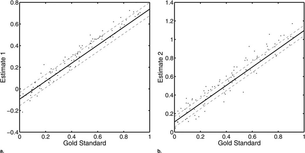
Figure 1 displays a plot of θ_pm versus Θ_p for M = 2 modalities and P = 100 patients. Also plotted are the regression lines derived using the estimated linear model parameters. We stress that the gold standard was not used in the estimation of these linear model parameters. Thus, one could think of this figure as being a linear-regression analysis that was performed without knowledge of the x-coordinates.

Figure 1.

A graphic, two-modality example of the method studied where a shows the results for M = 1 and b shows the results for M = 2. The dotted lines represent ±σ̂_m. The slope, intercept, and noise terms were estimated by using RWT. Although the x coordinates are plotted, they were not used in estimating the linear model parameters.

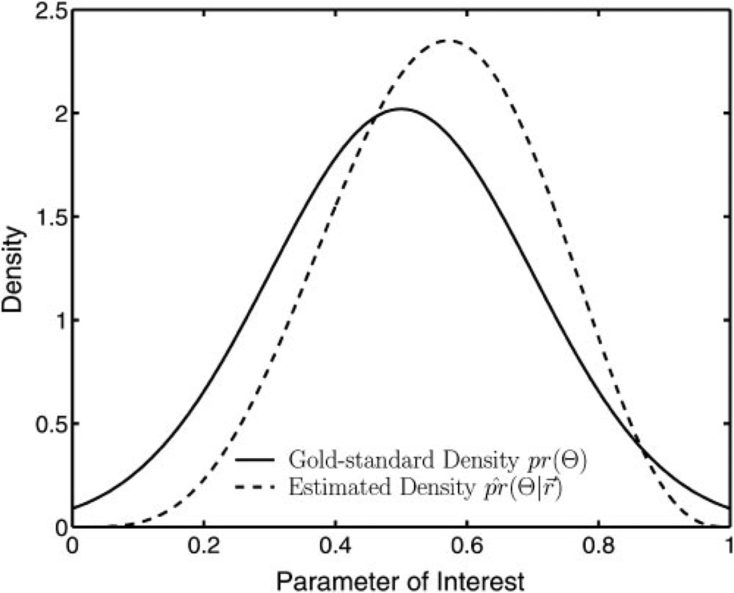
Figure 2 displays a plot of the density associated with the gold standard, pr(Θ), along with the density $\widehat{\mathit{\text{pr}}}(\mathbf{\Theta }|\widehat{\overrightarrow{r}})$ by using r⃗ as determined with RWT. In this example, the gold standard was sampled from a truncated normal distribution. A beta distribution with two varying parameters, r⃗, was used as the assumed distribution. This is the opposite of what was done in the later simulation studies, in which the gold standard was a beta distribution and the model employed was a truncated normal distribution. With certain choices regarding the parameters, the beta distribution can look very different from a normal distribution. However, the distribution parameters fit by RWT, r⃗̂, are such that the beta distribution looks similar to that of the truncated normal distribution that was used to generate the gold standard.

Figure 2.

A comparison of the true gold-standard density, pr(Θ), and the parameterized density, $\widehat{\mathit{\text{pr}}}(\mathbf{\Theta }|\widehat{\overrightarrow{r}})$. The shape of the density, as characterized by r⃗, was determined with RWT but without previous information. The gold-standard density shown here is a truncated normal density, whereas the parameterized density used in the likelihood expression is a beta-density function. In a sense, this illustrates a beta density imitating a given truncated normal density. Note that the parameter of interest is limited to a finite domain.

Figure of Merit

The figure of merit in linear-regression analysis is the root-mean-squared error (RMSE), hence the expression least-squares fitting. We use a similar figure of merit to characterize the performance of a single application of RWT. The RMSE for a given modality m is

$${\text{RMSE}}_m=\sqrt{\frac{1}{P}{\displaystyle \sum _{p=1}^P}{\left({\mathbf{\Theta }}_p-\frac{{\mathit{\theta }}_{\mathit{\text{pm}}}-{\widehat{b}}_m}{{\widehat{a}}_m}\right)}^2}.$$ (5)

This figure of merit was chosen because it measures the difference between the gold standard, Θ_p, and the values found through adjusting the data, θ_pm, by the estimated linear model parameters, â_m and b̂_m. Note that this figure of merit cannot be used in practice, however, because of the lack of a gold standard, but it provides an excellent technique to evaluate the method in a simulation. In this study, we performed 50 simulations and average RMSE_m determinations (denoted by RMSE_m) and also computed the standard error.

RESULTS

Analysis of RWT

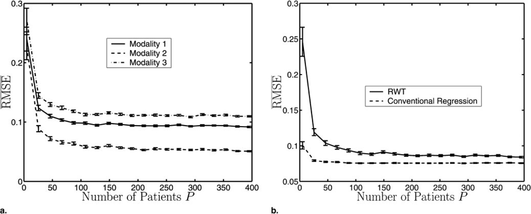
As stated, ML estimation is asymptotically efficient. Figure 3a shows that the $\overline{\text{RMSE}}$, as given in Equation (5), decreases as the patient number increases. The variance of the noise σ_m was fixed for each modality in this experiment. In the limit of large patient numbers, the three different curves (each representing a different modality) tend to a minimum value σ_m/a_m (see Eqq [1] and [5]) in accordance with ML theory.

Figure 3.

(a) The $\overline{\text{RMSE}}$ for three different modalities versus the number of patients. As the number of patients increases, RMSE_m converges to σ_m/a_m by Equations (1) and (5). (b) A comparison between RWT and linear-regression analysis with a gold standard. Note that the RMSE is also averaged over the three modalities. As expected, conventional regression analysis has lower RMSE, but the performances of the two methods converge as the number of patients increases. For these experiments, a⃗ = [0.6,0.7,0.8], b⃗ = [−0.1,0.0,0.1], σ⃗ = [0.05,0.03,0.08], and the error bars represent the standard error calculated over 50 independent experiments.

Figure 3b compares the performance of conventional regression analysis with that of RWT. As expected, conventional regression analysis using the gold standard outperforms RWT. The difference between the two, however, decreases as a function of the size of the patient population.

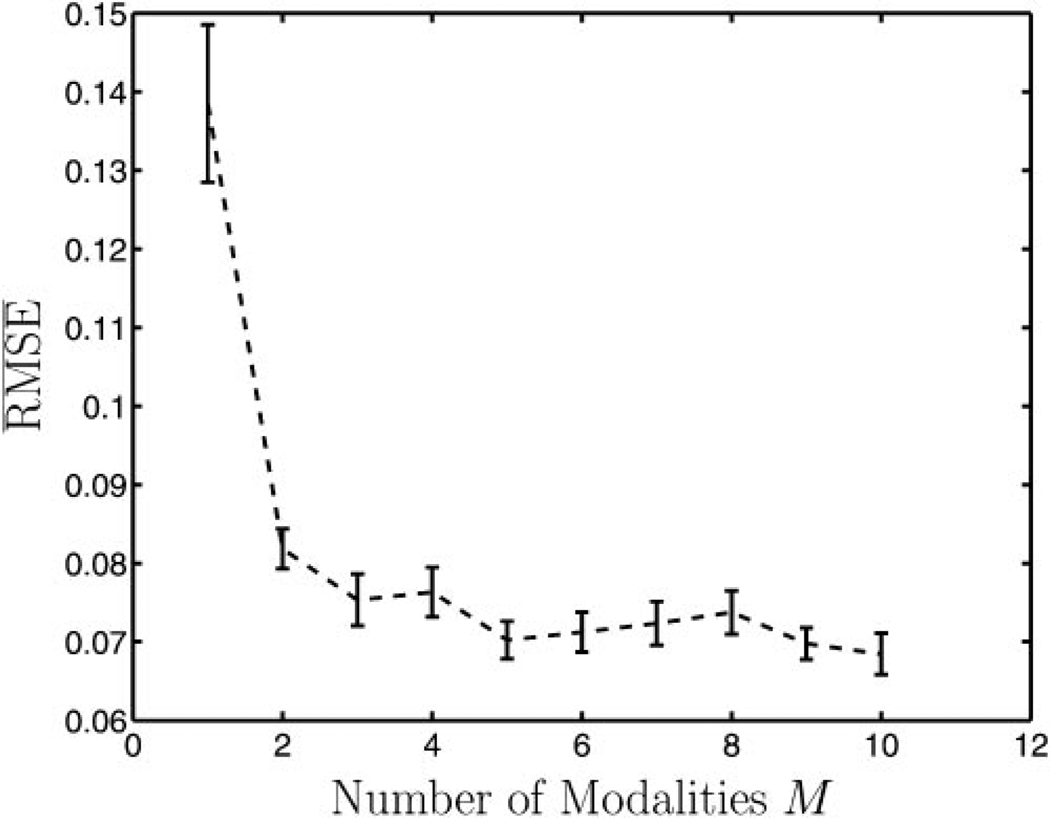
That an increase in data yields more accurate results is not surprising. An increase in the number of modalities, however, is a somewhat less intuitive notion given the complexity of our ML estimator. Figure 4 displays a plot of $\overline{\text{RMSE}}$ versus number of modalities. After a few modalities, the gain in accuracy is not substantial. Note that the performance of conventional linear-regression analysis is independent of the number of modalities. The performance of RWT with one modality is very poor, but the performance with two or more modalities is relatively constant.

Figure 4.

The $\overline{\text{RMSE}}$ (averaged across simulations and modalities) versus the number of modalities used in a RWT experiment. A sharp decline in $\overline{\text{RMSE}}$ is seen from one to two modalities, followed by a slow decline. One might expect this, especially because RWT cannot work properly with only one modality. The performance of conventional regression analysis is independent of the number of modalities. The same model parameters were used for all modalities in all experiments (a_m = 1, b_m = 0.1, σ_m = 0.05, P = 100).

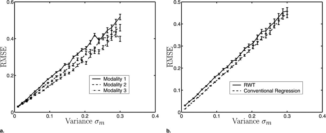
Finally, we looked at the impact on $\overline{\text{RMSE}}$ of varying the parameter σ_m to understand what occurs regarding accuracy as the noise in the data increases. The curves in Figure 5a show that $\overline{\text{RMSE}}$ increases linearly with increases in σ_m. The slopes of these lines are given by 1/a_m, as predicted from Equations (1) and (5).

Figure 5.

(a) The $\overline{\text{RMSE}}$ for three different modalities versus variance of the noise σ_m. The $\overline{\text{RMSE}}$ increases in accordance with 1/a_m by Equations (1) and (5). (b) A comparison between RWT and linear-regression analysis with a gold standard. Note that the RMSE is also averaged over the three modalities. The $\overline{\text{RMSE}}$ does not converge to zero for RWT as σ_m tends to zero. The parallel nature of the two graphs indicates that the comparative performance of RWT is independent of σ_m. For these experiments, a⃗ = [0.6,0.7,0.8], b⃗ = [−0.1,0.0,0.1], P = 100, and the error bars represent the standard error calculated over 50 independent experiments.

Figure 5b compares the performance of conventional regression analysis with that of RWT. Whereas the $\overline{\text{RMSE}}$ limits to zero as σ_m → 0 for conventional regression analysis, RWT limits to a positive constant. The constant difference between the two plots in Figure 5b indicates the independent relationship between the variance of the noise and the comparative performance of RWT and conventional regression analysis.

Nonlinear Models

A clear limitation of the results presented thus far is the strict assumption of a linear model governing the relationship between the gold standard and the individual modalities. To ease this assumption, one can rewrite Equation (1) as

$${\mathit{\theta }}_{\mathit{\text{pm}}}=N({\mathbf{\Theta }}_p,{\overrightarrow{\mathit{\nu }}}_m)+{\mathit{\epsilon }}_{\mathit{\text{pm}}},$$ (6)

where N(·) is some nonlinear function of the gold standard with the model parameters ν⃗_m.

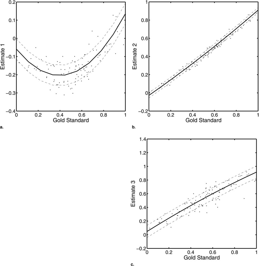
Figure 6 shows the results of a single experiment using a quadratic model for each of three modalities. With modality 1 (Fig 6a), a nonlinear relationship is seen between the gold standard and the estimate. With modality 2 (Fig 6b), a weak, nonlinear relationship is seen. Finally, the relationship in modality 3 (Fig 6c) is linear. The RWT accurately fits all three modalities. The time required for the optimization procedure to converge, however, is increased by the added parameters to be estimated. Also, with too many parameters, regression analysis will eventually fit the noise in the data. We have shown that the method can be extended to nonlinear models, but extensive work remains to be completed with the linear models before the performance of this technique using nonlinear models can be fully characterized.

Figure 6.

An application of RWT with a quadratic model. (a) For modality 1, a strong, nonlinear relationship with the gold standard and a relatively large variance were discovered qualitatively. (b) Modality 2 was slightly nonlinear with a small variance, whereas (c) modality 3 was linear with a large variance. Both were fit well by the quadratic RWT.

DISCUSSION

Arriving at a gold standard for a given estimation task is often difficult. Frequently, researchers in a given field do not agree on a gold standard, and even when such agreement occurs, the information can be difficult to obtain (eg, by means of postmortem examination). Indeed, if an accepted gold standard was easy to obtain, no other methods to ascertain the relevant information would be needed. Thus, a gold standard typically is not available.

In the absence of a gold standard, an alternate approach to comparing estimation tasks in medical imaging involves plotting the results obtained with a new modality versus those obtained with a more established modality. These results give us a pseudo– gold standard for a common patient population (13). Such comparisons are not necessarily meaningful, however, given the inaccuracy of the pseudo– gold standard. We have presented a method to compare and to evaluate different estimation techniques without use of a gold standard.

An estimator of a medically relevant parameter should be both accurate and precise. For the linear models discussed in this study, accuracy can be approximately achieved by adjusting the measurements using the estimated model parameters â_m and b̂_m. After this correction has been made, the variance in the adjusted measurements (ie, the precision) is ${\mathit{\sigma }}_m^2/{\widehat{a}}_m^2$. An estimate of this quantity ${\widehat{\mathit{\sigma }}}_m^2/{\widehat{a}}_m^2$ can be used as a figure of merit for cross-modality comparisons.

The key advantage of RWT over conventional regression analysis is that RWT does not require use of a gold standard. The performance of RWT is, however, hindered by this lack of information. Furthermore, like conventional regression analysis, RWT involves the assumption of a known functional form for the relationship between the gold standard and the data, but unlike the case with conventional regression analysis, this relationship cannot be visually assessed without the gold standard. We must also assume a functional form of the gold standard density, pr(Θ), but some or all parameters characterizing the shape of this density are free to vary in RWT. In this study, we have assumed a Gaussian noise model, which is also implicit in conventional regression analysis, but other noise models are easy to implement in the likelihood expression.

A principal weakness of RWT is the assumption that the gold standard for a particular patient Θ_p does not vary across modalities. For example, a patient’s heart rate and, hence, ejection fraction might vary if measured with MR imaging because of the enclosed nature of many MR imaging machines. Variations in the gold standard can be accounted for, to first order, by the modality noise term ε_pm if the variations in the gold standard are assumed to have a mean of zero and constant variance.

We have previously studied the bias and variance of estimated parameters in this technique when the true and assumed distributions differed (11). Reference 11 used only beta and truncated normal distributions, and we found that parameters were accurately estimated even when the distributions did not match. We are performing ongoing studies in which the shapes of the assumed and true distributions differ greatly. For example, with diseased and nondiseased patient populations, one might expect to see a bimodal distribution for the gold standard. We are currently using a parameterized, bimodal distribution in the likelihood expression. Furthermore, we are examining goodness-of-fit measures to determine how well the parameters characterizing the shape of the gold-standard density are estimated. Finally, we are studying the theoretic performance limit of RWT; that is, we have calculated the Fisher information matrix for this problem and used it to determine the minimum possible variances that an unbiased estimator can have for this problem. This type of analysis allows us to study and to quantify the limitations of the RWT technique.

Conventional regression analysis uses more information than RWT (ie, the x axis). A noteworthy aspect of RWT, however, is the exploitation of previously unused information. We have shown that we can successfully estimate model parameters without the x axis if we have measurements obtained from multiple modalities for a common group of patients.

REFERENCES

- 1.Barrett HH. Objective assessment of image quality: effects of quantum noise and object variability. J Opt Soc Am A. 1990;7:1266–1278. doi: 10.1364/josaa.7.001266. [DOI] [PubMed] [Google Scholar]
- 2.Feig SA. Estimation of currently attainable benefit from mammographic screening in women aged 40–49. Cancer. 1995;75:2412–2419. doi: 10.1002/1097-0142(19950515)75:10<2412::aid-cncr2820751005>3.0.co;2-4. [DOI] [PubMed] [Google Scholar]
- 3.Walter SD, Irwig LM. Estimation of test error rates, disease prevalence, and relative risk from misclassified data: a review. J Clin Epidemiol. 1988;41:923–937. doi: 10.1016/0895-4356(88)90110-2. [DOI] [PubMed] [Google Scholar]
- 4.Metz CE. ROC methodology in radiologic imaging. Invest Radiol. 1986;21:720–733. doi: 10.1097/00004424-198609000-00009. [DOI] [PubMed] [Google Scholar]
- 5.Henkelman RM, Kay I, Bronskill MJ. Receiver operator characteristic (ROC) analysis without truth. Med Decis Making. 1990;10:24–29. doi: 10.1177/0272989X9001000105. [DOI] [PubMed] [Google Scholar]
- 6.Rumbereger JA, Behrenbeck T, Bell MR, et al. Determination of ventricular ejection fraction: a comparison of available imaging methods. Mayo Clin Proc. 1997;72:860–870. doi: 10.4065/72.9.860. [DOI] [PubMed] [Google Scholar]
- 7.Sharir T, Germano G, Kang X, et al. Prediction of myocardial infarction versus cardiac death by gated myocardial perfusion SPECT: risk stratification by the amount of stress-induced ischemia and the poststress ejection fraction. J Nucl Med. 2001;42:831–837. [PubMed] [Google Scholar]
- 8.Al-Hallaq H, River JN, Zamora M, et al. Correlation of magnetic resonance and oxygen microelectrode measurements of carbogen-induced changes in tumor oxygenation. Int J Radiat Oncol Biol Phys. 1998;41:151–159. doi: 10.1016/s0360-3016(98)00038-8. [DOI] [PubMed] [Google Scholar]
- 9.Sturtridge W, Lentle B, Hanley DA. Prevention and management of osteoporosis: consensus statements from the scientific advisory board of the Osteoporosis Society of Canada. Can Med Assoc J. 1996;155:924–929. [PMC free article] [PubMed] [Google Scholar]
- 10.Van Trees HL. Detection, estimation, and modulation theory: part I. New York, NY: Wiley; 1968. [Google Scholar]
- 11.Hoppin J, Kupinski M, Kastis G, Clarkson E, Barrett HH. Objective comparison of quantitative imaging modalities without the use of a gold standard. In: Insana M, Leahy R, editors. Lecture notes in computer science: information processing in medical imaging. New York, NY: Springer; 2001. pp. 12–23. [Google Scholar]
- 12.Papoulis A. Probability, random variables, and stochastic processes. New York, NY: McGraw-Hill; 1991. [Google Scholar]
- 13.Cwajg E, Cwajg J, He ZX, et al. Gated myocardial perfusion tomography for the assessment of left ventricular function and volumes: comparison with echocardiography. J Nucl Med. 1999;40:1857–1865. [PubMed] [Google Scholar]