Optimizing reproductive phenology in a two-resource world: a dynamic allocation model of plant growth predicts later reproduction in phosphorus-limited plants

Abstract

Background and Aims

Timing of reproduction is a key life-history trait that is regulated by resource availability. Delayed reproduction in soils with low phosphorus availability is common among annuals, in contrast to the accelerated reproduction typical of other low-nutrient environments. It is hypothesized that this anomalous response arises from the high marginal value of additional allocation to root growth caused by the low mobility of phosphorus in soils.

Methods

To better understand the benefits and costs of such delayed reproduction, a two-resource dynamic allocation model of plant growth and reproduction is presented. The model incorporates growth, respiration, and carbon and phosphorus acquisition of both root and shoot tissue, and considers the reallocation of resources from senescent leaves. The model is parameterized with data from Arabidopsis and the optimal reproductive phenology is explored in a range of environments.

Key Results

The model predicts delayed reproduction in low-phosphorus environments. Reproductive timing in low-phosphorus environments is quite sensitive to phosphorus mobility, but is less sensitive to the temporal distribution of mortality risks. In low-phosphorus environments, the relative metabolic cost of roots was greater, and reproductive allocation reduced, compared with high-phosphorus conditions. The model suggests that delayed reproduction in response to low phosphorus availability may be reduced in plants adapted to environments where phosphorus mobility is greater.

Conclusions

Delayed reproduction in low-phosphorus soils can be a beneficial response allowing for increased acquisition and utilization of phosphorus. This finding has implications both for efforts to breed crops for low-phosphorus soils, and for efforts to understand how climate change may impact plant growth and productivity in low-phosphorus environments.

INTRODUCTION

The timing of reproduction is a key determinant of fitness (Stearns, 1992). Plants undergo a period of strictly vegetative growth prior to initiating reproductive activity, which permits the development of resource acquisition capacity and resource stores that can be utilized in reproductive growth. Earlier reproduction avoids the risk of mortality later in the growing season, but earlier reproduction carries an opportunity cost – resources not captured as a result of investment in reproduction rather than growth (Reekie and Bazzaz, 1987). Optimal timing of reproduction involves a trade-off between the benefit of delaying reproduction – increased resources acquired because of a longer period of somatic growth – and the risk of reduced reproductive success caused by the increased risk of mortality.

In general, the length of growing season would be expected to be correlated with greater yield potential (Manske et al., 2000; Beaver et al., 2003). The implications of this general trend for low-nutrient environments are unclear. Clearly, the dynamics of distinct nutrients may play a role. Phosphorus, potassium and ammonium are generally immobile, and their acquisition is limited by diffusion, while nitrate, sulphate, calcium and magnesium are soluble and are acquired with bulk flow of soil solution driven by transpiration (Barber, 1995). The effects of nutrient mobility on the response of plant growth to length of growing season are poorly understood, but probably important (Nord and Lynch, 2009). For common bean, Araujo et al. (1998) proposed that fast growth and earlier flowering may be favoured in resource-rich environments, while slow growth and late flowering would be preferable in resource-poor environments because slower growth rates allow more efficient reutilization of phosphorus, and later maturation allows a longer period for nitrogen fixation.

Plant growth and productivity are frequently limited by low phosphorus availability (Lynch and Deikman, 1998; Fairhurst et al., 1999). Phosphate has multiple reactions with soil constituents that reduce both its bioavailability (Comerford, 1998) and mobility in most soils (Barber, 1995). Phosphorus diffuses very slowly in soils, with diffusion coefficients of 10⁻⁷ to 10⁻⁹ cm² s⁻¹ (Schenk and Barber, 1979), but diffusion is the primary mode of phosphorus transport to roots. Mechanistic models estimate that over 90 % of phosphorus acquired by plants reaches the roots via diffusion (Barber, 1995). Phosphorus uptake via diffusion is maximized by increasing root exploration of virgin soil (which reduces the distance over which phosphorus must diffuse to reach a root), and by increasing time during which diffusion may occur. The reduction in vegetative (and hence root) growth that accompanies the transition to reproductive growth has the potential to limit phosphorus acquisition, and delaying reproduction might be disproportionately beneficial for phosphorus acquisition.

Annual plants in stressful conditions generally flower and mature earlier than plants in benign conditions (Pigliucci and Schlichting, 1995; Gungula et al., 2003; Callahan and Pigliucci, 2005). Several models of plant phenology predict this response (Cohen, 1976; Amir and Cohen, 1990). In contrast, low phosphorus availability typically delays plant phenology (Rossiter, 1978; Shepherd et al., 1987; Ma et al., 2002). Nord and Lynch (2008) showed that delayed phenology may be an adaptive response to low phosphorus availability in Arabidopsis thaliana, by allowing more time for phosphorus acquisition and utilization.

The degree to which nutrients in vegetative tissue can later be reallocated to reproduction is important in determining how nutrient allocation to vegetative growth affects subsequent reproduction. Nutrients are typically reallocated from leaves as part of the leaf senescence programme. Both nitrogen and phosphorus resorption from leaves can be highly efficient with reported values of up to 90 % (Aerts et al., 1992; Aerts, 1996; Aerts and Chapin, 2000). The high rates of reproductive tissue growth in annuals should mean that sink strength would be high, potentially increasing resorption efficiency. Just how this reallocation is affected by phosphorus availability is unclear. In one study with common bean, leaf phosphorus remobilization occurred earlier under phosphorus deficiency (Snapp and Lynch, 1996).

It appears that root nutrients are not reallocated, or are reallocated with very low efficiency. Aerts et al. (1992) and Gordon and Jackson (2000) report little or no resorption of root nutrients. Roots of common bean retain phosphorus even when leaves and stems are remobilizing phosphorus to seeds (Snapp and Lynch, 1996), and do not exhibit programmed senescence (Fisher et al., 2002). Nitrogen demand is high during seed filling in soybean, and cannot be fulfilled simply by remobilization (Vasilas et al., 1995).

In a seminal paper, Cohen (1971) developed a framework for understanding why so many plants exhibit a ‘bang-bang’ reproductive strategy in which reproduction is delayed as long as possible. Many other models have addressed the timing of life history events, especially the timing of reproduction (reviewed by Iwasa, 2000). These have addressed the optimal responses to environmental variability (Amir and Cohen, 1990; Rees et al., 1999) and the optimal allocation between root and shoot when the primary role of the root is water acquisition (Iwasa and Roughgarden, 1984). Davidson's model (Davidson, 1969) and Thornley's series of models (Thornley, 1972a, b; Reynolds and Thornley, 1982), addressing root and shoot partitioning based on relative abundance of carbon and nitrogen, are also useful examples of co-ordinated growth of root and shoot, although they do not include the transition to reproductive growth.

Although several models have addressed the optimal phenology of reproduction in plants, we are aware of none that have addressed the optimization of reproductive phenology while considering the mobility and uptake dynamics of soil resources. Such a model would be a useful tool for understanding the importance of phenological delays in response to low-phosphorus environments. The consequences of low phosphorus for optimization of reproductive phenology could be quite different than those of water or nitrogen limitation because the mobility of phosphorus in soil differs markedly from those of water and nitrogen. In addition, because phosphorus remobilized from leaves to seeds represents an important source of seed nutrients (potentially at a cost of reduced photosynthetic capacity), the timing of leaf senescence may be important in attempting to understand the observed phenological responses to low phosphorus availability. Here, a model of plant growth and resource allocation is presented, which considers phosphorus acquisition by roots, carbon acquisition by shoots, reproductive growth and seed production, and leaf senescence. The model is quite general, and should be applicable to many monocarpic plants. This model is used to test the hypothesis that delayed reproduction in low-phosphorus environments can be a beneficial response to limitation of growth by a low-mobility soil nutrient, based on a case study of Arabidopsis thaliana. We also use the model to consider under what conditions low phosphorus availability may favour later reproduction.

METHODS

A dynamic energy budget framework (Kooijman, 2000) is used to model the optimal timing of reproduction when roots acquire a low-mobility soil resource and shoots acquire carbon. This modelling framework is very flexible and has been used to model acquisition and utilization of multiple resources (Cordes et al., 2003, 2005). The model is a discrete time model that tracks daily changes in carbon and phosphorus in each of five organ categories: root, stem, leaves, reproductive tissue (excluding mature seeds) and (mature) seeds (Fig. 1). Roots acquire phosphorus, stem and leaves acquire carbon, and all tissues require both carbon and phosphorus for growth and carbon for respiration. It is assumed that the ratio of carbon and phosphorus is fixed for each organ category, and that growth of each organ category is limited either by the pool of acquired carbon or by phosphorus available for growth. The processes in the model for simulation of resource acquisition, resource allocation, organ growth, survival, and senescence are presented here.

Fig. 1.

Schematic of carbon and phosphorus pools (rounded rectangles) and flows (heavy black arrows with dark grey labels) in the model, as described in the text. Major processes are denoted as ovals, flows of information are shown as light grey arrows, and controls are shown as valves.

Table 1 summarizes the assumptions upon which the model is based, Table 2 lists the variables in the model, and Table 3 lists the parameters the model requires, and the values used in the simulations. Note that the model requires a large number of variables and parameters so compound symbols are required to represent them. The parameters are generally either easily measured, or estimable from easily obtained data. The model was implemented and optimized in R (version 2·6; R Development Core Team, 2008).

Table 1:

Summary of assumptions in the model

1	Growth only limited by carbon or phosphorus.
2	Fixed stoichiometry of carbon and phosphorus for each organ category.
3	P uptake a function of phosphorus availability, root mass and age distribution, and the decline in phosphorus-uptake efficiency with root age (modelled as exponential decline to specified minimum value).
4	Carbon fixation is a function of carbon availability, leaf mass and age distribution, and the decline in carbon fixation efficiency of leaf tissue with age, which is modelled as a sigmoidal decline to a specified minimum value.
5	Carbon fixation has an upper limit imposed by canopy radius and leaf area index.
6	Leaf growth is limited by a maximum growth rate.
7	Reproductive allocation is null until a set time and increases linearly to unity at a second time.
8	Allocation to reproduction has priority.
9	Root and shoot allocation is flexible, based on the ratio of carbon and phosphorus available for allocation at each time step, such that any excess of carbon increases allocation to root growth, and any excess of phosphorus increases allocation to shoot growth.
10	Reproductive tissue is converted to mature seeds with a specified time delay and a specified efficiency.
11	Root resources cannot be reallocated.
12	The shoot organ category is divided between stem and leaf. Stem resources are not available for reallocation.
13	A specified proportion of leaf organ resources are unavailable for reallocation.
14	Leaf resources move from the new leaf organ category to the old leaf organ category when carbon fixation based on leaf age is less than respiration. Resources in the old leaf organ category can be reallocated at a specified rate. Respiration of the old leaf organ category is reduced.
15	Beginning at a specified age, resources from new leaf organ category can be broken down and reallocated at a specified rate.
16	If the carbon demand for respiration exceeds the carbon available, the rate of senescence can be increased to meet the respiratory demand.
17	Growth respiration (the metabolic cost of tissue construction) is assumed to be equal for all organ categories.

Table 2.

Principle variables in the model

Variable	Description
A	Fractional efficiency of carbon assimilation for leaf tissue of age t
Aup	Carbon acquired at time t
Cal	Total carbon allocated to growth at time t
Calrt	Carbon allocated to roots at time t
Calsd	Carbon allocated to seeds at time t
Clfmax	Maximum effective leaf carbon
frep	Fraction of allocation to reproductive organs
frt	Fraction of allocation to roots
fsht	Fraction of allocation to shoot
P	Fractional efficiency of phosphorus uptake at age t
Pal	Total phosphorus allocated to growth at time t
Pi	Internal pool of usable phosphorus at time t
Pup	P acquired at time t
Palrt	Phosphorus allocated to roots at time t
S	Probability of survival at time t
T1	Age at initiation of reproductive growth
T2	Age at termination of vegetative growth
T3	Age at initiation of senescence
Y	Carbon in realized seeds
Zint	Internal resource ratio – relative availability of carbon and phosphorus at time t

Table 3.

Description of parameters in the model, the values used in simulation, and the sources of the parameters

Parameter	Description	HP	LP	Source
Zrt	Root C : P ratio	80	160	Empirical data from Nord and Lynch (2008).
Zstm	Stem C : P ratio	60	130
Zlf	Leaf C : P ratio	60	130
Zrep	Reproductive C : P ratio	60	90
Zsd	Seed C : P ratio	70	80
fstem	Fraction of shoot biomass in stem (fraction)	0·05	0·05
Pmax	Max phosphorus-uptake rate (mg P mg RtC−1 d−1)	0·0235	0·00366	P uptake parameters are an approximation of the uptake curve predicted by the Barber–Cushman model of soil nutrient uptake (Barber, 1995). See eqns (1) and (2) and the Appendix.
Pmin	Min phosphorus-uptake rate (fraction of max)	0·985	0·80
tPmin	Time of min phosphorus uptake (d)	15	15
Amax	Max C assimilation (mg C mg leaf C−1 d−1)	0·463	0·463	Maximal photosynthetic rate from Hensel et al. (1993), converted from area to carbon basis. Minimum, steepness, and half-maximum of decline in photosynthesis estimated by fitting a logistic equation to data from two sources (Hensel et al., 1993; Stessman et al., 2002). See eqn (3).
Amin	Min C assimilation (fraction of max)	0·01	0·01
gA	Steepness of C assimilation decline	0·3	0·3
kA	C assimilation half-max (d)	20	20
Arep	C assimilation of reproductive organs (fraction of A)	0·15	0·15	Estimated by varying this parameter from 0 to 0·3. Greatest response was between 0 and 0·1 (not shown). Considering the area of cauline leaves, 0·1 appeared to be a low estimate.
Rrt	Root maintenance resp.	0·0643	0·0643	All respiration rates in mg C mg C−1 d−1. Values from Florez-Sarasa et al. (2007; Fig. 2B), and were converted from a biomass to a C basis assuming a C density of 0·376, yielding a value of 0·0643.
Rstm	Stem maint. resp.	0·0643	0·0643
Rlf	Leaf maint. resp.	0·0643	0·0643
Rrep	Reprod. maint. resp.	0·0964	0·0964
Rg	Growth respiration	0·1932	0·1932
Roldlf	Respiration rate for old leaf tissue (fraction)	0·3	0·3	This value is an educated estimate. Sensitivity to this parameter is low.
Tsd	Time lag to mature seed (d)	10	10	Estimated from Nord and Lynch (2008). This value should approximate the mean time from resource allocation to seed maturity.
fsd	Fraction of reproductive resources in seeds (fraction)	0·39	0·42	Empirical data from Nord and Lynch (2008).
gS	Steepness of decline in survival	0·1	0·1	The factors inducing mortality are likely to be highly site and species specific; these values were chosen to create significant risk in late season.
kS	Survival half-max (d)	79	79
ffix	Fixed leaf cost (fraction)	0·65	0·42	Empirical data from Nord and Lynch (2008).
D	Initial rate of resource remobilization (d−1)	0·1	0·1
Dmax	Max rate of resource remobilization (d−1)	0·3	0·3
Gmax	Max shoot growth rate (mg C d−1)	28	14
rmax	Max canopy radius (cm)	6	6
Lmax	Max leaf area index (LAI)	4	4	Values of 3 or 4 are commonly used in crop models, but from 3 to 4 the C uptake changes little.
TD	Max reproductive transition length (d)	10	10	Chosen to mimic determinate reproductive growth.
K	Light extinction by one layer of leaf tissue (fraction)	0·65	0·65	This value is near the middle of the range (0·4–1·0) given by Heemst (1988).
Cden	Carbon density of leaf tissue on an area basis (mg C cm−2)	1·31	1·31	Empirical data from Nord and Lynch (2008).

Resource acquisition

Phosphorus acquisition at each time step [P_up(t)] is modelled as a function of maximal phosphorus uptake rate per unit of root carbon, the rate of decline in phosphorus uptake with root age, and the size and age distribution of the root carbon pool.

(1)

Where P_max is the maximum phosphorus uptake rate, p is the vector of efficiency of root phosphorus uptake for root segment ages 1 to t, and c is the vector of allocation of carbon to the roots from time t to 1.

Older root segments acquire phosphorus at a reduced rate because of depletion of available phosphorus in the rhizosphere, which results in the formation of depletion zones around the roots. The maximal phosphorus uptake rate, and the root age-related decline in phosphorus acquisition at a given concentration of soil phosphorus is estimated using the Barber–Cushman model (Barber, 1995; see the Appendix for the parameters used in the model). The Barber–Cushman model integrates Michaelis–Menten transport kinetics with water flux and nutrient diffusion processes in the soil to estimate the nutrient uptake by a segment of root over time. To avoid repeatedly re-running the Barber–Cushman model, the decline in root efficiency was approximated over time (as predicted by the Barber–Cushman model) with an exponential decline function, scaled to approach a minimum value within a given time (t_Pmin). The fractional phosphorus uptake rate for a root segment of given age [P_(t)] is given by:

(2)

where P_min is the minimum acquisition rate of old tissue (as a fraction of P_max), and t_Pmin is the time at which P is within 1 % of P_min. This use of the Barber–Cushman model to estimate the decline in phosphorus uptake as roots deplete the phosphorus in the rhizosphere soil provides a relatively simple way to estimate the decline in phosphorus uptake caused by depletion, and a way to estimate phosphorus-uptake parameters that represent known soil characteristics. Note that individual roots are not explicitly modelled – instead the size and age distribution of the pool of root carbon is modelled.

Carbon acquisition at each time step is a function of maximal carbon fixation rate, leaf mass, leaf age distribution, and the decline of leaf carbon fixation efficiency with age, analogous to eqn (1). The principal difference is that there are pools of ‘old’ leaf carbon and phosphorus (leaf carbon or phosphorus enter the ‘old’ pool when carbon uptake is less than maintenance cost). The fractional carbon assimilation rate of leaf tissue of a given age [A_(t)] was modelled with a scaled sigmoidal curve:

(3)

where A_min is the minimum efficiency of oldest leaves, g_A is the steepness of the efficiency decline, k_A is the age at 50 % of efficiency decline, and t₁ is age at leaf efficiency = 1 (we take t₁ to be 1). This function was chosen for its smooth transitions (as compared with a step function), and for its general agreement with available data on temporal decline in leaf-level photosynthesis (Hensel et al., 1993; Stessman et al., 2002).

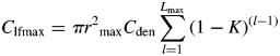
There is an upper limit on daily carbon fixation in the model imposed by the maximum effective leaf carbon. Maximum effective leaf carbon represents the limitation on light interception imposed by shoot architecture. Maximum effective leaf carbon (C_lfmax) is the carbon equivalent of the leaf area corresponding to the product of the maximum canopy radius, maximum leaf area index, and the sum of the light incident on the canopy layers:

(4)

where C_den in leaf carbon per unit area (leaf carbon concentration per leaf area per unit leaf mass), L_max is maximum leaf area index, K is the light extinction coefficient, and r_max is maximum canopy radius. Note that individual leaves are not explicitly modelled – rather, the total size and age distribution of the pool of leaf carbon is modelled.

It is assumed that acquisition of carbon and phosphorus per unit carbon in the acquiring organ changes only as a result of phosphorus depletion and tissue ageing, and the parameters that govern these processes in the model are calculated on the basis of specific leaf area (SLA) and specific root length (SRL), which are assumed to be constant. This assumption is made for the sake of simplicity and because no data showing changes of both SRL and SLA in Arabidopsis are available.

Resource allocation

The carbon required for maintenance respiration is removed from the pool of acquired carbon before carbon is allocated for other processes. Maintenance respiration for each organ class is the product of the carbon pool and maintenance respiration rate of that organ class. The only exception to this rule is maintenance respiration for leaves, which is calculated in an analogous fashion to carbon acquisition, scaling A_t between the leaf maintenance respiration (R_lf) and the ‘old’ leaf maintenance respiration, given by the product of R_lf and the fractional rate for ‘old’ leaf organs (R_oldlf).

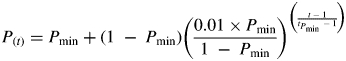
Allocation to reproduction is zero until time of initiation of reproductive growth (T₁), and increases in a linear fashion to reach unity at the time vegetative growth terminates (T₂). While allocation to reproduction is less than unity, the remainder is allocated to vegetative growth as described below. The time between T₁ and T₂ was also limited to a set value, T_D. Small values of T_D (T_D ≤ 20) force a rapid and complete switch to reproductive growth, while large values of T_D (T_D ≥ 40) permit (but do not force) an extended period of both reproductive and vegetative growth.

The partitioning of resources between root and shoot growth is broadly similar to the model of Reynolds and Thornley (1982). At each time step, newly acquired carbon is pooled with any carbon that was not utilized in growth or metabolism in the previous time step, and the carbon required for maintenance metabolism is removed from this pool. The newly acquired phosphorus is similarly pooled with any unused phosphorus remaining from the previous time step. The ratio of available carbon to available phosphorus, normalized by the phosphorus and carbon allocation to growth in the previous time step (referred to here as the internal resource ratio, Z_int) determines the ratio of allocation to root and shoot.

(5)

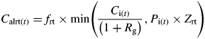
C_i is the pool of internally available carbon, P_i is the pool of internally available phosphorus, C_{al(t − 1)} and P_{al(t − 1)} are the carbon and phosphorus allocation to growth in the previous time step. The fraction of resources allocated to roots (f_rt) is given by:

(6)

where f_rep is the allocation fraction to reproductive organs, and Z_int is given by eqn (5). The fraction of resources allocated to stems and leaves is similar to eqn (6), but Z_int in the numerator is replaced by the inverse of Z_int. For Z_int > 1, available carbon is in excess, growth is limited by phosphorus, and root growth is favoured. For Z_int < 1, available phosphorus is in excess, growth is limited by carbon, and stem and leaf growth are favoured.

Organ growth

The carbon and phosphorus allocated to each organ class (root, stem, leaf, reproductive tissue and seeds) is incorporated into new tissue of each type on the basis of the C : P ratio and the carbon requirement for growth respiration of that organ class. The growth of the root carbon pool [C_alrt(t)] is given by:

(7)

where R_g is the growth respiration rate, Z_rt is the root C : P ratio. Growth of other organs is analogous, but growth of stems and leaves is controlled by the allocation fraction to stems and leaves (f_sht) which is further divided between the fraction to stem (f_stem) and the fraction to leaves (1 – f_stem). Since carbon and phosphorus allocation to the organ classes is based on the ratio of overall carbon and phosphorus allocation in the previous time step, and the incorporation of carbon and phosphorus into each organ class depends on the C : P ratio of that organ class, there may be excess carbon or phosphorus that is not incorporated into new growth. In addition, there is a maximum rate of leaf growth, above which any carbon or phosphorus allocated to leaf growth is considered to be in excess. Any excess carbon or phosphorus resulting from these factors is stored until the next time step, when it is included in the C_i or P_i terms in the calculation of Z_int.

A fixed proportion of resources allocated to reproduction are converted into mature seed (f_sd), after a time delay (T_sd) representing the time required for floral growth, pollination, and seed maturation. Viable seed is the cumulative sum of the product of allocation to seed and the probability of surviving at each time step.

Survival

Survival was modelled by considering mortality to be a sigmoidal function with half-maximum and steepness parameters, normalized by mortality at 120 d:

(8)

where g_S is a steepness parameter, k_S is the half-minimum, and t₀ is the time at which survival = 0. In effect, the first 100 d of a logistic curve that could be longer than 100 d is considered. For this reason the half-maximum parameter for the sigmoidal mortality function (k_S) may not correspond to 50 % survival. Three survival scenarios, with k_S values of 69, 79 and 89, which corresponded to 50 % survival to 68, 76 and 84 d were considered (see Fig. 2). These scenarios are referred to as S68, S76 and S84.

Fig. 2.

Three survival scenarios used in the sensitivity analysis, with 50 % probability of survival to 68, 76 and 84 d.

Senescence

There are two processes in the model for senescence and reallocation of resources in the leaf organ category. The model considers two pools in the leaf organ category: ‘new’ leaf organs, for which the carbon fixation rate exceeds the respiration rate, and ‘old’ leaf organs, for which the respiration rate exceeds the carbon fixation rate. The senescence of these pools is distinct. In both cases, there is a pool of leaf resources that cannot be reallocated (the fixed leaf fraction, f_fix), and leaf resources in excess of the fixed leaf fraction are reallocated at a specified rate (D). Carbon and phosphorus in the ‘old’ leaf pool are subject to reallocation (controlled by the above-mentioned rules) as leaf resources enter this pool. Conceptually, this mimics the ageing and senescence of individual leaves. Senescence of the ‘new’ leaf organ category mimics the programmed senescence of the entire canopy. This process begins at a specified time (T₃) and proceeds at the specified rate of senescence. Removal of carbon and phosphorus from the two leaf organ pools caused by reallocation from senescent tissue is accounted for in later time steps in the calculation of carbon acquisition and maintenance metabolism of the leaf organ class. It is assumed that programmed senescence does not begin until after initiation of reproductive growth (T₃ ≥ T₁).

Senescence of both leaf pools can also be altered by metabolic demand. If the carbon demand for maintenance exceeds the available carbon, the rate of senescence of the ‘old’ leaf organ category is increased to free enough carbon to meet the respiratory demand (up to a specified maximum rate, D_max). If increasing the rate of senescence of the ‘old’ leaf pool is insufficient to meet respiration demands, the ‘new’ leaf organ category senescence rate is increased, even before T₃, up to the specified maximum. Carbon and phosphorus are reallocated from these pools at each time step after senescence begins at a fixed rate, so that the reallocation of carbon and phosphorus from leaves decays in an exponential fashion. Note that all senescence processes deal with reallocation of resources, but do not consider abscission of organs – it is assumed that all organs are retained.

Optimization

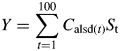
The model was optimized over the three phenology parameters that control initiation of reproduction (T₁), termination of vegetative growth (T₂) and initiation of programmed senescence (T₃), to find the phenology that resulted in the maximum size of the pool of realized (surviving to seed maturity) seed carbon, Y, which was used as a measure of yield:

(9)

Since the parameters to be optimized were phenological parameters, they could only take integer values, as the time step of the model is 1 d. These parameters were allowed to have any integer value between 20 and 100 d, subject to the limits discussed above (T₃ ≥ T₁, T₂ ≥ T₁, T₂ ≥ T₁ + T_D).

To characterize the response of seed carbon (Y) to the phenology parameters, all possible values of the three parameters were tested for the base high- and low-phosphorus cases (Fig. 3). These both showed a pronounced main peak with several local optima on the main peak, but in neither case were there isolated local optima apart from the main peak. We were not confident that standard optimization routines would be appropriate for this model, given that we wished to optimize for integer values. To avoid the computational load of testing all possible combinations of T₁, T₂ and T₃ (>100 000 combinations), all other cases were optimized using a two-step optimization process, with the first step designed to find the main peak, and the second step to find the true maximum.

Fig. 3.

The effect of reproductive phenology on seed production (seed carbon) of simulated Arabidopsis in high-phosphorus (A) and low-phosphorus (B) conditions. Increasing seed production is shown as increasing lightness, and the contour interval is 25 mg. Optimal phenology (indicated by *) occurred on a relatively smooth peak, which was later and lower in low phosphorus than in high. Termination of vegetative growth was constrained to be within 10 d of initiation of reproduction.

First, the entire range of possible values for initiation of reproduction (T₁) and termination of vegetative growth (T₃) were tested using a coarse step of 9 d. For each combination of T₁ and T₂, the optimal initiation of senescence (T₃) was determined using the coarse step of 9 d to cover the entire range of possible values followed by testing all values in a 16-d window centred on the maximum seed carbon value from the coarse step test. The optimal T₁ and T₂ values were similarly found using a second testing of all possible T₁ and T₂ values in a 16-d window centred on the maximum seed carbon value from the coarse step testing of T₁ and T₂ values. In practice, this procedure required about 6000–8000 iterations of the model (a 12- to 14-fold reduction from all possible combinations) to find the optimal phenology.

The sensitivity of the model to input parameters was analysed in several ways. Since the major cost to delayed reproduction was expected to be increased risk of mortality, optimal phenology was compared in two environments, high phosphorus (20 µm) and low phosphorus (1 µm), and for three survival scenarios with phosphorus-uptake parameters (maximum uptake rate – P_max, minimum uptake rate – P_min, and time of minimal uptake – t_Pmin), corresponding to five values of effective diffusion rate (D_e) of phosphorus in soil (see the Appendix). The survival scenarios ranged from 50 % survival at 84 d to 68 d (Fig. 2), and the phosphorus-uptake parameters corresponded to D_e from 1 × 10⁻⁹ to 1 × 10⁻⁷ cm² s⁻¹ (8·64 × 10⁴ to 8·64 × 10⁶ μm² d⁻¹), the range reported by Schenk and Barber (1979)

To determine sensitivity of plant growth and allocation simulated by the model to the parameters used, each parameter was varied by 10 % above and below the base value, and the optimal phenology and yield were determined for that scenario.

To estimate the relative importance of the various differences between plants from high- and low-phosphorus environments the parameters that differed between the high- and low-phosphorus scenarios were examined. Ten parameters differed between high- and low-phosphorus scenarios, two of which were parameters of phosphorus availability (P_max and P_min), and the remaining eight were plant physiological parameters (Z_rt, Z_stm, Z_lf, Z_rep, Z_sd, f_sd, f_fix, G_max; for definitions, see Table 3). To understand the impact of the differing parameters of plant physiology on simulated growth in the high- and low-phosphorus scenarios, both the high- and low-phosphorus scenario values of each in a scenario were tested with intermediate values for the other four differing parameters. The mean of the high- and low-phosphorus values of a parameter were used for the intermediate value, which corresponded to differences of 20–37 % from the original values (Table 4). First the model was optimized with the combination of all eight intermediate values for the physiology parameters for the high- and low-phosphorus scenarios. Then each of the eight parameters was altered singly to its corresponding high- and low-phosphorus values, and the model optimized for the high- and low-phosphorus scenarios. The effects of the phosphorus availability parameters were tested in a similar manner, by optimizing with each parameter at the corresponding high- or low-phosphorus scenario value while the other was set at a central value. The intermediate values used for the phosphorus availability parameters represented an increase or decrease of 11 % (for low- or high-phosphorus environments, respectively). For P_min, the minimum phosphorus-uptake parameter, the 11 % difference corresponded to a value intermediate between the high- and low-phosphorus values. Since the maximum phosphorus uptake rate (P_max) differed by nearly an order of magnitude (Table 3), a single intermediate value for this parameter was not used, but rather the parameter value was increased (for low phosphorus) or decreased (for high phosphorus) by 11 % to facilitate comparison between parameters.

Table 4.

Main model predictions were generally similar to observed data for Arabidopsis

Parameter	High phosphorus	Low phosphorus
(A) Model results
Base parameters
T1 (d)	34	50
T2 (d)	41	60
Yield (mg C)	218·6	155·1
Total carbon (mg)	1050	1150
Means (s.e.) from sensitivity analysis
T1 (d)	34·1 (0·13)	49·7 (0·39)
T2 (d)	41·3 (0·12)	59·7 (0·46)
Yield (mg C)	222 (3·02)	158 (2·37)
(B) Observed values (mean and s.e.)
Nord and Lynch (2008)
Bolting (d)	34·8 (1·3)	40·4 (1·6)
Total carbon (mg C)	1146 (71·7)	791 (64·4)
Yield (mg C)	175·7 (17·6)	131·4 (12·2)
E. A. Nord and J. P. Lynch (unpubl. res.)
Bolting (d)	44·0 (2·3)	47·3 (2·0)
Total carbon (mg C)	1001 (176)	1126 (113)

Base parameters are reflected in Table 3.

The sensitivity analysis involved 116 scenarios in which individual parameters were increased or decreased by 10 % while the others were held constant.

Parameterization

In principle, this model should be widely applicable to monocarpic annuals. Here a parameterization of the model for Arabidopsis thaliana is presented. Most of the necessary parameters were estimated from published reports (see Table 3), and several were calculated from data collected in an earlier experiment (Nord and Lynch, 2008).

Validation

The model predictions were validated against two sets of experimental results for A. thaliana grown in high- and low-phosphorus soils (Table 4). The first set was from an earlier experiment (Nord and Lynch, 2008), and the second set was from an unpublished experiment in which A. thaliana was grown with high or low phosphorus in elevated or ambient CO₂; here only the ambient CO₂ results are considered. The code for this model, along with an example input file, is available at: http://roots.psu.edu/phenology.

RESULTS

The model results were generally consistent with experimental data, predicting that low phosphorus availability delays flowering and reduces yield (Table 4). In general, the model predicted longer delay in flowering than was observed (16 d vs. 3–6 d). However, the range of age at flowering in the experimental data (35–44 d for low, and 40–47 d for high phosphorus) nearly overlapped with the model predictions (34 d and 50 d for low and high phosphorus), so that simulated phenology was slightly earlier than that observed in high-phosphorus and slightly later than that observed in low-phosphorus soils (Table 4).

Patterns of plant growth and partitioning predicted by the model were consistent with experimental observations. The sigmoidal carbon accumulation curves generated by the model (Fig. 4A, B) resemble plant growth curves. Simulated plant carbon accumulation (used as an analogue of biomass) was broadly similar to both experimental results for high phosphorus, but agreed better with the low-phosphorus results from the second experiment (Table 4). The model also predicted increased relative biomass allocation to roots in low-phosphorus conditions (Fig. 4A, B), as expected. Model plants balanced acquisition of carbon and phosphorus during vegetative growth by allocating resources to acquisition of the limiting resource, and any excess of carbon or phosphorus that carried over from one time step to the next was very small (Figs 4 and 5). However, once reproductive growth began, model plants could no longer balance carbon and phosphorus acquisition effectively, since shoot and root growth became limited by reproductive growth. As a consequence, model plants in low phosphorus accumulated excess quantities of phosphorus during reproductive growth (Fig. 5B).

Fig. 4.

Allocation and growth as simulated by the model in two scenarios: (A) 20 µm (high) phosphorus and (B) 1 µm (low) phosphorus. These are based on the standard parameters (Table 3), with D_e = 1·0 × 10⁻⁸ cm² s⁻¹, and optimal phenology. The dashed curve represents the probability of survival to a given age for scenario S76. The vertical dotted lines represent the initiation of reproduction and termination of vegetative growth from the optimal phenology. With high phosphorus the optimal phenology was: initiate reproduction at 34 d and terminate vegetative growth at 41 d. With low phosphorus these values were 50 and 60 d. Delaying reproduction in low phosphorus permitted enough additional phosphorus accumulation to offset the reduced probability of survival. Plants in low phosphorus can reach a similar size to those in high phosphorus, but are less likely to survive long enough to do so.

Fig. 5.

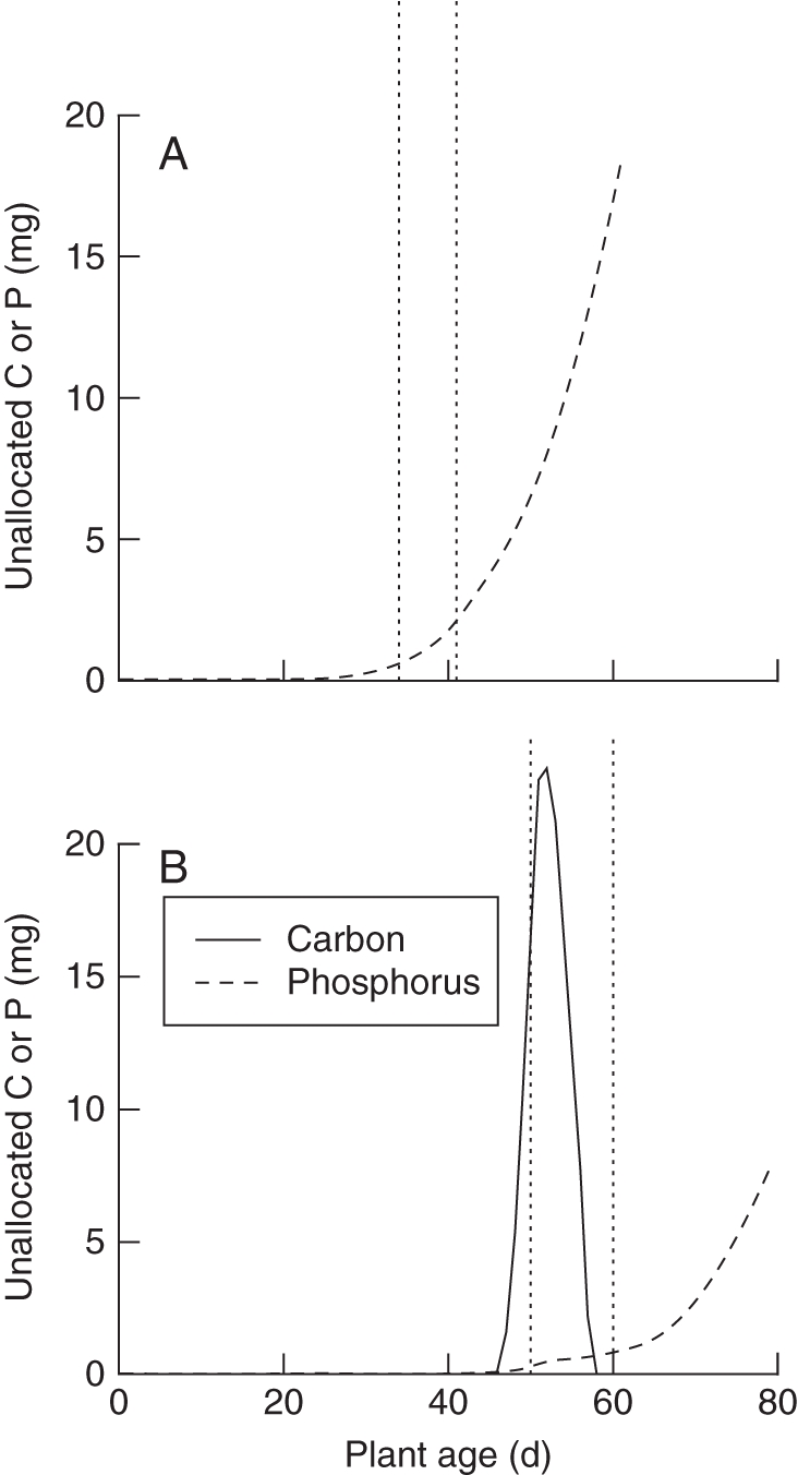
Unallocated carbon and phosphorus as simulated by the model in (A) 20 µm (high) phosphorus and (B) 1 µm (low) phosphorus. Unallocated carbon and phosphorus (as indicated) accumulate after reproductive growth begins, because the plant has fewer resources to allocate to vegetative growth and so is less able to balance acquisition of resources. Unallocated resources from one time step are allocated in the following time step. The vertical dotted lines represent the initiation of reproduction and termination of vegetative growth from the optimal phenology.

Phosphorus availability, phosphorus mobility and probability of survival influenced model plant phenology and yield in different ways (Fig. 6). The optimal phenology under low phosphorus was consistently later than that for high phosphorus in all of the 15 combinations of survival probabilities and phosphorus mobility (effective diffusion coefficient, D_e) values simulated. This delay in reproduction under low phosphorus was sensitive to phosphorus mobility (Fig. 6A), with delays increasing from about 10 d with D_e values of 3 × 10⁻⁷ to nearly 40 d with D_e values of 3 × 10⁻⁹. The probability of survival barely affected the optimal timing of reproduction; only under low phosphorus with the lowest D_e value (3 × 10⁻⁹) did probability of survival affect optimal phenology (Fig. 6A). Yield was more sensitive than phenology to probability of survival. Yield decreased when probability of survival declined earlier in the season (Fig. 6B). D_e had little effect on yield under high phosphorus, but decreasing D_e dramatically reduced yield under low phosphorus (Fig. 6B).

Fig. 6.

Effect of probability of survival and phosphorus diffusivity on optimal age of initiation of reproduction (A) and yield (B) for simulated Arabidopsis in low (1 µm; LP) and high (20 µm; HP) phosphorus. Simulations were carried out over a range of values of the effective phosphorus diffusion coefficient (D_e; 1·0 × 10⁻⁹ to 1·0 × 10⁻⁷ cm² s⁻¹, or 8·64 × 10⁴ to 8·64 × 10⁶ μm² d⁻¹) and with 3 survival scenarios with 50 % probability of surviving to: 84, 76 or 68 d (S84, S76 and S68). Survival scenario affected yield more than phenology. D_e affected both yield and phenology in low phosphorus, but had little effect in high phosphorus.

Optimal phenology and yield as simulated by the model were sensitive to several of the input parameters (Fig. 7). The sensitivity of a parameter in the model if a 10 % change in that parameter yielded a change in response of >5 % is reported. In general, yield responses were larger than phenology responses; no parameters produced changes of >17 % in phenology, while three parameters affected yield by at least 20 %. Increasing the maximal carbon assimilation rate (A_max) increased yield substantially (Fig. 7A, B). Increasing the conversion of reproductive organs into seed (f_sd), increasing the time to half-minimum for the decline in carbon assimilation with leaf age (increasing k_A) and increasing the carbon assimilation of reproductive tissue (A_rep) caused minor (5–10 %) increases in yield. Decreasing the respiration rate of reproductive tissue (R_rep) or the time lag required for seed to mature (T_sd) also caused minor (5–10 %) increases in yield. These are all factors which increase either resource acquisition or conversion of resources into yield. There was only one parameter to which both high- and low-phosphorus model plants were sensitive: increasing the maximum carbon assimilation rate (A_max) accelerated reproduction in both cases.

Fig. 7.

Sensitivity of yield (A, B) and phenology (C, D) to variation of input parameters for simulated growth with 20 µm (high) phosphorus (A, C) and 1 µm (low) phosphorus (B, D). The parameter ratio (on the abcissa) is the ratio of the parameter value used to the base parameter value (Table 3). For brevity, parameters with similar responses have been grouped together. The ordinate in all panels is the fractional difference in the response (fractional difference of 0·3 = 30 % increase). Parameter names and values are listed in Table 3.

There were several differences between high- and low-phosphorus scenarios in sensitivity of yield to input parameters. The largest difference was that an increase in maximum canopy radius (r_max) caused larger yield increases under high phosphorus than under low phosphorus (>20 % in high- vs. <10 % in low phosphorus; Fig. 7A, B). Reducing the maintenance respiration rate of leaves (R_lf) or the fraction of carbon and phosphorus in leaves that could not be reallocated at senescence (f_fix) caused modest increases in yield with high but not with low phosphorus. Reducing the phosphorus content of leaves (increasing Z_lf) resulted in modest increases in yield in the low-, but not in the high-phosphorus scenario. These differences reflect the carbon limitation of model plants with high phosphorus and the phosphorus limitation under low phosphorus. Delaying the decrease in probability of survival (increasing k_S) caused greater increases in yield in the low- than in the high-phosphorus scenario (approx. 30 % vs. < 10 %), reflecting the earlier optimal phenology in the high-phosphorus scenario.

The eight plant parameters that differed between high- and low- phosphorus plants (Z_rt, Z_stm, Z_lf, Z_rep, Z_sd, f_sd, f_fix, G_max) had important impacts on optimal phenology and yield when compared with a hypothetical plant with intermediate parameter values (Table 5). The effect of all the plant parameter differences together was substantial, and was very favourable for plants in the low-phosphorus scenario, increasing yield by 58 %, but unfavourable for plants in the high-phosphorus scenario, causing a 17 % decrease in yield. The single parameters which most affected yield differed for the high- and the low-phosphorus scenarios. Under high phosphorus, the largest yield decrease was caused by the increase in the fraction of leaf carbon and phosphorus which was not available for reallocation (f_fix). Under low phosphorus, the two greatest increases in yield were caused by increases in the C : P ratio in leaves and roots (Z_lf, Z_rt). With high phosphorus, none of the individual parameters caused changes of >5 % in phenology, and all of them together only delayed the initiation of reproduction by 1 d (6·25 %). With low phosphorus, several parameters caused changes in phenology of > 5 %, and all of them together accelerated phenology by 15 %.

Table 5.

Effect of parameters differing between high and low phosphorus simulated Arabidopsis in low (1 µm) and high (20 µm) phosphorus conditions

Differing parameter (% difference)	High phosphorus			Low phosphorus
	T1	T2	Yield	T1	T2	Yield
None*	32 d	41 d	263 mg	59 d	63 d	97·9 mg
% change caused by varying each differing parameter alone
Zrt (33 %)	–3·13	0	0·26	–3·39	–6·35	16·9
Zlf (37 %)	0	2·44	–3·48	–8·47	–6·35	28·8
Zrep (20 %)	0	0	–0·88	–3·39	1·59	5·41
ffix (21 %)	–3·13	–2·44	–11·4	0	–3·17	2·97
Gmax (33 %)	0	–4·88	–1·26	–5·08	4·76	1·79
% change caused by using LP and HP values for all differing parameters†
All differences	6·25	0	–16·8	–15·3	–4·76	58·3
% change from using central values for each differing phosphorus availability parameter
Pmax (11 %)‡	–3·13	0	–1·23	–10·2	0	21·6
Pmin (11 %)‡	0	0	–0·55	–5·08	0	11·6

Data shown are phenology and yield for the case where all plant parameter are equal and only phosphorus availability differs (row 1, in days and mg), the percentage change from these results when each single plant parameter is varied (rows 2–6), and the percentage change when all parameters that differ between high- and low-phosphorus plants are varied (row 7) – note that this case is the same as the baseline scenario used for the sensitivity analysis. Rows 8 and 9 are the percentage change when a central value is used for each of the phosphorus availability parameters.

* Only two phosphorus availability parameters differ between high and low phosphorus.

^† Differing parameters include the above plus Z_stm, Z_sd and A_rep. This is equivalent to comparing the baseline scenarios from the sensitivity analysis (represented in Fig. 3) with the scenarios in row 1 of this table, where only phosphorus availability differs.

^‡ For P_min, the central value was 0·885, and the HP and LP values were 11 % above and below. For P_max, the LP value was increased and the HP value reduced by 11 % to facilitate comparison with P_min.

Differences in phosphorus availability caused larger differences in phenology and yield than differences in localized phosphorus depletion caused by reduced D_e (Table 5). A central value of 0·885 for the fraction of initial phosphorus uptake still available after 15 d increased yield by 12 % and accelerated reproduction (T₁) by 5 % in the low-phosphorus scenario. A similar increase (11 %) in initial phosphorus uptake (P) increased yield by 22 % and accelerated reproduction (T₁) by 10 % under low phosphorus. However, similar decreases in these parameters had little effect under high phosphorus, with yield responses < 2 %, and only one phenology response, which was <4 %.

Low-phosphorus plants allocated relatively more resources to roots, and consequently root respiration was a greater fraction of total respiration (Fig. 8). Since the relative metabolic load of stems and leaves hardly differs between the low- and high-phosphorus scenarios, the greater respiratory cost of roots in low phosphorus reduces the ability of the plant to produce and support reproductive tissue. The metabolic load of roots and reproductive tissue was altered by phosphorus diffusivity in low phosphorus, with root metabolic costs increasing substantially for phosphorus diffusivity below 1·0 × 10⁻⁸ (Fig. 8).

Fig. 8.

Phosphorus diffusivity affects respiration of the organ classes as a fraction of total respiration in simulated Arabidopsis in low (1 µm; LP) and high (20 µm; HP) phosphorus. Simulations were carried out over a range of values of the effective phosphorus diffusion coefficient (D_e; 1·0 × 10⁻⁹ to 1·0 × 10⁻⁷ cm² s⁻¹, or 8·64 × 10⁴ to 8·64 × 10⁶ μm² d⁻¹) with 50 % probability of surviving to 76 d (S76). In both high and low phosphorus, shoot respiration was fairly constant. In low phosphorus, root respiration was relatively greater at lower levels of D_e, and this was offset by reduced respiration of reproductive tissue.

DISCUSSION

The model presented here captures many of the essential features of growth and partitioning of resources among root, shoot, and reproductive tissue in phosphorus-stressed plants. Simulated low-phosphorus plants were smaller in size than simulated high-phosphorus plants at any age, but with proportionally larger roots (Fig. 4). Simulated low-phosphorus plants consistently reproduced later than simulated high-phosphorus plants in 15 scenarios of survival probability and phosphorus mobility (Fig. 5). This highlights the trade-off faced by plants in low phosphorus; if the marginal decrease in survival is greater later in the season, the cost of delaying reproduction increases (Figs 2 and 4) later in the season.

The insensitivity of phenology and yield under high phosphorus to mobility of phosphorus in soil (D_e) is unsurprising – in high-phosphorus environments, growth should be limited by carbon, not by phosphorus. The near-insensitivity of phenology in high phosphorus to probability of survival is somewhat surprising. Under high phosphorus, phenology is sufficiently early that even in the earliest risk scenario (S68), phenology is essentially unaffected (Fig. 6A). In contrast, because optimal phenology under low phosphorus is generally later than in high-phosphorus, it is slightly more sensitive to changes in probability of survival, especially at lower levels of D_e (Fig. 6A). As a consequence, we hypothesize that plants adapted to soil environments in which phosphorus is less mobile should exhibit more phenological delay in response to low-phosphorus conditions than plants in more benign environments.

The extreme suppression of growth under low phosphorus with very low D_e highlights the important role root metabolic costs play in the optimization of plant phenology (Figs 6B and 8). Under these conditions, simulated plants acquired about 2 % of the resources they could acquire at higher D_e. Phosphorus availability was so low in these scenarios that a large fraction of plant resources was allocated to roots, and fewer resources to stem and leaves. This increased root respiration, and reduced resources available for reproductive growth. This is in agreement with other reports of the importance of root respiration, especially in low-phosphorus environments (Amthor, 1989; Fan et al., 2003; Lynch and Ho, 2005).

The plant parameter which most affected phenology was A_max, the maximum assimilation rate; increasing A_max accelerated reproduction in our model. Increased leaf level photosynthesis, equivalent to A_max in the model, generally increases in response to elevated CO₂ (Korner, 2006). Plant phenological responses to elevated CO₂ are somewhat variable (Nord and Lynch, 2009), but there are many reports of accelerated phenology, which would be consistent with the results of our model (Johnston and Reekie, 2008).

Substantial differences exist between the physiology of plants growing in high- and low-phosphorus conditions (Table 3). By varying each of these individually it was found that, of all the parameters that differed between these conditions, the leaf C : P ratio (Z_lf) had the greatest effect on yield and phenology in low phosphorus (Table 4), increasing yield by nearly 30 %. In general, the traits expressed in low phosphorus were beneficial in that environment when compared with a (hypothetical) phenotype intermediate to those of high and low phosphorus, increasing yield by over 58 %. In contrast, the traits expressed in high phosphorus were not beneficial when compared with the intermediate phenotype, decreasing yield by nearly 17 %. This suggests that plants might actually be better optimized for low phosphorus environments, which is consistent with the fact that low phosphorus availability is the primary constraint to plant growth in most terrestrial ecosystems (Lynch and Deikman, 1998).

Since metabolic costs influence yield (i.e. yield was sensitive to respiration rates of leaves and reproductive organs; Fig. 7A, B), the absence of leaf abscission in the model may be problematic, as a pool of old, inefficient leaf tissue continues to burden the plant. However, if this were the case, yield or phenology would be expected to respond to changing the fractional rate of respiration for old leaves (R_oldlf), which it did not. It is assumed that there is no remobilization of resources from roots, and root loss to herbivory or pathogens was not considered. Given the metabolic cost of maintaining roots and the reduced acquisition of phosphorus by older roots, root turnover could reduce the metabolic cost of root maintenance with little effect on phosphorus acquisition. Future extensions of this model could test the effect of root turnover on phosphorus acquisition, root respiration and reproductive phenology.

This model assumes that the C : P ratio of organs is fixed, though tissue phosphorus concentration varies with time (Nord and Lynch, 2008; Fig. 7). Furthermore, internal phosphorus redistribution is important in low-phosphorus environments (Wissuwa, 2003). These factors should permit greater growth in low-phosphorus conditions than the model predicts, since the sensitivity analysis (Fig 7) suggests that the C : P ratio of leaves influenced yield in low-phosphorus conditions. Future work with this model might involve testing the effect of allowing the C : P ratios to vary.

The model also assumes static A_max, P_max and respiration rates, but these are known to exhibit ontogenetic variability (Drouet et al., 2004). An alternate model was tested, in which specific root length (SRL) and, thus, P_max was allowed to vary through time, and the basic results were broadly similar to those presented here, with delays of 3–8 d in phenology compared with the fixed SRL model (data not shown). The simpler model presented here is preferable because the data required for parameterization are more readily available and because the more complex model would require excessive time to optimize the phenology.

The root and shoot partitioning based on increasing the acquisition of the limiting nutrient, ‘balanced growth’ (Davidson, 1969), is a central assumption of this model. While this may be an oversimplification (Reich, 2002), it reproduces the essential features of the regulation of root and shoot partitioning by phosphorus availability. However, this approach seems preferable to some of the optimization-based partitioning models, as it is based only on current conditions (Reynolds and Chen, 1996). We note that this approach may not be applicable to nutrients other than phosphorus and nitrogen, which both regulate root and shoot partitioning (Marschner, 1995).

The prevalence of low-phosphorus soils globally, and the emerging evidence of the alteration of plant phenology in response to global climate change suggests that phenological responses of plants to low-phosphorus environments may be important for the adaptation of plants to a changing climate. Lengthened growing seasons resulting from global change may allow increased phenological delay, which could benefit plants in low-phosphorus soils. However, changes in patterns of precipitation are likely to increase the risk of drought in some areas, which may increase risk of mortality. Finally, we note that low phosphorus availability is a primary constraint to the productivity of low-input agroecosystems (Lynch, 2007). Understanding the role of phenology in adaptation to low-phosphorus soils may be beneficial in efforts to develop crop varieties suited to low-input agricultural systems and crop varieties that allow reduced loss of phosphorus from agricultural soils (Karpinets et al., 2004), as well as in the effort to understand the influence of global climate change on plant growth and productivity (Lynch and St Clair, 2004; Nord and Lynch, 2009).

In conclusion, it has been shown here that delayed reproduction, which has been observed in plants growing in low-phosphorus soil, can be understood as a beneficial response that allows for increased acquisition and utilization of phosphorus. However, the benefit a plant is able to derive from delaying reproduction in low-phosphorus conditions is limited by the mobility (effective diffusion coefficient) of phosphorus in the soil, and the temporal distribution of mortality risk.

APPENDIX: Parameters used in the Barber–Cushman model

The Barber–Cushman model was used to estimate phosphorus-uptake parameters for specific soil conditions. Phosphorus uptake was simulated over 15 d, and then the output used to calculate the maximal phosphorus-uptake rate (mg P mg root C⁻¹ d⁻¹) when a root grows into new soil, and the fractional phosphorus-uptake efficiency of roots at ages 2–15 d

	Low P (1 µm phosphorus)
De	1·0 × 10−9	3·0 × 10−9	1·0 × 10−8	3·0 × 10−8	1·0 × 10−7
p.rteffmin	0·550	0·650	0·800	0·913	0·940
p.Pavail	2·09 × 10−3	2·83 × 10−3	3·66 × 10−3	4·21 × 10−3	4·34 × 10−3
p.rteffmintime	15	15	15	15	15
	High P (20 µm phosphorus)
De	1·0 × 10−9	3·0 × 10−9	1·0 × 10−8	3·0 × 10−8	1·0 × 10−7
p.rteffmin	0·700	0·903	0·968	0·985	0·987
p.Pavail	2·20 × 10−2	2·29 × 10−2	2·33 × 10−2	2·37 × 10−2	2·38 × 10−2
p.rteffmintime	15	15	15	15	15

Derived by fitting an exponential decay curve to the output from the Barber–Cushman model using these inputs

Name	Value	Units	Description and source
Km	5·25 × 10−3	μM	From Narang et al. (2000)
Imax	5·25 × 10−7	μmol cm−2 s−1
Cmin	9·60	nm
Ro	0·00865	cm	Initial root radius (Nord and Lynch, 2008)
R1	0·33	cm	Half-distance between root axes, default value
Cli	1·0	μm	Initial phosphate concentration
b	200		Buffer power of the soil; lower values did not permit growth when phosphorus concentration was 1 µm.
Vo	5·00 × 10−7	ml cm−2 s−1	Max water flow rate, default value. Model sensitivity to this parameter is low for phosphorus (Barber, 1995).
k	0·00	cm s−1	Root growth rate, zero because only depletion effects are required

Note: K_m and I_max differed for HP and LP, but the model is not particularly sensitive to them (Barber, 1995), so mean values were used.

LITERATURE CITED

- Aerts R. Nutrient resorption from senescing leaves of perennials: are there general patterns? Journal of Ecology. 1996;84:597–608. [Google Scholar]
- Aerts R, Chapin FS. The mineral nutrition of wild plants revisited: a re-evaluation of processes and patterns. Advances in Ecological Research. 2000;30:1–67. [Google Scholar]
- Aerts R, Bakker C, de Caluwe H. Root turnover as a determinant of the cycling of C, N, and P in a dry heathland ecosystem. Biogeochemistry. 1992;15:175–190. [Google Scholar]
- Amir S, Cohen D. Optimal reproductive efforts and the timing of reproduction of annual plants in randomly varying environments. Journal of Theoretical Biology. 1990;147:17–42. [Google Scholar]
- Amthor JS. Respiration and crop productivity. New York, NY: Springer-Verlag; 1989. [Google Scholar]
- Araujo AP, Teixeira MG, de Almeida DL. Variability of traits associated with phosphorus efficiency in wild and cultivated genotypes of common bean. Plant and Soil. 1998;203:173–182. [Google Scholar]
- Barber SA. Soil nutrient bioavailability: a mechanistic approach. 2nd edn. New York, NY: John Wiley & Sons; 1995. [Google Scholar]
- Beaver JS, Rosas JC, Myers J, et al. Contributions of the bean/cowpea CRSP to cultivar and germplasm development in common bean. Field Crops Research. 2003;82:87–102. [Google Scholar]
- Callahan HS, Pigliucci M. Indirect consequences of artificial selection on plasticity to light quality in Arabidopsis thaliana. Journal of Evolutionary Biology. 2005;18:1403–1415. doi: 10.1111/j.1420-9101.2005.00963.x. [DOI] [PubMed] [Google Scholar]
- Cohen D. Maximizing final yield when growth is limited by time or by limiting resources. Journal of Theoretical Biology. 1971;33:299–307. doi: 10.1016/0022-5193(71)90068-3. [DOI] [PubMed] [Google Scholar]
- Cohen D. The optimal timing of reproduction. American Naturalist. 1976;110:801–807. [Google Scholar]
- Comerford NB. Soil phosphorus bioavailability. In: Lynch JP, Deikman J, editors. phosphorus in plant biology: regulatory roles in molecular, cellular, organismic, and ecosystem processes. Rockville, MD: American Society of Plant Physiologists; 1998. pp. 136–147. [Google Scholar]
- Cordes EE, Bergquist DC, Shea K, Fisher CR. Hydrogen sulphide demand of long-lived vestimentiferan tube worm aggregations modifies the chemical environment at deep-sea hydrocarbon seeps. Ecology Letters. 2003;6:212–219. [Google Scholar]
- Cordes EE, Arthur MA, Shea K, Arvidson RS, Fisher CR. Modeling the mutualistic interactions between tubeworms and microbial consortia. Plos Biology. 2005;3:e77. doi: 10.1371/journal.pbio.0030077. doi:10.1371/journal.pbio.0030077. [DOI] [PMC free article] [PubMed] [Google Scholar]
- Davidson RL. Effect of root/leaf temperature differentials on root/shoot ratios in some pasture grasses and clover. Annals of Botany. 1969;33:561–569. [Google Scholar]
- Drouet JL, Pages L, Serra V. Dynamics of leaf mass per unit leaf area and root mass per unit root volume of young maize plants: implications for growth models. European Journal of Agronomy. 2004;22:185–193. [Google Scholar]
- Fairhurst T, Lefroy R, Mutert E, Batjes NH. The importance, distribution and causes of P deficiency as a constraint to crop production in the tropics. Agroforestry Forum. 1999;9:2–8. [Google Scholar]
- Fan MS, Zhu JM, Richards C, Brown KM, Lynch JP. Physiological roles for aerenchyma in phosphorus-stressed roots. Functional Plant Biology. 2003;30:493–506. doi: 10.1071/FP03046. [DOI] [PubMed] [Google Scholar]
- Fisher MCT, Eissenstat DM, Lynch JP. Lack of evidence for programmed root senescence in common bean (Phaseolus vulgaris) grown at different levels of phosphorus supply. New Phytologist. 2002;153:63–71. [Google Scholar]
- Florez-Sarasa ID, Bouma TJ, Medrano H, Azcon-Bieto J, Ribas-Carbo M. Contribution of the cytochrome and alternative pathways to growth respiration and maintenance respiration in Arabidopsis thaliana. Physiologia Plantarum. 2007;129:143–151. [Google Scholar]
- Gordon W, Jackson RB. Nutrient concentration in fine roots. Ecology. 2000;81:275–280. [Google Scholar]
- Gungula DT, Kling JG, Togun AO. CERES-maize predictions of maize phenology under nitrogen-stressed conditions in Nigeria. Agronomy Journal. 2003;95:892–899. [Google Scholar]
- Heemst HDJv. Plant data values required for simple crop growth simulation models: review and bibliography. 1988 Wageningen: Centre for Agrobiological Research. [Google Scholar]
- Hensel LL, Grbic V, Baumgarten DA, Bleecker AB. Developmental and age-related processes that influence the longevity and senescence of photosynthetic tissues in arabidoposis. The Plant Cell. 1993;5:553–564. doi: 10.1105/tpc.5.5.553. [DOI] [PMC free article] [PubMed] [Google Scholar]
- Iwasa Y. Dynamic optimization of plant growth. Evolutionary Ecology Research. 2000;2:437–455. [Google Scholar]
- Iwasa Y, Roughgarden J. Shoot root balance of plants: optimal-growth of a system with many vegetative organs. Theoretical Population Biology. 1984;25:78–105. [Google Scholar]
- Johnston A, Reekie E. Regardless of whether rising atmospheric carbon dioxide levels increase air temperature, flowering phenology will be affected. International Journal of Plant Sciences. 2008;169:1210–1218. [Google Scholar]
- Karpinets TV, Greenwood DJ, Ammons JT. Predictive mechanistic model of soil phosphorus dynamics with readily available inputs. Soil Science Society of America Journal. 2004;68:644–653. [Google Scholar]
- Kooijman SALM. Dynamic energy and mass budgets in biological systems. Cambridge: Cambridge University Press; 2000. [Google Scholar]
- Korner C. Plant CO2 responses: an issue of definition, time and resource supply. New Phytologist. 2006;172:393–411. doi: 10.1111/j.1469-8137.2006.01886.x. [DOI] [PubMed] [Google Scholar]
- Lynch JP. Roots of the second green revolution. Australian Journal of Botany. 2007;55:493–512. [Google Scholar]
- Lynch J, Deikman J. Phosphorus in plant biology: regulatory roles in molecular, cellular, organismic and ecosystem processes. Rockville, MD: American Society of Plant Biologists; 1998. [Google Scholar]
- Lynch JP, Ho MD. Rhizoeconomics: carbon costs of phosphorus acquisition. Plant and Soil. 2005;269:45–56. [Google Scholar]
- Lynch JP, St Clair SB. Mineral stress: the missing link in understanding how global climate change will affect plants in real world soils. Field Crops Research. 2004;90:101–115. [Google Scholar]
- Ma QF, Longnecker N, Atkins C. Varying phosphorus supply and development, growth and seed yield in narrow-leafed lupin. Plant and Soil. 2002;239:79–85. [Google Scholar]
- Manske GGB, Ortiz-Monasterio JI, Van Ginkel M, et al. Traits associated with improved P-uptake efficiency in CIMMYT's semidwarf spring bread wheat grown on an acid Andisol in Mexico. Plant and Soil. 2000;221:189–204. [Google Scholar]
- Marschner H. Mineral nutrition of higher plants. London: Academic Press; 1995. [Google Scholar]
- Narang RA, Bruene A, Altmann T. Analysis of phosphate acquisition efficiency in different arabidopsis accessions. Plant Physiology. 2000;124:1786–1799. doi: 10.1104/pp.124.4.1786. [DOI] [PMC free article] [PubMed] [Google Scholar]
- Nord E, Lynch J. Delayed reproduction in Arabidopsis thaliana improves fitness in soil with suboptimal phosphorus availability. Plant, Cell & Environment. 2008;31:1432–1441. doi: 10.1111/j.1365-3040.2008.01857.x. [DOI] [PubMed] [Google Scholar]
- Nord E, Lynch J. Plant phenology: a critical controller of soil resource acquisition. Journal of Experimental Botany. 2009;60:1927–1937. doi: 10.1093/jxb/erp018. [DOI] [PubMed] [Google Scholar]
- Pigliucci M, Schlichting CD. Reaction norms of Arabidopsis (Brassicaceae). 3. Response to nutrients in 26 populations from a worldwide collection. American Journal of Botany. 1995;82:1117–1125. [Google Scholar]
- R Development Core Team. R: a language and environment for statistical computing. 2008 Vienna: R Foundation for Statistical Computing. http://www.r-project.org/ [Google Scholar]
- Reekie EG, Bazzaz FA. Reproductive effort in plants. 3. Effect of reproduction on vegetative activity. American Naturalist. 1987;129:907–919. [Google Scholar]
- Rees M, Sheppard A, Briese D, Mangel M. Evolution of size-dependent flowering in Onopordum illyricum: a quantitative assessment of the role of stochastic selection pressures. American Naturalist. 1999;154:628–651. doi: 10.1086/303268. [DOI] [PubMed] [Google Scholar]
- Reich PB. Root-shoot relations: optimality in acclimation and adaptation of the ‘emperor's new clothes’? In. In: Waisel Y, Eschel A, Kafkafi U, editors. Plant roots – the hidden half. New York, NY: Marcel Dekker; 2002. pp. 205–220. [Google Scholar]
- Reynolds JF, Chen JL. Modelling whole-plant allocation in relation to carbon and nitrogen supply: coordination versus optimization. Plant and Soil. 1996;185:65–74. [Google Scholar]
- Reynolds JF, Thornley JHM. A shoot–root partitioning model. Annals of Botany. 1982;49:585–597. [Google Scholar]
- Rossiter RC. Phosphorus deficiency and flowering time in subterranean clover Trifolium subterraneum. Annals of Botany. 1978;42:325–330. [Google Scholar]
- Schenk MK, Barber SA. Phosphate uptake by corn as affected by soil characteristics and root morphology. Soil Science Society of America Journal. 1979;43:830–880. [Google Scholar]
- Shepherd KD, Cooper PJM, Allan AY, Drennan DSH, Keatinge JDH. Growth, water-use and yield of barley in Mediterranean-type environments. Journal of Agricultural Science. 1987;108:365–378. [Google Scholar]
- Snapp S, Lynch JP. Phosphorus distribution and remobilization in bean plants as influenced by phosphorus nutrition. Crop Science. 1996;36:929–935. [Google Scholar]
- Stearns S. The evolution of life histories. Oxford: Oxford University Press; 1992. [Google Scholar]
- Stessman D, Miller A, Spalding M, Rodermel S. Regulation of photosynthesis during Arabidopsis leaf development in continuous light. Photosynthesis Research. 2002;72:27–37. doi: 10.1023/A:1016043003839. [DOI] [PubMed] [Google Scholar]
- Thornley JH. Model to describe partitioning of photosynthate during vegetative plant-growth. Annals of Botany. 1972a;36:419–430. [Google Scholar]
- Thornley JH. Balanced quantitative model for root–shoot ratios in vegetative plants. Annals of Botany. 1972b;36:431–441. [Google Scholar]
- Vasilas BL, Nelson RL, Fuhrmann JJ, Evans TA. Relationship of nitrogen-utilization patterns with soybean yield and seed-fill period. Crop Science. 1995;35:809–813. [Google Scholar]
- Wissuwa M. How do plants achieve tolerance to phosphorus deficiency? Small causes with big effects. Plant Physiology. 2003;133:1947–1958. doi: 10.1104/pp.103.029306. [DOI] [PMC free article] [PubMed] [Google Scholar]