Improved signal processing to detect cancer by ultrasonic molecular imaging of targeted nanoparticles

Abstract

In several investigations of molecular imaging of angiogenic neovasculature using a targeted contrast agent, Renyi entropy [] and a limiting form of Renyi entropy ($I_{f,\infty }$) exhibited significantly more sensitivity to subtle changes in scattering architecture than energy-based methods. Many of these studies required the fitting of a cubic spline to backscattered waveforms prior to calculation of entropy [either $I_f(r)$ or $I_{f,\infty }$]. In this study, it is shown that the robustness of $I_{f,\infty }$ may be improved by using a smoothing spline. Results are presented showing the impact of different smoothing parameters. In addition, if smoothing is preceded by low-pass filtering of the waveforms, further improvements may be obtained.

INTRODUCTION

We have reported previously on application of several “entropies” for molecular imaging of tumor neovasculature.1, 2, 3 These investigations extend the scope of earlier studies of molecular targeting4 in order to achieve greater sensitivity to the accumulation of molecularly targeted perfluorocarbon nanoparticles binding to sparse targeting sites in vivo. We propose that the development of novel types of signal processing schemes sensitive to the signatures of such nanostructures could enhance detectability in inherently noisy environments.1, 3 Moreover, these contrast agents have demonstrated therapeutic potential with the incorporation of drugs into their lipid outer layer. Thus successful concurrent development of contrast-agent and contrast-agent-detection technology would produce a “theragnostic” suitable for simultaneous ultrasonic monitoring and noninvasive treatment of cancer.5

Unlike the conventional application of entropy for post-processing,6 our analysis is based on application of a “boxcar,” or moving window, entropy analysis directly to backscattered radio frequency (RF) ultrasound segments for construction of entropy images. In this approach, each pixel corresponds to a windowed section of RF, and that pixel value is the entropy of the windowed RF. Compared with conventional gray scale, significant improvements in sensitivity of detection of nanoscale molecular imaging agents have been obtained.1, 2, 3 Moreover, the same boxcar analysis may be applied to obtain “energy” or “log-energy” images [Eq. 3], which are a generalization of conventional gray scale imaging. However, these are also usually less sensitive than their entropic counterpart. A qualitative basis for this outcome has been discussed previously based on the geometry of the high dimensional function space in which the digitized RF “lives.”7, 8 In very rough terms, the energy is the length of the n-dimensional vector representing the digitized waveform, whereas the entropic measures (specifically $H_f$) correspond to the logarithm of the volume of the n-dimensional rectangle subtended by this vector. While signal energies of waveforms backscattered from a biological specimen are usually constrained to lie on a thin spherical shell, and hence have roughly the same lengths, the phases of these vectors may vary significantly. Consequently, the volumes of the rectangles they subtend may vary from finite values to zero with the logarithms of these volumes varying from a finite value to minus infinity. This explains only the possibility of greater entropic sensitivity to subtle changes in scattering architecture. The realization of this possibility in any given experimental situation is another matter, requiring theoretical and numerical study and becoming worthwhile after the means of efficient and reliable calculation and scope of applicability of various entropic measures have been established by experiment.

Our most recent report described an entropy, $I_{f,\infty }$ [see Eq. 2], which may be calculated by an algorithm suitable for real-time implementation. There remains, however, room for significant improvement in the algorithm by suppressing noise. The purpose of the current study is to investigate the effect of replacing the simple cubic spline fit employed previously with an optimal smoothing spline algorithm.9 While this involves a sacrifice in speed (up to a factor of 10 to obtain optimum smoothing), a comparison of smoothed and unsmoothed $I_{f,\infty }$ results can be expected to shed light on impact of noise on the real-time (i.e., unsmoothed) results. From the standpoint of clinical relevance, the loss in speed will easily be recovered by speed improvements in the next generation of multi-core processors. Moreover, significant and unexpected advantages, beyond suppression of spurious critical points (we use the phrase “critical point” to refer to any time t at which $f\text{'}(t)=0$), follow from smoothing. As shown below for bandpass filtered RF, an optimal smoothing spline applied in conjunction with the $I_{f,\infty }$ algorithm provides a means to mask noise-dominated RF segments. Moreover, this masking is automatic in the sense that it follows from the choice of signal-to-noise ratio (the $\delta y_i$ discussed in the following text) and the optimality of the smoothing fit. There is no need for choice of a signal-to-noise cutoff criterion.

While this study is based on a relatively large cohort of animals divided into positive and negative control groups, our primary goal is to compare the effects of different types of signal processing on the robustness of nanoparticle detection using backscattered RF. This is accomplished in a multistep process involving, first, the production of either entropy or energy images followed by, second, analysis of these images to extract a single number used to decide whether or not nanoparticle accumulation has occurred. The post-processing is based on the cumulative distribution function (CDF) of either the entropy or energy images and is completely free of subjective hand-drawn regions of interest (ROI). The CDF is used to segment the image into two parts, those either below (corresponding to pixels in the image containing nanoparticles) or above (corresponding to pixels in the image not containing nanoparticles) a certain analysis threshold (this process is described in the following text in connection with Fig. 8). This threshold is the only free parameter in our analysis, and our approach is to essentially evaluate all of them. Qualitatively, we define robustness of a signal processing scheme as insensitivity to choice of analysis threshold. The summary findings of this study are that application of bandpass filtering combined with fitting of optimal smoothing splines increases robustness of $I_{f,\infty }$ processing, application of bandpass filtering combined with fitting of optimal smoothing splines does not increase robustness of $\log [E_f]$ processing, and $I_{f,\infty }$ is more robust than $\log [E_f]$ processing.

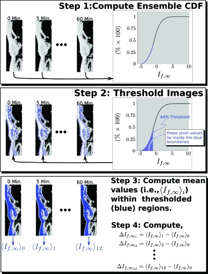
Figure 8.

Analysis steps for $I_{f,\infty }$ images from a single mouse. Step 1: the cumulative distribution function (CDF) of all 12 images aquired from the animal are computed. Step 2: The CDF is used to segment the image into targeted (inside the blue boundaries) and non-targeted (outside) segments according to pixel value being above or below the threshold level (44% in this case). Step 3: The mean value, $〈I_{f,\infty }〉{}_i$, of $I_{f,\infty }$ is computed for each “targeted region. Step 4: These are used to calculate $\Delta I_{f,\infty {}_i}=〈I_{f,\infty }〉{}_i-〈I_{f,\infty }〉{}_0$ for each time point in the study. This procedure is repeated for all mice in each group. An example of the resulting averages at each time point for two of the groups studied (using the 44% analysis threshold) is shown in Fig. 10, where the subscript i has been suppressed in $\Delta I_{f,\infty {}_i}$.

APPROACH

Our approach is based on the density function, $w_f(y)$ of the continuous function $y=f(t)$, assumed to underlie the sampled RF data. As described in previous studies, $w_f(y)$ corresponds to the density functions used in statistical signal processing.2 In contrast to statistical signal processing, $w_f(y)$ may be calculated directly from the measured “random” variable $f(t)$ using,

$$w_f(y)=\sum _{\{t_k|f(t_k)=y\}}1∕|f\text{'}(t_k)|,$$ (1)

where the domain of $f(t)$ has been mapped into the unit interval.

By a limiting procedure described in detail previously,3 we obtain a limiting form of the “Renyi” entropy

$$I_{f,\infty }=\log \left[\sum _{\{t_k|f\text{'}(t_k)=0\}}\frac{1}{|f″\left(t_k\right)|}\right],$$ (2)

which is one of the quantities investigated in this study.

Previous studies have shown that $I_{f,\infty }$ can be more sensitive to subtle changes in scattering architecture than what is found in more commonly used energy-based measures.1, 2, 3 We base our current study on a comparison of $I_{f,\infty }$ and $\log [E_f]$, which is given by

$$\log [E_f]=\log \left[\sum _{i=0}^{N}f{(t_i)}^2\mathit{dt}\right],$$ (3)

where N is the number of data points within our moving window ($N=128$ in the current study).

As will be shown in the following text (Figs. 45), optimal smoothing splines (when fit individually to filtered, boxcar-windowed data) are able to provide nearly complete suppression (i.e., masking) of noise-dominated RF segments, eliminating spurious ripple left over from frequency domain filtering and replacing it with a (to within floating point precision) completely flat baseline. As a result, the optimal smoothing spline may be used to automatically partition images into two parts: that which is composed of “real” signal and that where the returned echo is primarily noise. In the case of $I_{f,\infty }$, this is achieved by masking any return pixel where the sum appearing in the log of Eq. 2 is less than the double precision limit of the computer used to analyze the data (i.e., $\mathit{DBL}\_\mathit{EPSILON}$), which will happen for any RF segment that is flat. These pixels may then be excluded from all subsequent image post-processing. The same criterion is applied to the calculation of Eq. 3. Thus both the $I_{f,\infty }$ and $\log [E_f]$ results presented in the following text have been computed using the same thresholding condition.

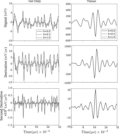
Figure 4.

Effects of smoothing parameter S on smoothed spline output for representative segments of unfiltered RF data.

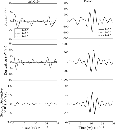
Figure 5.

Effects of smoothing parameter S on smoothed spline output for low-pass filtered versions of the same RF data shown in Fig. 4.

Numerical computation of $I_{f,\infty }$

Calculation of $I_{f,\infty }$ via Eq. 2 is accomplished by fitting a smoothing spline to the experimentally acquired data array using the algorithm described by Reinsch in 1967.9 Given a set of N values $y_i$ at times $t_i$, which in our case represent sampled points of representing backscattered RF between times $t_1$ and $t_N$, the corresponding smoothing spline approximation to those values is $g(t)$ minimizing

$${\int }_{t_1}^{t_N}{g}^{″}(t){}^2\mathit{dt},$$ (4)

subject to the constraint that

$$\sum _{i=0}^N\left(\frac{g(t_i)-y_i}{\delta y_i}\right)\le \hat{S},$$ (5)

where, operationally, $\delta y_i>0$ is the standard of deviation of the measured data point $y_i$ (taken to be $\delta y_i=0.002$ for our data sets using statistics from the water-only regions of our backscattered data). For aesthetic reasons, the smoothing parameter $\hat{S}$ is divided by the number of points, N to define a new smoothing parameter $S=\hat{S}∕N$. With this normalization, $S=0$ corresponds to no smoothing: the output of the algorithm is identical to a cubic spline fit. As $S\to \infty$, the output approaches the best fit line to the data. The optimum fit, corresponding to the minimum defined by Eqs. 4, 5 occurs somewhere near $S=1$.

As discussed by Reinsch, these equations may be combined into the problem of minimizing the functional

$${\int }_{t_0}^{t_N}{g}^{″}(t){}^2\mathit{dt}+p\{\sum _{i=0}^N\left(\frac{g(t_i)-y_i}{\delta y_i}\right)+z^2-S\},$$ (6)

where z is an auxiliary variable, which is needed in addition to the expected Lagrange multiplier p, since Eq. 5 is an inequality instead of an equality. Minimization with respect to p and z may be performed as described by Reinsch after writing $g(t)$ as a cubic spline and substituting this expression into Eq. 6 to obtain a $N\times N$ matrix minimization problem that may be solved iteratively. We have found, for the data presented in this study, that at most 10 (and on average 9) iterations are required to compute the optimal smoothing spline. As is often the case in matrix minimization problems, the solution requires use of an algorithm with an operation count of $N^3$ (in this case, Cholesky decomposition) at each iteration. Consequently, we expect the smoothing spline approach to be slower by a factor of $N^2$ than the simple cubic spline algorithm. In previous studies,2 upsampling of N to values of 4096 or 8192 was required to improve the accuracy of computed zeros of the derivatives of $f(t)$. In the current approach, this is not necessary, as described in the following text, so that $N=128$, thus mitigating the impact of Cholesky decomposition.

The resulting $g(t)$ will replace the raw time domain function, $f(t)$ appearing in Eqs. 2, 3.

The Reinsch algorithm computes the values of $g(t)$, $g\text{'}(t)$, and $g″(t)$ at the $t_i$. Thus it is easy to identify the location of critical points by finding zero crossings of the $g\text{'}(t)$ array and subsequently solving a quadratic equation. This is done as described in Press et al.10 (2nd ed., Chapt. 5, sect. 6) to avoid loss of precision. This also enables our implementation to return the locations of the critical points, and the values of the smoothing spline, and its first and second derivatives at these points.

MATERIALS AND METHODS

Nanoparticles for molecular imaging

For in vivo imaging, we formulated nanoparticles targeted to ${\alpha }_v{\beta }_3$-integrins associated with neovascularity in cancer by incorporating an “Arg-Gly-Asp” mimetic binding ligand into the lipid layer. Methods developed in our laboratories were used to prepare perfluorocarbon (perfluorooctylbromide, PFOB, which remains in a liquid state at body temperature and across the range of acoustic pressures used in this study11) emulsions encapsulated by a lipid-surfactant monolayer.12, 13 The nominal sizes for each formulation were measured with a submicron particle analyzer (Malvern Zetasizer, Malvern Instruments, Worcestershire, United Kingdom). Particle diameter distribution is unimodal with a peak measured at $200\pm 30$ nm.14

Animal model

The study was performed according to an approved animal protocol and in compliance with guidelines of the Washington University institutional animal care and use committee.

Human MDA 435 cancer cells were implanted in the inguinal fat pad of 15 athymic nude mice between 19 and 20 days prior to acquisition of data. Five of these animals were injected with ${\alpha }_v{\beta }_3$-targeted nanoparticles, five were injected with nontargeted nanoparticles, and five were injected with saline. In addition, 15 athymic nude mice not implanted with tumors were imaged in the same region following the same imaging protocol: five were injected with ${\alpha }_v{\beta }_3$-targeted nanoparticles, five were injected with nontargeted nanoparticles, and five were injected with saline. Mice were preanesthesitized with a ketamine/xylazine cocktail. Mice were then placed on a heated platform maintained at 37| °C and injected by tail vein with 0.030 ml ${\alpha }_v{\beta }_3$-targeted nanoparticle emulsion, 0.030 ml non-targeted nanoparticle emulsion, or 0.030 ml saline (equivalent to a whole body dose of approximately 1 ml/kg). Anesthesia was administered continually with isoflurane gas through a nose cone. Subsequently, ultrasound data were acquired at 0 through 60 mins in 5 min intervals. After the ultrasound data were collected, the tumor was extracted for histological staining. The entire procedure was approved by the Washington University animal care committee.

Ultrasonic data acquisition

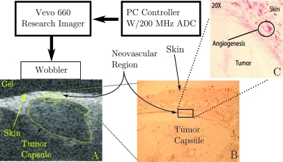
A diagram of our apparatus is shown in Fig. 1. RF data were acquired with a research ultrasound system (Vevo 660, Visualsonics, Toronto, Canada). The tumor was imaged with a 35 MHz center frequency single element “wobbler” probe, and the RF data corresponding to single frames were stored on a hard disk for later off-line analysis. The frames consisted of 384 lines of 2048 12-bit words acquired at a sampling rate of 200 MHz using a Gage 12400 digitizer card (connected to the analog-out and sync ports of the Vevo) in a controller PC. Each frame corresponds spatially to a region 1.5 cm wide and 0.8 cm deep. At the bottom left of Fig. 1 is a close-up schematic of the imaging probe and its relation to the coupling gel, skin, and tumor capsule. A conventional image from one of the mice used on our study is shown in this part of the figure. Also indicated is the region where neovasculature resulting from angiogenesis is present. As the figure indicates, significant neovasculature develops between skin and tumor capsule. This is due to recruitment of new vessels from the highly vascular skin. To the right of the close-up is an image of a histological specimen extracted from a mouse model. At the top of the slide is a section of skin (the elliptical structures in this area are hair follicles), below which is a thin angiogenic layer identified by immunohistochemical staining, and below that is a portion of the tumor capsule. The close proximity of neovasculature to the skin-transducer interface is one of the primary obstacles that must be overcome by any quantitative detection scheme intended to determine the extent of this region.

Figure 1.

A diagram of the apparatus used to acquire backscattered RF data, in vivo, (A) a typical ultrasonic gray scale image together with (B) a histologically stained section of the tumor indicating portions where ${\alpha }_v{\beta }_3$-targeted nanoparticles nanoparticles could adhere, and (C) a further enlarged section indicating more precisely the location of viable target sites (red by ${\beta }_3$ staining).

Ultrasonic data processing

A moving window analysis was performed on each waveform by moving a rectangular window (128 points long, 0.64 $\mu \mathrm{s}$) in 0.08 $\mu s$ steps (16 points), resulting in 121 window positions within the output data set. In previous investigations, we have found that choice of window length, which was constrained by digitizer sampling rate of 500 MHz, involves trade-offs between resolution and sensitivity. Larger window sizes tended to produce greater sensitivity at the expense of resolution with the optimum for these studies (found by experimentation) near 0.512 $\mu \mathrm{s}$ for window length and 0.064 $\mu \mathrm{s}$ for step size. Consequently, for this new study, performed using a 200 MHz digitizer, we chose values close to the “best” values used previously.

A smoothing spline was fit to each window. [We point out that we have applied the smoothing spline fit to each 128 point window and not to the entire 2048 point raw RF waveform because attempts to fit the entire waveform sometimes resulted in erroneous (i.e., complete) flattening of all portions of the 2048 point waveform occurring after the large echo from the water-tissue interface. The fitting routine also returned an array of first and second derivatives at the locations of any critical points in the window.] The arrays were used to compute $I_{f,\infty }$ according to Eq. 2. This produced an image for each time point in the experiment (i.e., 0, 5, …, 60 min).

Data analysis

RF waveform analysis

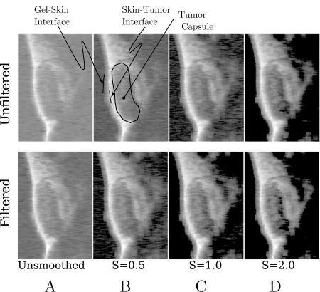
All RF data were processed off-line to reconstruct $I_{f,\infty }$ images. Total analysis time using the new algorithm was roughly 45 min on an eight core desktop computer (compared to less than 5 min for the cubic spline algorithm for $I_{f,\infty }$ and roughly 1 week for analogous $H_f$, or $I_f(1.99)$ analysis on a cluster of just over 20 computers that was reported previously2). A representative set of these images is shown Fig. 2. The top row shows $I_{f,\infty }$ images made using the raw backscattered RF acquired at 0 min post-injection of ${\alpha }_v{\beta }_3$-targeted nanoparticles (the direction of insonification is from the left). The results of no smoothing and smoothing using S ranging from 0.5 to 2.0 are shown. The gray scale lookup table used to make these figures has been inverted to match the display of conventional B-Mode gray scale images where interfaces are bright. This inversion between entropy and energy images has been observed in all previous studies.3 In all images, the gel-skin and skin-tumor interfaces are visible as is the tumor capsule (labeled in figure). We have also investigated the effects of lowpass filtering the raw entire 2048 point RF waveform prior to computation of $I_{f,\infty }$ and $\log [E_f]$ using the frequency-domain filter function $F(f)$ given by,

$$\begin{array}{c}F(f)=\frac{1}{4}(1.0+\tanh [a_l(f-f_{\mathit{lower\; cutoff}})])\times (1.0+\tanh [a_u(f_{\mathit{upper\; cutoff}}-f)]),\end{array}$$ (7)

where $a_l=0.75$, $a_u=0.25$, $f_{\mathit{lower\; cutoff}}=0$ MHz, and $f_{\mathit{upper\; cutoff}}=36$ MHz. The upper cutoff was chosen to correspond to the 6 dB point of our apparatus. This function, $F(f)$ has the shape of a smoothed rectangular window turning on near $f_{\mathit{lower\; cutoff}}$ and turning off near $f_{\mathit{upper\; cutoff}}$. The coefficients $a_l$ and $a_u$ govern the sharpness of these transitions. This function was chosen as a gate function because it is infinitely differentiable. We have investigated other window functions (various pole number Butterworth filters) and find that all perform in a roughly equivalent way. The second row shows $I_{f,\infty }$ images made using the lowpass filtered RF. As discussed following Eq. 3, pixels corresponding to noise are “masked.” These masked pixels are black in the images above (the gray scale look up table of which has been inverted to match the conventions used in medical ultrasonics). In both rows, there is an evident increase in the number of masked pixels as smoothing is increased. However, this trend is more pronounced in the second row, so that, surprisingly, for smoothing parameter $S=1.0$, there is a partitioning of the image into noise-dominated and signal-dominated portions. These masked pixels will be excluded from all subsequent analysis of the image.

Figure 2.

Subsets (middle portion: $0.75\times 0.55\hspace{1em}\mathrm{cm}$) of smoothing spline $I_{f,\infty }$ images based on unfiltered (top row) and low-pass filtered (bottom row) RF obtained from a MDA435-implanted mouse injected with ${\alpha }_v{\beta }_3$-targeted nanoparticles. (A) Smoothing parameter $S=0$, (B) $S=0.5$, (C) $S=1.0$, (D) $S=2.0$. The RF used to construct these images was acquired immediately after injection.

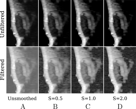
The same raw RF data were processed using Eq. 3 to construct $\log [E_f]$ images. These are shown in Fig. 3, which exhibits the same structures visible in Fig. 2. However, there are no masked pixels in any of these images and, consequently, no effective partitioning of image into signal- and noise-dominated portions.

Figure 3.

Subsets (middle portion: $0.75\times 0.55\hspace{1em}\mathrm{cm}$) of smoothing spline $\log [E_f]$ images based on unfiltered (top row) and low-pass filtered (bottom row) RF obtained from a MDA435-implanted mouse injected with ${\alpha }_{\upsilon }{\beta }_3$-targeted nanoparticles. (A) Smoothing parameter $S=0$, (B) $S=0.5$, (C) $S=1.0$, (D) $S=2.0$ The RF used to construct these images was acquired immediately after injection.

From Fig. 2 we may conclude that the combination of lowpass filtering prior to smoothing spline computation provides effective image partitioning into signal- and noise-dominant components. This is shown more clearly in Fig. 4. The top row shows unfiltered time domain segments extracted from a gel-path-only portion of data (left column) and RF backscattered from tissue (right column). Each panel contains three graphs corresponding to no smoothing (i.e.,$S=0.0$), $S=0.5$, and $S=1.0$ (near optimum according to Reinsch9), plotted as a function of time over a 0.32 μs window corresponding to half of our moving window length. The effects of smoothing are evident in the left panel. However, in the right panel, they are not because, operationally, the effect of smoothing is limited in magnitude by the value of $\delta y_i=0.002$ used in our data analysis (this value was measured from the experimental data by computing the standard deviation of the gel-only part of filtered RF for a representative subset of data sets). In the second row are the corresponding first derivative plots; the third row shows the corresponding second derivatives. As for the raw RF plots, the effects of smoothing are most evident in the lower amplitude plots from the gel-path-only segments of the backscattered RF.

The corresponding plots, using the same raw data after lowpass filtering as described in the preceding text, are shown in Fig. 5. The impact of the filtering is obvious in all plots as the water-only plots show total suppression of the signal for smoothing parameter $S=1.0$.

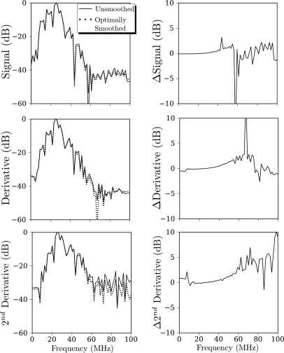
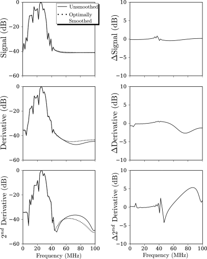
While we have adopted the current combination of low-pass filtering at the 6 dB point of our apparatus, followed by optimal smoothing spline fit, on the basis that all analysis parameters may be chosen objectively, it is possible that more aggressive low-pass filtering might achieve the same level of noise suppression. To evaluate this possibility, we have computed the Fourier transform magnitudes of two the traces shown in the left columns of Figs. 45 (the unsmoothed and the optimally smoothed). These are shown in Figs. 6 and 7, respectively.

Figure 6.

Effects of smoothing parameter S on smoothed spline output for unfiltered RF data. Left column: Comparison of log magnitude of Fourier transforms of smoothed (i.e., $S=1$) and unsmoothed (i.e., $S=0$) data from the left columns of Fig. 4. Right column: Plots of the unsmoothed log magnitude minus the smoothed log magnitude.

Figure 7.

Same comparison as Fig. 6 but applied to the low-pass filtered data of, Fig. 5.

The top row, left column, of Fig. 6 shows the magnitude of the Fourier transform of two of the unfiltered RF segments appearing in the top left panel of Fig. 4; immediately to the right of this panel is a plot of the unsmoothed magnitude minus the smoothed magnitude. The slight upward trend of this curve implies that the smoothing operation does perform some low-pass filtering, consistent with the smoothing observed in Fig. 4. However, this filtering is never more than 2.5 dB in magnitude, which is rather low for a typical low-pass filter. We ignore frequencies above 45 MHz because we have chosen to perform the Fourier transforms for this examination without use of window functions (e.g., a Hamming Window). Consequently, the discontinuity between initial and final points of the RF segments will introduce spurious energy in the higher frequencies. This is not a major concern because we are primarily interested in the behavior of the magnitude plots at or below 36 MHz. In the next two rows are similar plots for the first and second derivatives that are used in Eq. 2. In these panels, we also observe weak, low-pass filtering.

A similar comparison of magnitudes based on low-pass filtered RF is shown in Fig. 7. Comparing this figure with Fig. 6 shows that when applied to low-pass filtered RF, the optimal smoothing performs almost no low-pass filtering as indicated by the practically flat Δ curves in the right column of the figure. Moreover, whether or not the data are low-pass filtered, there is little difference in magnitudes of smoothed or unsmoothed data (top rows of Figs. 67). The effect of optimal smoothing is, however, discernable for the first and second derivatives as may be seen by comparing the second and third rows of Figs. 67. This may partially explain the results we will present in the following text that show that the combination of low-pass filtering of the entire RF waveform prior to optimal smoothing of the RF segments within the moving boxcar produces the greatest sensitivity to the presence of accumulating nanoparticles. However, we emphasize again that our primary motive for adopting this analysis strategy is that it allows for completely objective choice of all analysis parameters (in this case the low -pass cutoff frequency, which is measured experimentally, and the smoothing parameter, which is determined theoretically by the optimality criterion).

On the basis of these comparisons, we conclude that it is unlikely that more aggressive low-pass filtering could achieve the same level of noise suppression obtained using optimal smoothing splines. This observation has been tested by analyzing the data with low-pass cutoffs as low as 24 MHz. Thus it appears that in addition to making possible data analysis by purely objective means, the optimal smoothing spline analysis yields greater noise suppression than linear frequency-domain filtering. Perhaps this result is not too surprising given that Eq. 6 is manifestly nonlinear in its dependence on the input RF.

Image analysis

As stated previously, the segment of RF within the boxcar, or moving window, is processed either by Eq. 2 or (3) to produce a pixel value for either an $I_{f,\infty }$ or $\log [E_f]$ image. For each mouse used in this study, this is done using RF data acquired at $0,5,\dots ,60$ min post-injection to produce an image at each time point. For this study, in which the same portion of the anatomy was imaged at successive intervals, a major objective was to quantify changes in these image features as a function of time. Consequently, we require a means of identifying changes in the images. Because our goal is to identify and quantify the accumulation of targeted nanoparticles, which occurs preferentially at targeting sites, this suggests that segmenting the image into “targeted” and “non-targeted” regions will be required as part of the analysis. One of the chief goals of our research has been to develop objective algorithms that do not require user input (e.g., hand-drawn ROI).

Figure 8 displays the steps of such an algorithm graphically. For each mouse used in this study, a histogram of the image pixel values appearing over the entire time course (i.e., 0, 5, 10, …, 60 min) was constructed and normalized to obtain the probability density function (PDF) of these values and then integrated to obtain the CDF. This is shown in the top panel of the figure. Next, pixel values corresponding to “analysis thresholds” at the lower $2\%,4\%,\dots ,98\%$ of the CDF were then used to segment the images at each time point into two regions corresponding to targeted and “untargeted tissue.” The figure shows the segmentation for an example analysis threshold of 44%. The blue lines, shown in the second panel of the figure, indicate the boundary between targeted (inside the blue boundaries) and non-targeted (outside the blue boundaries) regions. Subsequently, the mean value of pixels in the targeted region are computed as a function of time post-injection. This is indicated in the bottom panel of the figure in which the mean value of $I_{f,\infty }$ found at each time, denoted in the figure by $〈I_{f,\infty }〉{}_i$, $i=1,\dots ,12$, is shown immediately below the thresholded image. Subsequently, the change in these mean values,

$$\Delta I_{f,\infty {}_i}=〈I_{f,\infty }〉{}_i-〈I_{f,\infty }〉{}_0,$$ (8)

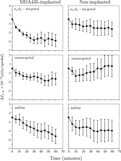
is computed ($\Delta I_{f,\infty {}_0}=0$). The analysis diagrammed in Fig. 8 was performed for all animals in all groups and the results averaged by group. We will drop the subscript i in the remaining discussion and refer only to the $\Delta I_{f,\infty }$. It is these $\Delta I_{f,\infty }$, for instance, that are plotted in Fig. 10, which is an example of the time course of $\Delta I_{f,\infty }$ corresponding to a 44% analysis threshold and which we will discuss in more detail shortly.

Figure 10.

(Color online) Average time course of $\Delta I_{f,\infty }$ images obtained from the five MDA435-implanted (left, top) and five non-implanted mice (right, top) injected with ${\alpha }_v{\beta }_3$-targeted nanoparticles, five MDA435-implanted (left, middle),and five non-implanted mice (right, middle) injected with non-targeted nanoparticles, and five MDA435-implanted (left, bottom) and five non-implanted mice (right, bottom) injected with saline. These data were obtained for the CDF threshold set to include the lower 44% of pixel values in the $I_{f,\infty }$ from each of the images in each group. Standard error bars for each group are also shown.

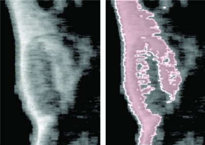
Before discussing results, we mention that we have verified that automatic segmentation based on the procedure of Fig. 8 is consistent with the biochemical processes underlying ${\alpha }_v{\beta }_3$-targeting. An example of this is shown in Fig. 9. The pixels colored red (using the procedure of Fig. 8) are in a region that are known from independent immunohistochemical assay to coincide with the region where ${\alpha }_v{\beta }_3$-targeted nanoparticles will accumulate. Moreover, the fact that the brightening is collocated with the tumor-skin interface is consistent with recruitment of angiogenic neovasculature from the highly vascularized skin where there is typically a relatively elevated amount of naturally occurring angiogenesis. However, it does raise the question about the source of image brightening observed in the MDA435-implanted mice that were injected with ${\alpha }_v{\beta }_3$-targeted nanoparticles. To address this concern, a second group of controls, non-tumor-implanted mice, were studied in three groups: five mice injected with ${\alpha }_v{\beta }_3$-targeted nanoparticles, five injected with non-targeted nanoparticles, and five injected with saline. As discussed in Sec. 4, for some analysis thresholds, there is a slight enhancement of the skin due to accumulation of ${\alpha }_v{\beta }_3$-targeted nanoparticles. However, both the rate of change and the maximum of $\Delta I_{f,\infty }$ are less than that occurring in MDA435-implanted mice, and significance is observed at different analysis thresholds than in the MDA435-implanted group injected with ${\alpha }_v{\beta }_3$-targeted nanoparticles, indicating that clinical detection of tumor associated angiogenesis using ${\alpha }_v{\beta }_3$-targeted nanoparticles is possible.

Figure 9.

Closeup of thresholded smoothing spline $I_{f,\infty }$ images. (Left) Image based on backscattered RF obtained from MDA435 tumor implanted mouse (same RF data used in Figs. 2345) immediately after injection of ${\alpha }_v{\beta }_3$-targeted nanoparticles. (Right) Image based on backscattered RF obtained from the same region 60 min after injection, “colorized” so that all pixels in the bottom 44% of the histogram (constructed using the 0-60 min $I_{f,\infty }$ images obtained from this mouse) are red.

RESULTS

Based on measured values reported in Figs. 56789, we first discuss $\Delta I_{f,\infty }$ results obtained using optimal smoothing splines (i.e., $S=1.0$) followed by an identical analysis performed without smoothing. Finally, we present the results of a analysis for $\Delta \log [E_f]$ using smoothing splines.

Typical evolution of $\Delta I_{f,\infty }$

Representative time course plots for the change in $I_{f,\infty }$ using the 44% analysis threshold are shown in Fig. 10 [we present this analysis threshold because it corresponds roughly to the maximum confidence value, defined in Eq. 9, obtained using $I_{f,\infty }$ analysis; see Figs. 12 or 15]. These plots compare the change in the average for the group of MDA435-implanted mice injected with ${\alpha }_v{\beta }_3$-targeted nanoparticles with the change in the average for the group of non-implanted mice injected with ${\alpha }_v{\beta }_3$-targeted nanoparticles (top row), the group of MDA435-implanted mice injected with non-targeted nanoparticles with the change in the average for the group of non-implanted mice injected with non-targeted nanoparticles (middle row), and the group of MDA435-implanted mice injected with saline with the change in the average for the group of non-implanted mice injected with saline (bottom row). The plots are representative of the result obtained over a broad range of analysis thresholds in showing that the group of MDA435-implanted mice injected with ${\alpha }_v{\beta }_3$-targeted nanoparticles exhibit a greater decrease in $I_{f,\infty }$ than does the group injected with non-targeted nanoparticles. Standard error bars are also shown on all plots and, typical for a broad range of CDF thresholds, in the MDA435-implanted mice injected with ${\alpha }_v{\beta }_3$-targeted nanoparticles, they are, on average, significantly smaller those in the control groups.

Figure 12.

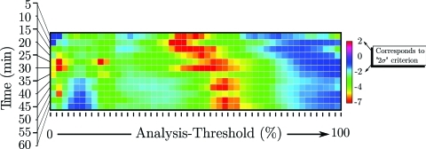
Confidence panel for ${\alpha }_v{\beta }_3$-targeted nanoparticle group processed using optimal smoothing splines applied to low-pass filtered RF data. This image is composed of data like that shown in the right side of Fig. 11.

Figure 15.

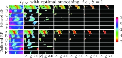
Confidence, c, panels from $\Delta I_{f,\infty }$ for all groups used in our study. Pixels with absolute value below $c=2,3,,7$ are masked (colored black). Panels A–F were obtained using unfiltered RF: (A) MDA435-implanted mice injected with ${\alpha }_v{\beta }_3$-targeted nanoparticles ($N=5$), (B) MDA435-implanted mice injected with non-targeted nanoparticles ($N=5$), (C) MDA435-implanted mice injected with saline ($N=5$), (D)–,(F) same injections into $N=5$ tumor-free mice. Panels A′ through B′ are the corresponding panels obtained using low-pass filtered RF. The smoothing spline parameter $S=1.0$ in all cases.

Global assessment of receiver performance: Confidence analysis

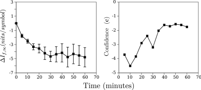
For the purposes of detection, it is actually the ratio of the mean value to the standard error that is significant. We have plotted an example of these ratios (for the MDA 435 implanted group injected with ${\alpha }_v{\beta }_3$-targeted nanoparticles) in the right panel of Fig. 11; the left-hand panel reproduces the plot shown in the upper right-hand corner of Fig. 10. To shorten subsequent discussion of our results, we will define this ratio (confidence) as15

$$c=\frac{\mathit{mean}}{\mathit{standard\; error}}.$$ (9)

As the left panel shows, for an analysis threshold of 44%, the mean value of $\Delta I_{f,\infty }$ is at all times roughly twice the standard deviation or more from zero.

Figure 11.

(Color online) Average time course of $\Delta I_{f,\infty }$ images obtained from the five MDA435-implanted mice injected with ${\alpha }_{\upsilon }{\beta }_3$-targeted nanoparticles and the corresponding confidence ratios (c) as a function of time post-injection. The left panel is the same panel appearing in the top right column of Fig. 10.

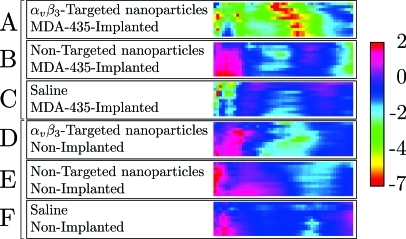
As stated in the preceding text, an analysis like that shown in Fig. 11 was performed for all even CDF thresholds between 0% and 98%. This enables a global evaluation of the performance of entropic and log-energy processing that is not compromised by use of subjective (e.g., hand-drawn) ROI, which we would like to stress are never employed in our analysis. A summary of all resulting values of c for the MDA435-implanted mice injected with ${\alpha }_v{\beta }_3$-targeted nanoparticles group is shown in image format in Fig. 12. The color of each pixel in this image is mapped from the value of c according to the calibration bar to the right of the image that shows that c ranges from the unit less values 2 to negative 7. While it is conventional in medical image processing to apply the “two-sigma” criterion to determine statistical significance (corresponding to $c=2$, emphasized by text label and arrows), it is possible that other criteria may be more suitable for specific applications. In this regard, the data contained in a “confidence” image such as Fig. 12 may be used to quickly assess the impact of different analysis thresholds (by masking all pixels above or below a given value of c, which is discussed in the following text) so that the sensitivity of $\Delta I_{f,\infty }$ at various analysis thresholds may be globally assessed.

$I_{f,\infty }$ confidence panels, like that shown in Fig. 12, have been made for all six groups used in our study. These are shown as a stack in Fig. 13 together with a color calibration bar. Inspection of the confidence stack shows that the top confidence panel corresponding to the MDA435-implanted group injected with ${\alpha }_v{\beta }_3$-targeted nanoparticle exhibits confidence ratios with the greatest magnitude.

Figure 13.

Confidence panel stack comprised of confidence panels for all groups processed using optimal smoothing splines applied to low-pass filtered RF data. This panel is comprised of confidence summary images like that shown in Fig. 12.

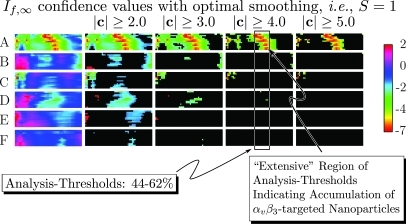
The use of masked confidence panels to establish selection criteria that uniquely identify the tumor-implanted group injected with targeted nanoparticles (to the exclusion of all other control groups) is demonstrated in Fig. 14. This array of confidence panels is our final form of display for results. We point out that it is a five-dimensional presentation having three dimensions within each confidence panel (i.e., post-injection time in the vertical direction, analysis threshold in the horizontal direction, and confidence c in the out-of-plane or color direction), another dimension for animal group (the vertical direction within the array), and a fifth dimension being the masking level for the absolute value of confidence ratio c (the horizontal direction within the array). Thus the unmasked color regions indicate analysis threshold/time combinations at which the mean value of $\Delta I_{f,\infty }$ is statistically different from zero according to the $\sigma =2,3,\dots ,7$ statistical criterion. In spite of the high dimensionality of the display, it permits rapid evaluation of $I_{f,\infty }$ or $\log [E_f]$ processing as well as the impact of various RF preprocessing steps, i.e., low-pass filtering or smoothing spline fitting. For instance, if we focus our attention on the column in the array labeled “$\left|c\right|=4$,” we observe in the top row an “extensive” (meaning contiguous, wider than three columns over at least half the height of the confidence panel) region near the middle of the panel corresponding to analysis thresholds centered around 54% (indicated in the figure by the labeled rectangle). The remaining confidence panels in this rectangle are devoid of extensive unmasked (i.e., not “blacked” out) regions in the same range of analysis thresholds. Consequently, the criteria $\left|c\right|=4$, with analysis threshold between 44% and 62%, becomes a means of distinguishing the targeted/tumor-implanted group from all others. We note that these criteria exhibit the presence of accumulating, targeted, nanoparticles within 5 min of injection.

Figure 14.

Confidence panel summary composed of confidence panel stacks for all groups, masked at successively greater confidence levels (labels A–F defined in Fig. 13). The left most (unmasked) stack of this image is shown in Fig. 13 and presents confidence panels in the same order. Also indicated is a conservatively chosen range of analysis thresholds (44%–62%) that produce an “extensive” region of confidence ratios, c, having an absolute value greater than 4 only for the tumor-implanted group injected with ${\alpha }_v{\beta }_3$-targeted nanoparticles. Thus this range of analysis thresholds combined with the requirement that $\left|c\right|\ge 4$ comprises selection criterion permitting identification of this group.

$I_{f,\infty }$ Confidence results

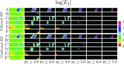
Figure 15 compares confidence arrays obtained using either low-pass filtered data (top half) or unfiltered data (bottom half). In this figure, the array includes masking levels ranging from $c=2,3,\dots ,7$. The fact that the color region in row A covers over two-thirds of the confidence image for $c=2,3$ and approximately 50% for $c=4$ indicates the robustness of the $\Delta I_{f,\infty }$ in the face of changing analysis thresholds. This observation is consistent with the partitioning into signal- and noise-dominated regions provided by the smoothing spline as discussed in Fig. 9.

The remaining rows, B–F, are composed of control group confidence panels: MDA 435 implanted mice injected with non-targeted nanoparticles in row B and MDA 435 implanted mice injected with saline in row C. Non-implanted mice injected with ${\alpha }_v{\beta }_3$-targeted nanoparticles, non-targeted nanoparticles, or saline are summarized in rows D, E, and F, respectively. These control group panels are composed of mostly masked pixels (i.e., masked analysis threshold/time combinations) for confidence $c=2$, while for $c=4$, all control groups are masked almost completely. Finally, we note that there are extensive ranges of analysis thresholds where the ${\alpha }_v{\beta }_3$-targeted/MDA 435 implanted panel is not masked, but where the corresponding pixels in the panels for the control groups are masked, implying that there exist ranges of analysis parameters where the incidence of “false” positives would be low. In fact, for the $c=4$ column, there are practically no color pixels below (i.e., in rows B–F) those appearing in row A, as discussed previously in connection with Fig. 14.

Confidence panels obtained using the same RF but without bandpass filtering prior to smoothing spline computation are shown in rows A′—F′. As for rows A–F, the smoothing parameter was set to $S=1$. We note that the color regions in row A are larger than those in row A′, while the color regions in rows B–F are typically smaller than those in B′F′, implying that the application of low-pass filtering of the raw RF prior to computation of smoothing splines can be used to increase chances of detecting true positives while reducing the probability of false positives.

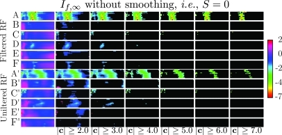
Figure 16 shows the same comparison shown in Fig. 15 for RF data segments that have not been smoothed. The confidence arrays indicate that the same criteria may be chosen to exclusively separate the tumor-implanted/targeted group from the controls: $\left|c\right|=4$ with analysis threshold between 44% and 62%. However, reference to the calibration bar shows that the low-pass filtering followed by smoothing spline fit analysis procedure achieves this with greater values of confidence.

Figure 16.

Confidence, c, panels from $\Delta I_{f,\infty }$ for all groups used in our study. Pixels with absolute value below $c=2,3,\dots ,7$ are masked (colored black). Panels A–F were obtained using unfiltered RF: (A) MDA435-implanted mice injected with ${\alpha }_v{\beta }_3$-targeted nanoparticles ($N=5$), (B) MDA435-implanted mice injected with non-targeted nanoparticles ($N=5$), (C) MDA435-implanted mice injected with saline ($N=5$), (D)–(F) same injections into $N=5$ tumor-free mice. Panels A′ through B′ are the corresponding panels obtained using low-pass filtered RF. The smoothing spline parameter $S=0$ in all cases.

log[E_f] confidence results

Corresponding results obtained using $\Delta \log [E_f]$ analysis are shown in Fig. 17. We note that the calibration bar in this figure spans values from 2 to −7, which is roughly the negative of the range of values spanned in Fig. 15. As discussed in the preceding text, this inversion is consistent with other studies.3

Figure 17.

$\Delta \log [E_f]$ confidence panels, corresponding to those shown in Fig. 15. Both figures were made using the same RF.

DISCUSSION

Application of bandpass filtering combined with fitting of optimal smoothing splines increases robustness of $I_{f,\infty }$ processing

We note that in Fig. 15 there are relatively few color pixels in the control confidence panels for masking levels $\left|c\right|>4$ and that above this level of masking the color regions in row A are much smaller in width (i.e., number of adjacent analysis thresholds) and that the color regions no longer have a single analysis threshold that extends from 5 to 60 min (i.e, it is not possible to draw a single vertical line from top to bottom of confidence panel A that lies exclusively within the unmasked region). We will take the width of the color region in confidence panel A, as a measure of robustness of $\Delta I_{f,\infty }$ analysis. Consequently we will limit our discussion of $\Delta I_{f,\infty }$ panels to the first four columns of the figure, where the analysis is “robust.”

Comparison of the widths of the color regions of the filtered of row A vs row A′, (Fig. 15) shows that they are wider in the filtered case for all masking levels $\left|c\right|\le 4$. This might have been anticipated from the $I_{f,\infty }$ images constructed using filtered vs unfiltered RF data (shown in Fig. 2) that exhibit a striking difference in the completeness of baseline suppression. As these “suppressed” pixels are excluded by automatic CDF-based analysis, the confidence panels of Fig. 15 are based on significantly different contributions from the backscattered RF. In the filtered case, these come almost exclusively from the signal-dominated portions of the RF, which, as Fig. 2 shows, correspond to the RF backscattered from tissue. The robustness is also influenced by differences in shape in the signal-dominated portions of RF. Comparison of the left columns of Figs. 45 reveal the values of the second derivatives in the optimal smoothing spline analysis, $g″(t)$ tends to be reduced, as we might expect, after filtering of higher frequencies. This will have the effect of increasing the magnitude of terms appearing in Eq. 2. Thus not only will there be a reduced contribution from non-tissue portions of backscattered RF, but contributions from RF backscattered from tissue will be larger after application of both filtering and spline smoothing. Both of the effects are consistent with the observed greater widths of the color regions in Row A vs Row A′ of Fig. 15, which demonstrates the greater robustness of the combination of bandpass filtering and fitting of optimal smoothing splines vs fitting of optimal smoothing splines alone.

Application of bandpass filtering combined with fitting of optimal smoothing splines does not increase robustness of log[E_f] processing

Inspection of the widths of columns A vs A′’, B vs B′, …, F vs F′ in Fig, 17 shows that (unlike Fig. 15) there is little difference between filtered and unfiltered results on a per group basis.

$I_{f,\infty }$ is more robust than log[E_f] processing

Using the same conventions as in the preceding text, comparison of the widths of unmasked regions in rows A and A′ in Figs. 1517 demonstrate that in the current study, $\Delta I_{f,\infty }$ is more robust than $\Delta \log [E_f]$ processing.

The results shown in Fig. 3 may provide a partial explanation. They show that there can be significant contribution from gel-only RF segments. The contribution of these segments will increase in importance as the analysis threshold is lowered. This points out a significant benefit offered by the masking observed with $\Delta I_{f,\infty }$ processing. When masking occurs the image CDF, which is the foundation for all subsequent processing of either $\Delta \log [E_f]$ or $\Delta I_{f,\infty }$ images, encodes effects almost exclusively from tissue, which is the only place in the image where the effects of targeted nanoparticle accumulation could possibly be measured. Without masking, the CDF must also account for the effects of noise. The impact this has on a confidence panel, such as that shown in the column labeled $c=4$ of Fig. 15, would be to combine the broad band of colored pixels into a narrower band of pixels having larger amplitude as observed in the corresponding column of Fig. 17.

It seems obvious that imposition of an additional masking step in the analysis of $\Delta \log [E_f]$ images could be used to reduce the impact of noise from noise-dominated segments of RF. However, the masking level would become an additional parameter in the analysis that would have to be chosen by imposition of additional assumptions on the data (e.g., choice of a signal-to-noise ratio cutoff level in addition to measurement of signal-to-noise ratio, which is essentially what we have done with the choice of $\delta y_i$). The advantage of $\Delta I_{f,\infty }$ processing is the economy of assumptions it affords, eliminating the need to choose the cutoff level by replacing it with the optimality criterion of the smoothing spline fit.

CONCLUSION

The confidence ratio analysis described in the preceding text has focused on robustly detecting accumulation of ${\alpha }_v{\beta }_3$-targeted nanoparticles in tumors at all CDF thresholds (0%–98%), while avoiding false positives in the control groups. This choice was made in order to identify a robust set of values for the confidence ratio and to execute a rigorous assessment of the utility of $I_{f,\infty }$ imaging of nanoparticle targeted neovasculature.

The results presented in this paper extend earlier studies where it was shown that entropy based measures, $H_f$, $I_f(r)$, and $I_{f,\infty }$, were able to detect targeted nanoparticles in tumor neovasculature.1, 2, 3, 8

References

- Hughes M. S., McCarthy J. E., Marsh J. N., Arbeit J. M., Neumann R. G., Fuhrhop R. W., Wallace K. D., Znidersic D. R., Maurizi B. N., Baldwin S. L., Lanza G. M., and Wickline S. A., “Properties of an entropy-based signal receiver with an application to ultrasonic molecular imaging,” J. Acoust. Soc. Am. 121, 3542–3557 (2007). 10.1121/1.2722050 [DOI] [PubMed] [Google Scholar]
- Hughes M. S., McCarthy J. E., Marsh J. N., Arbeit J. M., Neumann R. G., Fuhrhop R. W., Wallace K. D., Thomas T., Smith J., Agyem K., Znidersic D. R., Maurizi B. N., Baldwin S. L., Lanza G. M., and Wickline S. A., “Application of Renyi entropy for ultrasonic molecular imaging”, J. Acoust. Soc. Am. 125, 3141–3145 (2009). 10.1121/1.3097489 [DOI] [PMC free article] [PubMed] [Google Scholar]
- Hughes M. S., McCarthy J. E., Wickerhauser M., Marsh J. N., Arbeit J. M., Fuhrhop R. W., Wallace K. D., Thomas T., Smith J., Agyem K., Lanza G. M., and Wickline S. A., “Real-time calculation of a limiting form of the renyi entropy applied to detection of subtle changes in scattering architecture,” J. Acoust. Soc. Am. 126, 2350–2358 (2009). 10.1121/1.3224714 [DOI] [PMC free article] [PubMed] [Google Scholar]
- Hall C. S., Marsh J. N., Scott M. J., Gaffney P. J., Wickline S. A., and Lanza G. M., “Time evolution of enhanced ultrasonic reflection using a fibrin-targeted nanoparticulate contrast agent,” J. Acoust. Soc. Am. 108, 3049–3057 (2000). 10.1121/1.1322566 [DOI] [PubMed] [Google Scholar]
- Lanza G. M., Winter P. M., Caruthers S. D., Hughes M. S., Hu G., Schmieder A. H., and Wickline S. A., “Theragnostics for tumor and plaque angiogenesis with perfluorocarbon nanoemulsions,” Angiogenesis 13, 189–202 (2010). 10.1007/s10456-010-9166-0 [DOI] [PMC free article] [PubMed] [Google Scholar]
- Gull J. and Skilling S. F., “Maximum entropy method in image processing,” IEE Proc. F, Commun. Radar Signal Process. 131, 646–659 (1984). 10.1049/ip-f-1.1984.0099 [DOI] [Google Scholar]
- Hughes M. S., Marsh J. N., Hall C. S., Savy D., Scott M. J., Allen J. S., Lacy E. K., Carradine C., Lanza G. M., and Wickline S. A., “Characterization of digital waveforms using thermodynamic analogs: Applications to detection of materials defects,” IEEE Trans. Ultrason. Ferroelectr. Freq. Control 52, 1555–1564 (2005). 10.1109/TUFFC.2005.1516028 [DOI] [PubMed] [Google Scholar]
- Hughes M., Marsh J., Woodson A., Lacey E., Carradine C., Lanza G. M., and Wickline S. A., “Characterization of digital waveforms using thermodynamic analogs: Detection of contrast targeted tissue in MDA 435 tumors implanted in athymic nude mice,” in Proceedings of the 2005 I.E.E.E. Ultrasonics Symposium (2005) pp. 1609–1616. [DOI] [PubMed]
- Reinsch C.H., “Smoothing by spline functions,” Num. Math. 10, 177–183 (1967). 10.1007/BF02162161 [DOI] [Google Scholar]
- Press W. H., Teukolsky S. A., Vetterling W. T., and Flannery B. P., Numerical Recipes in C, 2nd ed. (Cambridge University Press, Cambridge, UK, 1992), pp. 113–116. [Google Scholar]
- Hughes M., Marsh J., Hall C., Fuhrhop R. W., Lacy E. K., Lanza G. M., and Wickline S. A., “Acoustic characterization in whole blood and plasma of site-targeted nanoparticle ultrasound contrast agent for molecular imaging,” J. Acoust. Soc. Am. 117, 964–972 (2005). 10.1121/1.1810251 [DOI] [PubMed] [Google Scholar]
- Flacke S., Fischer S., Scott M. J., Fuhrhop R. J., Allen J. S., McLean M., Winter P., Sicard G. A., Gaffney P. J., Wickline S. A., and Lanza G. M., “Novel MRI contrast agent for molecular imaging of fibrin implications for detecting vulnerable plaques,” Circulation 104, 1280–1285 (2001). 10.1161/hc3601.094303 [DOI] [PubMed] [Google Scholar]
- Lanza G. M., Wallace K. D., Scott M. J., Cacheris W. P., Abendschein D. R., Christy D. H., Sharkey A. M., Miller J. G., Gaffney P. J., and Wickline S. A., “A novel site-targeted ultrasonic contrast agent with broad biomedical application,” Circulation 94, 3334–3340 (1996). [DOI] [PubMed] [Google Scholar]
- Winter P., Caruthers S., Kassner A., Harris T., Chinen L., Allen J., Zhang H., Robertson J., Wickline S., and Lanza G., “Molecular imaging of angiogenesis in nascent vx-2 rabbit tumors using a novel αvβ3-targeted nanoparticle and 1.5 tesla MRI,” Cancer Res. 63, 5838–5843 (2003). [PubMed] [Google Scholar]
- Sackett D.L., “Why randomized controlled trials fail but needn’t: II. failure to employ physiological statistics, or the only formula a clinician-trialist is ever likely to need (or understand!),” Can. Med. Assoc. J. 165, 1226–1237 (2001). [PMC free article] [PubMed] [Google Scholar]