

Abstract
We report on the direct measurement of the exchange rate of waters of hydration in elastin by T2-T2 exchange spectroscopy. The exchange rates in bovine nuchal ligament elastin and aortic elastin at temperatures near, below and at the physiological temperature are reported. Using an Inverse Laplace Transform (ILT) algorithm, we are able to identify four components in the relaxation times. While three of the components are in good agreement with previous measurements that used multi-exponential fitting, the ILT algorithm distinguishes a fourth component having relaxation times close to that of free water and is identified as water between fibers. With the aid of scanning electron microscopy, a model is proposed allowing for the application of a two-site exchange analysis between any two components for the determination of exchange rates between reservoirs. The results of the measurements support a model (described elsewhere [1]) wherein the net entropy of bulk waters of hydration should increase upon increasing temperature in the inverse temperature transition.
1 Introduction
A well known characteristic of elastin, an insoluble protein that is responsible for the elasticity of vertebrate tissues, is that the complex microscopic solvent-protein relationship dictates its macroscopic behavior. For example, experimental measurements of the Youngs modulus demonstrated a dependence of the stress-strain relationship on solvent polarity [2] [3] [4] [5] [6] [7] [8]. The development of the remarkable resilience of the protein is believed to be correlated to the entropy change of elastin upon extension [1]. Using molecular dynamics simulations of a poly(GVGVP) peptide, it was shown that hydrophobic hydration is an important source of entropy based elasticity [9] [10]. Fundamental to the mechanical property of elastin is the inverse temperature transition — a process pointed out by D.W. Urry in numerous experimental studies of a poly(GVGVP) peptide [1] [11] [12] [13]. During the inverse temperature transition there is an increase in order of the backbone upon raising the temperature - microscopically a hydrophobic association of β turns occur, resulting in a macroscopic volumetric contraction. During the phase transition, structured hydration becomes less ordered bulk water due to the hydrophobic association of elastin β turns [1]. The goal of this work is to quantify in detail the exchange of waters of hydration in elastin and shed light on the complex water-protein association.
In this work, we implement a relatively new experimental technique known as relaxation exchange spectroscopy [14], [15]. This method allows for observing the displacement of mobile molecules over time between interconnected pores. The experiment involves correlating the spin-spin relaxation (T2) rates of mobile molecules over an experimentally variable mixing time. In the measurement, the spins of the ensemble are encoded and decoded by their T2 relaxation rates. Between the encoding and decoding stages the experimentally controlled mixing time allows us to track the displacement of molecules from one site to another. Central to the method is a 2D Inverse Laplace Transform (ILT) algorithm allowing for multi-exponential fitting to the data [16]. The net result of the 2D algorithm is a map of relaxation times with cross peaks indicating exchange between sites distinguishable by their T2 times.
Relaxation exchange spectroscopy has been implemented with success in a variety of porous systems. The method has been validated by considering a model porous medium consisting of mixtures of nonporous borosilicate and soda lime spheres in water [17]. In the measurement, the expected length scales between domains correlated well (within 25 percent) with that computed by the exchange time and molecular diffusion coefficient of water. A detailed analysis was recently presented on the 2D T2-T2 exchange experiment and applied successfully in white cement paste for extracting the exchange rates and an estimate of the pore sizes [18]. Recently, a novel propagator-resolved relaxation exchange experiment has been proposed by enabling spatial resolution together with T2-T2 exchange [15]. One of the challenges in two-dimensional relaxation exchange NMR is that the encoding times may be comparable to the exchange times. In order to analyze the resulting experimental data, in this limiting case, it is required that one perform simulations to determine quantitative information, such as the exchange rates [19]. Nevertheless, two dimensional relaxation exchange spectroscopy is quickly gaining popularity in applications where quantifying the details of exchange between reservoirs may prove to be significant in understanding connectivity and structure in a complex system.
The experimental data presented in this work highlight the mutual exchange between various sites in bovine nuchal ligament elastin and aortic elastin at temperatures below, near and at the physiological temperature. In both of the elastin samples, at all temperatures, we measure four clearly distinguishable relaxation rates corresponding to four discernable domains. A model is proposed, supported by SEM, where the waters of hydration in close proximity to the protein can be further divided into four groups that exchange with the three other components independently. Using this model, it is argued that a two-site exchange analysis may be performed for determining the exchange rates between the various reservoirs.
2 Materials and Methods
Purified bovine nuchal ligament and aortic elastin were purchased from Elastin Products Company (Elastin Products Co., Owensville, MO). The elastins were purified by the neutral extraction method of Partridge [20]. Two samples were made: (a) Nuchal Ligament Elastin (NLE) suspended in D2O and (b) Aortic Elastin (AE) suspended in D2O. The samples were prepared in a similar fashion: the elastin was immersed in abundant 99 percent D2O and was mixed with D2O by using a sonicator for 30 minutes (the temperature during this process was controlled to under 40°C), and then left at room temperature for more than 76 hours. The samples were then placed in standard 5mm NMR tubes and sealed using ethylene-vinyl acetate. The loss of water in any of the samples using this seal was less than 1 percent over the entire course of the experiments. Each sample was approximately 1.5 cm in length. The estimated concentration of elastin in D2O was 0.5g/ml.
All the experiments were carried out on a Varian Unity 200MHz NMR spectrometer using a Varian liquids NMR probe. The 90° pulse time on our system was 35μs. The effect of this pulse time on the signal is negligible as the timescale of the water dynamics studied was on the order of milliseconds. For the NLE sample, the experiments were conducted at 10, 25 and 37°C. The AE sample was studied at only 25°C. At each temperature a 2H 2D T1-T2 experiment and several 2H 2D T2-T2 experiments with different mixing times were carried out.
The NMR pulse sequence for the T1-T2 experiments is illustrated in Fig.1 [16]. In the experiments the magnetization is inverted by the first 180° pulse and then recovers towards thermal equilibrium with a relaxation time of T1 during a delay t1. The 90° pulse transforms the magnetization into the transverse plane and the NMR signal is detected by a CPMG pulse train [21]. The information regarding T1 is encoded by varying the delay time t1. Using a 2D ILT of the data, a T1-T2 correlation map is obtained. The caption in Fig.1 highlights the 4-step phase cycling scheme that was implemented.
Fig. 1.

RF pulse sequence used for 2D T1-T2 correlation experiments in this work. In the experiments phase cycling was ϕ1 = x, −x, ϕ2 = x, x, −x, −x, ϕ3 = y and the receiver phase was ϕReceiver = x, x, −x, −x. The experimental values for t1 and τ are described in the text.
The pulse sequence employed in T2-T2 experiments is illustrated in Fig.2 [15]. The sequence consists of two 180° pulse trains which allow for the encoding of T2 information before and after the mixing period. During the mixing time, denoted by tm, water molecules that migrate between different compartments experience different relaxation times before and after the mixing time. The are the apparent T2 times measured in the presence of exchange and are different from the T2 measured in the absence of exchange. The exchange is manifested into the 2D ILT map as a cross peak. Water that does not exchange between compartments is observed as a diagonal peak in the 2D ILT T2-T2 map as it only has one T2 throughout the entire experiment. A 4-step phase cycle, shown in the caption in Fig.2, was used to eliminate the undesired signal that is built up during the mixing time. By incrementing the mixing time, a series of T2-T2 maps were obtained and the exchange of water between different compartments in elastin was studied via the time dependence of the cross peak intensities.
Fig. 2.

RF pulse sequence used for 2D T2-T2 correlation experiments in this work. The phase cycling used was ϕ1 = x, −x, ϕ2 = y, −y, ϕ3 = x, x, −x, −x and the receiver phase was ϕReceiver = x, −x. The experimental values for tm and τ are described in the text.
In all of the experiments, a τ value of 0.3ms in between two successive 180° pulses was used. An FID of 2.4s was acquired so that a T2 in the range of 1ms to 1s was measured. In the T1-T2 experiments, t1 was incremented from 1ms to 10s to enable an accurate measurement of T1 values from 10ms to 1s. In the T2-T2 experiments, the mixing time tm was incremented from 0.5 to 200ms. In all of the experiments, the number of accumulated scans was set to 16, a recycle delay of 3 seconds was used and the temperature was regulated to within 2°C.
3 Results and Discussion
In the T1-T2 experiments, 40 values of t1 ranging logarithmically from 1ms to 10s were used to achieve a 2D map. Among these 40 FIDs, three FIDs with t1 = 1ms, 110ms and 10s are presented in Fig.3 as examples from the NLE sample at 25°C. It is clear in the experimental data that the inversion of the logitudinal magnetization shows the information on T1, and that the T2 is encoded in each FID. Using a ILT of the 2D T1-T2 data of the NLE sample at 25°C, a 2D ILT map was obtained and the result is shown in Fig.4. Four distinguishable peaks are discernable. Similar results were obtained at 10 and 37°C, as well as on the AE sample. The and values measured from the ILT maps are tabulated in Table 1; the waters of hydration in and around elastin may be separated into four groups indicated in Fig.4. The water labeled α1 in Fig.4 has a and a , which is very close to that of free water, and has therefore been assigned as bulk water outside the elastin fibers (in our system, we measured T1=350ms and T2=400ms for a sample of free D2O). For water in a porous medium, it is known that the observed relaxation time is proportional to the total volume to surface ratio [22]. A slightly smaller of α2 than that of α1 suggests α2 has a smaller volume to surface ratio, thereby indicating it may be located between fibers, yet quite mobile. This will be discussed and supported by a SEM image below. In a previous study of the relaxation times of the waters of hydration in elastin, it was argued that three distinguishable dynamical properties could be discerned by fitting a single FID to a tri-exponential decay model [23] [24]. The multi-exponential fitting routines employed in Ref. [22] produced results similar to the 2D ILT algorithm. However, the ILT algorithm is capable of distinguishing a fourth component similar to that of free water, which we have labeled α2. It is worth noting that in Fig. 4, the component denoted as α1 appears to be made up of four peaks that are separated but close to one another. We treated this conglomerate of peaks as one component and labeled it α1. We believe that this feature may be an artifact of the ILT algorithm as we found it was dependent on the temporal resolution we implemented.
Fig. 3.

FIDs in the T1-T2 experiment on NLE at 25°C. In the experiments, t1 was 1 ms, 110 ms and 10s, respectively, as indicated in the figure. The figure illustrates an inversion recovery of magnetization along the t1 dimension, as well as a T2 decay in each FID.
Fig. 4.

A 2D ILT result of the T1-T2 experiment on NLE at 25°C. Four distinguishable peaks are observed, and they are denoted α1, α2, β and γ, respectively. The measured and values are tabulated in Table 1. To guide the eye, the dashed lines in the figure represent the location of T1=T2. The 2D map is shown on a logarithmic scale.
Table 1.
Measured apparent longitudinal ( ) and apparent transverse ( ) relaxation rates for D2O in bovine Nuchal Ligament Elastin (NLE) and bovine Aortic Elastin (AE). The uncertainties are within 5 percent for all the data. The symbols α1, α2, β, and γ refer to different compartments, as discussed in the text.
| Relaxation times (ms) | NLE, 10°C | NLE, 25°C | NLE, 37°C | AE, 25°C | |
|---|---|---|---|---|---|
|
|
320 | 351 | 464 | 423 | |
|
|
126 | 152 | 201 | 242 | |
|
|
50 | 66 | 87 | 139 | |
|
|
30 | 34 | 41 | 66 | |
|
|
230 | 224 | 287 | 299 | |
|
|
69 | 63 | 88 | 50 | |
|
|
23.0 | 19.9 | 29.0 | 17.3 | |
|
|
6.1 | 5.3 | 7.2 | 6.6 | |
Referring to Table 1, the of all components increase as the temperature of NLE is increased. This indicates there is an increase in the mobility of the water molecules upon raising the temperature. The of all components are observed to decrease from 10 to 25°C. This is indicative of reduction in volume of the fibers during the inverse temperature transition of elastin and is consistent with the trend found in the exchange rate and will be discussed below. By comparing of all components between the two samples, it is found that the are similar; this demonstrates that the water in both elastins may have a similar structural environment as the is reflective of the volume to surface ratio and the exchange rates [22]. This finding will also be supported by the results from the T2-T2 experiments discussed later.
Employing the pulse sequence shown in Fig.2, 28T2-T2 2D maps were obtained at experimentally controllable mixing times ranging from 0.5ms to 200ms. Fig.5 shows results of D2O hydrated AE at 25°C with mixing times of 1, 2, 10, 50, 60 and 200ms. From the figure, it is clear that there are four distinguishable components along the diagonal, which arise from the four different environments that are also observed in the T1-T2 experiments shown in Fig.4. The notation we adopted in the remainder of the paper is indicated as well in Table 1 for the AE sample. The measured relaxation times are consistent with the values obtained in the T1-T2 experiments.
Fig. 5.

2D ILT results of the T2-T2 experiments on AE at 25°C. The figures shows results from when the mixing time was set to tm = 1, 2, 10, 50, 60 and 200 ms, respectively. The figure demonstrates the exchange of water between different compartments in elastin. It is observed that the exchange rates between α1 ↔ γ, α2 ↔ γ, β ↔ γ and α1 ↔ α2 are larger than that between α1 ↔ β. To guide the eye, the dashed lines in the figure represent the location of where T2 in one dimension is equal to T2 of the second dimension. The 2D map is shown on a logarithmic scale.
At tm = 1ms in Fig.5, a cross peak having apparent T2 relaxation times of 299ms and 6.6ms is evident. This reveals exchange between compartments α1 and γ during the mixing time of 1ms. Comparing results from different mixing times in Fig.5, two observations can be made: (a) during short mixing times (e.g. 1ms, 2ms and 10ms) four cross peaks (i.e. α1↔γ, α2↔γ, β ↔γ and α1↔α2) are observed, whereas a cross peak between α1 and β appears later in time (e.g. 60ms). The physics of this observation is that the exchange of water between the former four pairs of compartments are approximately 5ms, and are much faster than the exchange rate between α1 and β which is estimated to be longer than 100ms. (b) All the diagonal peaks except peak γ are always observed even under mixing times as long as 200ms. The disappearance of γ at the mixing time of 200ms is due to its T1 being approximately 66ms. Given a fast exchange time of 5ms between α1↔γ, α2↔γ or β↔γ, the existence of the diagonal peaks α1, α2 and β in long time scales suggests that there are always water molecules within each reservoir that do not exchange with other reservoirs. The observed cross peaks arise from the water that can exchange with other compartments during the mixing time. Comparing the measured T2 results from an independent measurement we performed of free D2O (again, free D2O has an approximate T2 of 400ms at 25°C), it is clear that compartment a1 is water that is outside the elastin fiber. The observed data in the T2-T2 data for this component is consistent with the T2 measured in the T1-T2 data set. Furthermore, the samples were prepared as such that there always was some excess free water surrounding the elastin fibers. Therefore, it is expected that some water in compartment α1 does not exchange with other compartments given the time scale of our experiments and the molecular diffusion coefficient of water. It should be noted that the positions of some of the cross peaks are slightly shifted and asymmetric on the T2-T2 maps. We believe these effects are due to noise and baseline offset, as well as multisite exchange, as demonstrated in simulation [19]. In addition, we observed a larger variation in the in one dimension of any given cross peak (the x-axis) over the second dimension (the y-axis). This is due to the fact that we only sampled 100 points in the first dimension, while we sampled 8000 points in the second dimension.
A simulation was performed, using MATLAB, with mixing times mimicking a condition wherein all the water molecules undergo an exchange process. While this is not the condition realized in the experiment, the simulations presented below will make clear the expected results had all the water molecules exchanged. In the simulation, an exchanging four-site spin system was considered. The Bloch equation that governs the relaxation of spins is modified by the exchange rates and is given by the following expression
| (1) |
In Eq.1, the subscripts 1,2 denote longitudinal and transverse magnetization and associated relaxation terms respectively. The magnetization of the spins, M⃗1,2, is given by
| (2) |
and the equilibrium magnetization is given by
| (3) |
In Eq.2 and Eq.3 the superscripts α1, α2, β and γ all denote the component of the magnetization. The relaxation matrix is written
| (4) |
The exchange matrix is written
| (5) |
Although K̄ is a 4 by 4 matrix, only 9 out of the 16 elements are independent. These elements are correlated according to the principle of detailed mass balance,
| (6) |
In the simulation, values of R̄ and M̄ were set to those measured in the T1-T2 and T2-T2 experiments with a 0.5ms mixing time. The nine independent exchange matrix elements were kα1β=0, , kα2β=0, , kγα2 =0 and kγβ =0. These numbers are approximately equal to the observed build up rates in the cross peaks of the T2-T2 experimental data. The simulated results are shown in Fig. 6 with three mixing times: 1ms, 60ms and 200ms. It is clear that only two diagonal peaks are observed in the simulation and their are measured to be 38ms and 14ms which are an average of the four that are measured in the experiments. The results of this simulation demonstrate that if all the spins exchange with each other over the time scale set by tm, that the resulting 2D map will show only averaged diagonal peaks at a mixing time that is comparable with or much longer than the exchange time. This is true because the exchange of spins is fast and the different are averaged. However, our experimental data in Fig.5 shows that even with a fast exchange rate between γ and α1, α2 or β, the diagonal peaks are still distinguishable and have the same values when the mixing time is long compared to the exchange time. This can only be accounted for by the aforementioned interpretation, that is some of the water in each compartment must not be exchanging. It should be pointed out that within each compartment (e.g. α1) the measured apparent T2 time is an average over the dynamical properties of all water in a similar structural environment. The measured value of any reservoir represents an average over the properties of molecules that exchange with other compartments, and those that do not exchange. Moreover, within each compartment all molecules also undergo fast exchange with one another via molecular diffusion resulting in the averaging effect - only a single is measured for each compartment. A model is described below that provides insight into the exchange between the four components measured in our experimental data.
Fig. 6.

A simulation result using the experimental values of the relaxation times and exchange rates from the T1-T2 and T2-T2 experiments. The mixing time was tm = 1, 60 and 200 ms, respectively. In the simulation, a four-site spin system with exchange was assumed. The and values were used from those tabulated in Table 1. The nine independent elements in the four by four K̄ matrix were kα1β =0, , kα2β =0, , kγα2=0, and kγβ =0. The disagreement with the experimental results in Fig. 5 shows that not all water molecules in the experiments were exchanging, as discussed in detail in the text. To guide the eye, the dashed lines in the figure represent the location of where T2 in one dimension is equal to T2 of the second dimension. The 2D map is shown on a logarithmic scale.
A cartoon representing our model is shown in Fig.7. In the cartoon, four different compartments for water are labeled according to the observations of the experimental data in Fig.5. In Fig.7, α1 is free water that is spatially located outside the fiber. The component denoted α2 is also free water, but it is located in the interspace of elastin fibers and undergoes anisotropic motion given its confined space compared to that of free water. An SEM image of NLE is shown in Fig.8, as a supplementary justification to the fact that spaces indeed exist between fibers in our samples. The component β is water within fibers, and it moves along tortuous channels formed by the complex inner fiber morphology. Finally, component γ is water that is in closest proximity to the protein. Based on this model, γ is both inside and on the surface of the fibers. To be clear, the conclusion that the component γ resides within and on the surface of the elastin fiber is true due to the fact that we observe a fast exchange rate between it and all other components α1 ↔ γ, α2 ↔ γ as well as β ↔ γ. The conclusion that β rests within the fiber morphology is discussed below.
Fig. 7.

A cartoon representing the model proposed for the water/elastin system studied in this work. In the model, four types of waters are distinguishable: α1 and α2 are outside and between elastin fibers, respectively; β is the water that is buried in the fibers; γ is the water that is in closest proximity to the protein backbone. In this model γ can access all other waters — it exists both on the surface of the fiber as well as within the fiber. The component β needs to diffuse outside the fiber via a tortuous channel before it can exchange with α1 or α2. Exchange of water from different reservoirs is indicated by arrows.
Fig. 8.
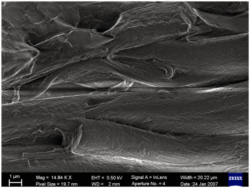
A SEM image of NLE. The average diameter of elastin fibers was determined to be 3–5 μm. In the image, it is clear that there are spaces between fibers, which accommodate component α2 proposed in Fig. 7.
The exchange between α1 ↔ β shows up later in time, and the exchange time is estimated to be longer than 100ms in the growth of the cross peak in the T2-T2 experimental data. The root mean square displacement, Δrrms, of water due to diffusion is given by
| (7) |
The time dependent diffusion coefficient of water in elastin fibers was measured previously by our group and is D = 8×10⁻⁶cm2/s for 1ms and D = 8×10⁻⁷cm2/s for 60ms at 10°C [25]. Therefore for a time of 1ms the displacement is approximately 2.1μm, and it is 5.4μm when t = 60ms, ignoring the tortuosity of the inner fiber morphology. The average diameter of elastin fibers, referring to Fig. 8, was measured to be 3–5μm. Thus, according to the computation, it takes more than 60ms for water inside fibers to diffusively exchange with water outside fibers and vice versa. This prediction is consistent with the experimental observation of a slow exchange rate between α1↔β, which again was greater than 100ms. The fast exchange rates for α1↔γ, α2↔γ, β↔γ observed in the experiments can also be explained by the model wherein γ on the surface is in close proximity to α1 and α2 and is also buried within the fiber and fast exchanges with β.
Given that a component of γ resides within the complex folding of the protein backbone and fast exchanges with α1, α2 or β it follows that the exchange of γ with other components can be considered separately. The component α1 fast exchanges with the γ molecules that are on the surface of the elastin fibers. Component α2, that is trapped within spaces between fibers, fast exchanges with γ on the surface of elastin fibers as well. Component β fast exchanges with γ inside the fiber morphology as well as α2 and α1. Therefore the complex, four-site (α1, α2, β and γ) system may be simplified into several two-site (e.g. α1 β, α2↔γ) systems. Thus, for each subsystem, an equation that involves only two sites may be implemented as follows:
| (8) |
In the above expression the subscripts i and j denote two distinguishable sites, based on their T2 times. The apparent relaxation times, accounting for exchange (i.e. K̄ ≠0), are given by
| (9) |
where denotes the long (+) and short (−) and relaxation rates [18]. The intensity of the cross peak is a function of and K̄ and may be written
| (10) |
where
| (11) |
| (12) |
| (13) |
| (14) |
Comparing the measured T1 values with the estimated exchange rates, it is evident that 1/T1 ≪ k for all compartments. Under this condition, Eq.9 simplifies to
| (15) |
and
| (16) |
Eq.10 may be written as
| (17) |
where
| (18) |
and
| (19) |
C1 and C2 are constants for a certain K̄ and .
In Eq.17 is the exchange time for waters exchanging between site i and j. This result is similar to that implemented by Washburn and Callaghan [15]. Eq.17 is fitted to the experimentally measured build up of cross peak intensity as a function of mixing time, where an exchange time is the best fit parameter for . To be clear, we fitted the parameters C1, C2 and to the experimental data. Two examples of cross peak growth curves between α1 ↔ γ and α2 ↔ γ on NLE at 25°C are shown in Fig.9. In the figure, the open points are experimental data, and the solid lines are the best fit curves to Eq.17. The only difference between the two curves is that the constant C1 is similar to C2 in Eq.17 for the open circles, while C1 is larger than C2 for the open squares in the fitting. The exchange time extracted for the open circles is and for the open squares. This measurement is consistent with the estimate on exchange times made earlier. It should be noted that the curves ultimately decay at longer mixing times due to T1 relaxation and are not shown in Fig.9. By fitting Eq.17 to all the cross peak intensities, the exchange times between different compartments were determined and are tabulated in Table 2. It is evident from the Table that the and exchange times are similar for water in both the NLE and the AE; this observation indicates that water molecules experience similar dynamics in both samples.
Fig. 9.

Two typical cross-peak growth curves determined by the mixing time dependence in the T2-T2 experiments. The open points are the experimental data from NLE at 25°C and the solid lines are the fitted curves to Eq.17. The error bars of the experimental data are within 5 percent of the number shown.
Table 2.
Measured exchange times [ ] (the inverse of the exchange rate) of D2O in bovine Nuchal Ligament Elastin (NLE) and bovine Aortic Elastin (AE), determined by fitting Eq.17 to the cross peak build up curves in the T2-T2 exchange experiments. The uncertainties are within 5 percent for all the data.
| Exchange times (ms) | NLE, 10°C | NLE, 25°C | NLE, 37°C | AE, 25°C | |
|---|---|---|---|---|---|
|
|
6.0 | 4.8 | 4.9 | 4.2 | |
|
|
6.6 | 3.5 | 5.1 | 2.7 | |
|
|
3.4 | 1.7 | 2.4 | 1.8 | |
|
|
5.4 | 1.7 | 3.3 | 5.5 | |
|
|
770 | 650 | 910 | 420 | |
It is well known that elastin undergoes an inverse temperature transition at approximately 15 to 25°C [1]. During the inverse temperature transition, elastin goes from a soluble state to an insoluble state with increasing temperature. Microscopically, hydrophobic association of β turns occur during the phase transition, and as a consequence, elastin’s volume decreases macroscopically with increasing temperature. In Urry’s description, water molecules that were originally in close proximity to the protein are pushed out and become more mobile free water. Experimentally, we find that the exchange rates of all the components appear to increase from 10 to 25°C. This observation appears to be consistent with the reduction in volume of the elastin fiber over this temperature range. Moreover, referring to Table 3, the intensity of the diagonal peak for γ at tm = 0.5 ms is observed to decrease upon increasing the temperature when going from 10C to 37°C. This observation indicates that the number of γ molecules decreases upon heating, which reveals that the γ component is indeed water that is in close proximity to the protein. We observed that the intensity of the α1 and α2 components increases from 10 to 37°C, which we attribute to water that has been squeezed out of the fibers as they are shrunk upon heating. The observation that the intensity of the γ component decreases with increasing temperature is also consistent with previous findings of our laboratory using deuterium Double Quantum Filtered (DQF) NMR [26]. The DQF NMR experiment allows one to probe the degree of anisotropic motion of nuclear spins, by monitoring the growth and subsequent decay of double quantum coherence created by a partially averaged quadrupolar interaction and well defined RF pulse sequence. In that work, the highly bound deuterium water molecules were observed to reduce in number at around 10 to 25°C, concomitant with a jump in the residual quadrupolar interaction (ωQ) at 10°C. The observed jump in ωQ appeared to be well correlated to the inverse temperature transition of elastin. When we raised the temperature further past 10°C to 37°C we observed a subsequent decrease in ωQ, indicative of a decrease in motional anisotropy of the γ component. Considering elastin and all waters of hydration as a closed thermodynamic system, the net entropy of all waters should increase upon increasing the temperature in order to obey the second law of thermodynamics. This is true because the local ordering of the protein increases during the phase transition, thereby decreasing its entropy. Referring to Table 1, we observed an increase in the T1 of all the components. The components α1, α2, and β all have relatively long T2 times and are thus in the fast-motion regime (i.e. τc ≫ ωo, where τc is the correlation time and ωo is the Larmor precession frequency). In this limit, the spin-lattice relaxation time is inversely proportional to the correlation time of motion, [27]. The observed increase in the T1 of all components with increasing temperature reveals a decrease in correlation time, indicative of an increase in motion and entropy. Lastly, referring to Table 2, the exchange times for all components decrease when the temperature is raised from 10 to 25°C. This observation is consistent with the decrease in the of all components from 10 to 25°C shown in Table 1, as the observed times are dependent on the exchange rates and the relaxation rates of other compartments according to Eq.9.
Table 3.
For NLE, the fractional contribution of the four components to the total signal at the different temperatures studied. It is observed that the abundance of α1 and α2 increase from 10 to 37°C, while the γ component and β component decrease from 25 to 37°C. This change appears to be well correlated to the negative thermal expansion coefficient of elastin over this temperature range. The numbers shown in the table were determined at a mixing time of 0.5 ms.
| NLE, 10°C | NLE, 25°C | NLE, 37°C | |
|---|---|---|---|
| α1 | 0.352 | 0.353 | 0.368 |
| α2 | 0.321 | 0.324 | 0.330 |
| β | 0.198 | 0.204 | 0.197 |
| γ | 0.129 | 0.120 | 0.105 |
4 Conclusion
In this work, we investigated the exchange of water in hydrated elastin by using 2D T1-T2 and T2-T2 correlation experiments. We studied the exchange of water in bovine nuchal ligament elastin and aortic elastin. We investigated the temperature dependence of the exchange rate of water in nuchal ligament elastin. The experimental data indicates that there are four exchanging sites. A model is proposed that quantifies the exchange between the sites by assuming that they exchange independently. The dynamics of water in nuchal ligament elastin and aortic elastin appear to be similar, indicating that the structural morphology may be identical. The temperature dependence of exchange rates indicates an increase of entropy in water at around 25°C where elastin undergoes the inverse temperature transition.
Acknowledgments
The authors thank Yi-Qiao Song of Schlumberger-Doll Research for allowing us to implement the ILT algorithm, Kathryn E. Washburn for fruitful discussions and Doug Wei for assisting us with SEM. G. S. Boutis acknowledges support from the Professional Staff Congress of the City University of New York and NIH grant number 7SC1GM086268-02. The content is solely the responsibility of the authors and does not necessarily represent the official views of the National Institute of General Medical Sciences or the National Institutes of Health.
References
- 1.Urry DW, Parker TM. J Muscle Research and Cell Motility. 2002;23:543–559. [PubMed] [Google Scholar]
- 2.Lillie MA, Gosline JM. Int J Biol Macromol. 2002;30:119–127. doi: 10.1016/s0141-8130(02)00008-9. [DOI] [PubMed] [Google Scholar]
- 3.Lillie MA, Gosline JM. Biopolymers. 1995;39:641–652. doi: 10.1002/(sici)1097-0282(199611)39:5<641::aid-bip3>3.0.co;2-w. [DOI] [PubMed] [Google Scholar]
- 4.Lillie MA, Gosline JM. Biopolymers. 1990;29:1147–1160. doi: 10.1002/bip.360290805. [DOI] [PubMed] [Google Scholar]
- 5.Mistrali F, Volpin D, Garibaldo GB, Ciferri A. J Phys Chem. 1971;75:142–150. doi: 10.1021/j100671a023. [DOI] [PubMed] [Google Scholar]
- 6.Kakivaya SR, Hoeve CAJ. Proc Nat Acd Sci. 1975;72:3505–3507. doi: 10.1073/pnas.72.9.3505. [DOI] [PMC free article] [PubMed] [Google Scholar]
- 7.Hoeve CAJ, Flory PJ. J Am Chem Soc. 1958;80:6523–6526. [Google Scholar]
- 8.Hoeve CAJ, Flory PJ. Biopolymers. 1974;13:677–686. doi: 10.1002/bip.1974.360130404. [DOI] [PubMed] [Google Scholar]
- 9.Li B, Alonso DOV, Bennion BJ, Daggett V. J Am Chem Soc. 2001;123:11991–11998. doi: 10.1021/ja010363e. [DOI] [PubMed] [Google Scholar]
- 10.Li B, Alonso DOV, Daggett V. J Mol Biol. 2001;305:581–592. doi: 10.1006/jmbi.2000.4306. [DOI] [PubMed] [Google Scholar]
- 11.Urry DW, Haynes B, Harris RD. Biochem Biophys Res Commun. 1986;141:749–755. doi: 10.1016/s0006-291x(86)80236-4. [DOI] [PubMed] [Google Scholar]
- 12.Urry DW. J Protein Chem. 1988;7:1–34. doi: 10.1007/BF01025411. [DOI] [PubMed] [Google Scholar]
- 13.Luan CH, Parker TM, Prasad KU, Urry DW. Biopolymers. 1991;31:465–475. doi: 10.1002/bip.360310502. [DOI] [PubMed] [Google Scholar]
- 14.Peemoeller H, Shenoy RK, Pintar MM. J Magn Reson. 1981;45:193–204. [Google Scholar]
- 15.Washburn KE, Callaghan PT. Phys Rev Lett. 2006;97:175502. doi: 10.1103/PhysRevLett.97.175502. [DOI] [PubMed] [Google Scholar]
- 16.Song YQ, Venkataramanan L, Hurlimann MD, Flaum M, Frulla P, Straley C. J Magn Reson. 2002;154:261–268. doi: 10.1006/jmre.2001.2474. [DOI] [PubMed] [Google Scholar]
- 17.Mitchell J, Griffith JD, Collins JHP, Sederman AJ, Gladden LF, Johns ML. J Chem Phys. 2007;127:234701. doi: 10.1063/1.2806178. [DOI] [PubMed] [Google Scholar]
- 18.Monteilhet J, Korb JP, Mitchell J, McDonald PJ. Phys Rev E. 2006;74:061404. doi: 10.1103/PhysRevE.74.061404. [DOI] [PubMed] [Google Scholar]
- 19.Van Landeghem M, Haber A, Lacaillerie JDD, Blumich B. Concepts in Magn Reson Part A. 2010;36A(3):153–169. [Google Scholar]
- 20.Partridge SM, Davies HF, Adair GS. Biochem J. 1955;61:11–21. doi: 10.1042/bj0610011. [DOI] [PMC free article] [PubMed] [Google Scholar]
- 21.Meiboom S, Gill D. Rev Sci Instrum. 1985;29:668. [Google Scholar]
- 22.Brownstein KR, Tarr CE. Phys Rev A. 1979;19:2446–2453. [Google Scholar]
- 23.Ellis GE, Packer KJ. Biopolymers. 1976;15:813–832. doi: 10.1002/bip.1976.360150502. [DOI] [PubMed] [Google Scholar]
- 24.Ellis GE, Packer KJ. Adv Exp Med Biol. 1977;79:663–678. doi: 10.1007/978-1-4684-9093-0_57. [DOI] [PubMed] [Google Scholar]
- 25.Boutis GS, Renner C, Isahkarov T, Islam T, Kannangara L, Kaur P, Mananga E, Ntekim A, Rumala Y, Wei D. Biopolymers. 2007;87:352–359. doi: 10.1002/bip.20838. [DOI] [PubMed] [Google Scholar]
- 26.Sun C, Boutis GS. J Magn Reson. 2010;205:86–92. doi: 10.1016/j.jmr.2010.04.007. [DOI] [PMC free article] [PubMed] [Google Scholar]
- 27.Abragam A. Principles of Nuclear Magnetism. Oxford University Press; 1983. pp. 313–315. [Google Scholar]