AUTOMATED ESTIMATION OF MICROTUBULE MODEL PARAMETERS FROM 3-D LIVE CELL MICROSCOPY IMAGES

Abstract

While basic principles of microtubule organization are well understood, much remains to be learned about the extent and significance of variation in that organization among cell types and conditions. Large numbers of images of microtubule distributions for many cell types can be readily obtained by high throughput fluorescence microscopy but direct estimation of the parameters underlying the organization is problematic because it is difficult to resolve individual microtubules present at the microtubule-organizing center or at regions of high crossover. Previously, we developed an indirect, generative model-based approach that can estimate such spatial distribution parameters as the number and mean length of microtubules. In order to validate this approach, we have applied it to 3D images of NIH 3T3 cells expressing fluorescently-tagged tubulin in the presence and absence of the microtubule depolymerizing drug nocodazole. We describe here the first application of our inverse modeling approach to live cell images and demonstrate that it yields estimates consistent with expectations.

1. INTRODUCTION

Microtubules play a critical role in many cellular processes and are a target of drugs used to treat cancer. The spatial distributions of microtubules are such that the density is very high close the centrosomal region and often very low at the lamellipodial region of the cell. High throughput image acquisition methods such as fluorescence microscopy can acquire images of an intact microtubule network, but their current resolution is not high enough to trace all individual microtubules in intact cells.

Currently, methods and validation sets have been generated on portions of microtubules that are clearly distinguishable, accounting for only a small fraction of the total microtubules in an intact cell [1, 2]. While these likely suffice for studying dynamics of microtubules that reach the lamellipodium, they do not allow construction of whole cell models.

We have previously described a generative model of microtubules and developed an indirect method of estimating its parameters [3]. Since whole cell images with known parameters were not available, we tested the ability of the method to accurately estimate model parameters using synthetic images generated using the model. These tests revealed a low error in estimation but estimates for real images could only be described as generally consistent with current knowledge. Here we describe estimation of microtubule model parameters from 3D fluorescence microscopy images of live cells under conditions in which changes in those parameters are expected. This was done by acquiring images of living NIH 3T3 cells expressing fluorescently-tagged tubulin in the presence and absence of nocodazole, a drug that is known to depolymerize microtubules [4].

2. DATA ACQUISITION

2.1. 3d NIH 3T3 dataset

NIH 3T3 cells expressing EGFP-tagged alpha tubulin generated using CD-tagging [5] were cultured in DMEM supplemented with 10% Fetal Calf Serum and 100 U/ml penicillin and 100 ug/ml streptomycin. The cells were grown to 80% confluency. On the day of imaging, the media was changed to Opti-MEM and a final concentration of 0.5 ug/ml of Hoechst was added to label nuclei. The dish was incubated for at least 3 h in a CO2 incubator and then placed in a heated chamber that was maintained at 37 °C throughout image acquisition. 3D images were acquired using a Zeiss LSM 510 confocal fluorescence microscope. The spacing between voxels was 0.09 microns in the focal plane and 0.48 microns along the axial dimension. 3D images of five different cells were acquired at 0, 10, 20, 30, 40 min after addition of nocodozale or buffer. Due to photobleaching, full 3D images could not be acquired for the same cell at each time point, and therefore different cells were imaged at each time point (only interphase cells were selected).

2.2. Fluorescent bead acquisition

As our modeling approach requires a model of the point spread function of the microscope used for acquisition, we generated an empirical estimate of the function using 20 nm fluorescent beads (488 nm absorption). 0.1 ml of a suspension of beads in optiMEM was placed on a clean glass slide and quickly covered by a coverslip. 3D images were acquired as above.

3. METHODS

3.1. Generative model of microtubules

The generative model of polymerized tubulin distribution previously described for HeLa cells [3] was applied to NIH 3T3 with only minor modifications. While the plasma membrane position for HeLa images was estimated using a fluorescence channel showing total cell protein, this channel was not available in the 3T3 images. The tubulin image itself was therefore used for this purpose since the presence of free tubulin allowed for a reliable estimate of cell boundaries.

3.2. Point spread function

3D images of beads were segmented into individual bead regions using Ridler-Calvard thresholding and registered using the 3D centroid of the bead. The beads were then averaged to estimate the point spread function.

3.3. Free tubulin distribution estimation and generation

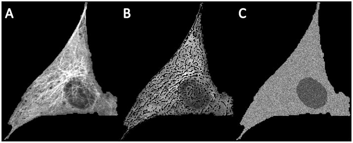
Our previous generative model only took into account polymerized tubulin because the images were acquired by immunofluorescence staining of fixed cells lacking appreciable free tubulin. This is because permeabilization of cells with detergents like Triton-X to allow antibody penetration causes most of the free tubulin to diffuse away. However, live cell imaging of fluorescently-tagged tubulin detects both free tubulin monomers and polymerized microtubules. We therefore extend the previous model to account for free tubulin by estimating histograms of free tubulin intensities h(reg, nz) for each nuclear or cytoplasmic region and for each 2D slice number nz. Free tubulin regions in each of the 2D slices was estimated by first detecting and removing the polymerized tubulin regions, as follows. The input image was blurred using a Gaussian filter with standard deviation of 3, and the resulting image was subtracted from the input image. The subtracted image was binarized to separate zero and nonzero pixels. Since the binary image has small clusters of disconnected objects seemingly forming microtubule fibers, the binary image is blurred again to connect objects that are close to each other. This operation was performed using a Gaussian filter with standard deviation of 2. The resulting image was again binarized. This ad hoc approach resulted in a reasonable definition of microtubules (as shown in Fig. 1). In order to generate free tubulin images for simulations, the histograms h(reg, nz) were sampled to generate the corresponding distribution of free tubulin in all regions of the cell, f(x).

Fig. 1.

(A) 2D slice from a 3D image stack of a cell untreated with nocodazole. (B) Removal of polymerized tubulin (C) Regeneration of free tubulin distribution by sampling from free tubulin intensity histograms estimated from (B).

3.4. Tubulin Image Formation

Here we describe the tubulin fluorescence image formation used for generating simulated images. Let I(x) be the tubulin fluorescence image. Let p(x) and f(x) be the polymerized tubulin and free tubulin images respectively. Let * denote a 3D convolution. Then, I(x) = psf *[p(x) + f(x)], where psf is the point spread function of the imaging system (estimated as above). This can be written as:

$$\begin{array}{c}I(x)=[\mathit{psf}\ast p(x)]+[\mathit{psf}\ast f(x)]\\ \mathit{psf}\ast p(x)=\mathit{psf}\ast [\lambda p^{\prime }(x)]=\lambda [\mathit{psf}\ast p^{\prime }(x)]\end{array}$$ (1)

where p′(x) is the model generated in pixel coordinates by the generative model for a given set of parameters and λ is the scaling factor that matches the single polymerized tubulin intensities in the simulated images to the real images (see below). Let f₂( x) = psf * f(x). Equation (1) then becomes:

$$I(x)=\lambda [\mathit{psf}\ast p^{\prime }(x)]+f_2(x).$$

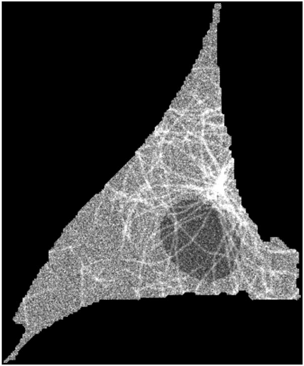
Hence, for a given set of parameters θ, I(x|θ) can be generated. For a given set of parameters, the amount of free tubulin was adjusted by scaling f₂ (x) according to the total amounts (total intensity) available (see Figure 2 for an example).

Fig. 2.

A 2D slice in the 3D stack of a simulated image. The image was generated with the number of microtubules set to 100, the mean of the length distribution to 60 microns, the standard deviation of length to 6 microns and the collinearity to 0.9961.

3.5 Single microtubule intensity estimation

The intensity of a single microtubule was estimated from the 2D slice and region just below the nucleus of the cell. The reason for this is that the microtubules (if present) in this region have a very minimal overlap and are generally traceable. λ was defined as:

$$\lambda =\frac{\varphi [p_R(x)]}{\varphi [p_S(x)]}$$

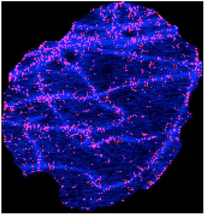
where ϕ[.] is the single microtubule intensity in the real (R) and simulated (S) images. ϕ[p_R(x)] was estimated by averaging tubular pixel values and subtracting out the average free tubulin pixel values. The tubular pixel regions were detected using the method described by Frangi et al. [6] (see Figure 3 for an example). The remaining regions were assumed to be free tubulin. ϕ[p_S(x)] was estimated directly from generated polymerized tubulin images p(x). λ was estimated from many images across the dataset and a single average value λ̄ was used.

Fig. 3.

Single microtubule intensity detection on microtubules in a slice just below the nucleus. The tubulin image is shown in blue and the points identified as showing a single microtubule are marked in red.

3.6 Library generation

As described in [3], a library of simulated images was generated for all combinations of discrete values of the four parameters:

• Number of microtubules = 0, 5, 20, 40, 60, 80, 100, 120, 140, 160, 180, 200, 220

• Mean of length distribution (μ) = 5, 20, 40, 60, 80, 100, 120, 140, 160, 180, 200, 220 microns

• Coefficient of variation of length = 0, 0.1, 0.2, 0.3

• Collinearity (cos α) = 0.97, 0.984, 0.992, 0.996, 1

3.7 Feature selection and matching

As described previously [3], parameters are indirectly estimated by choosing the synthetic image from the library that is most similar to a given real image. This choice is made using numerical features calculated to describe the fluorescence distributions, and a critical component of this approach is the choice of features and distance function. We describe here a feature selection method to include in the distance function using training data. Cells corresponding to the 40-min time point do not appear to have polymerized tubulin. Therefore features were selected so as to minimize the normalized Euclidean distance in feature space between 4 images of the 40-min time point of nocodazole treated cells and simulated images for 0 microtubules (only free tubulin).

4. RESULTS

3D confocal microscopy images were acquired at five different time points in the presence and absence of nocodazole, keeping all imaging parameters fixed. Figure 4 shows an example set of such images for various times of treatment with nocodazole.

Fig. 4.

Example images of NIH 3T3 cells expressing EGFP-tagged alpha-tubulin at various time points after addition of 20 uM nocodazole (from left to right, 0, 10, 20, 30, and 40 min).

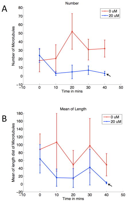
Cells treated with nocodazole for 40 min appear to have all of their microtubules depolymerized. All but one of the five images at this time point were therefore used to train the feature selection approach, and the features selected were used to estimate model parameters from all the images except the ones that were used for training. This procedure was repeated by holding out each image in turn (five-fold cross-validation). Figure 5 shows the parameter estimates averaged over the five folds and the five replicates per time point. Hence all points are averaged over 25 (5 folds × 5 replicates) except that the last time point is averaged over five folds only. The number and mean of length distribution for nocodazole-treated cells decrease as a function of time, but in the control case, these parameters do not show a decreasing trend. The standard deviation error bars are very large in some of the points. This is because the parameters are averaged over different cells that are likely to have varying numbers and lengths of microtubules because of their varying sizes. However, there is a clear decrease in the number and mean of the length from the first and last time points in the nocodazole treated case as opposed to the untreated case.

Fig. 5.

Parameter estimates of the number (A) and mean length (B) averaged over different folds and repetitions.

5. CONCLUSIONS AND DISCUSSION

We have validated a microtubule distribution estimation system by estimating parameters from an image set of live cells. The estimated parameters follow the expected trend: cells treated with nocodazole tend to have less polymerized tubulin. Future work will include improving many of the image processing routines to achieve higher efficiency and robustness, as well as exploring the dependence of the estimates on the accuracy of the point spread function.

In future, we plan to estimate parameters from different cell types. We also plan to build generative models of organelles (such as lysosomes or mitochondria) whose distribution may be conditioned on the microtubule model. Ultimately, we seek to build models in a hierarchical, conditional manner so that models of all cell components can be constructed by automated learning from cell images.

References

- 1.Gelasca ED, Byun J, Obara B, et al. Benchmark for evaluating biological image analysis tools. Workshop on Bio-Image Informatics: Biological Imaging, Computer Vision and Data Mining; Santa Barbara, CA: Center for Bio-Image Informatics, UCSB; 2008. [Google Scholar]
- 2.Sargin ME, Altinok A, Kiris E, et al. Tracing Microtubules in Live Cell Images. Proc. IEEE Int. Symp. Biomed. Imaging; 2007. pp. 296–299. [Google Scholar]
- 3.Shariff A, Murphy RF, Rohde GK. A generative model of microtubule distributions, and indirect estimation of its parameters from fluorescence microscopy images. Cytometry A. 2010 May;77(5):457–66. doi: 10.1002/cyto.a.20854. [DOI] [PMC free article] [PubMed] [Google Scholar]
- 4.Solomon F. Neuroblastoma cells recapitulate their detailed neurite morphologies after reversible microtubule disassembly. Cell. 1980 Sep;21(2):333–8. doi: 10.1016/0092-8674(80)90469-9. [DOI] [PubMed] [Google Scholar]
- 5.Jarvik JW, Fisher GW, Shi C, et al. In vivo functional proteomics: mammalian genome annotation using CD-tagging. Biotechniques. 2002 Oct;33(4):852–4. 856, 858–60. doi: 10.2144/02334rr02. passim. [DOI] [PubMed] [Google Scholar]
- 6.Frangi AF, Niessen WJ, Vincken KL, et al. Multiscale Vessel Enhancement Filtering. In: Wells W, Colchester A, Delp S, editors. Lecture Notes in Computer Science; Medical Image Computing and Computer-Assisted Interventation — MICCAI’98; Berlin/Heidelberg: Springer; 1998. [Google Scholar]