Comparing universal kriging and land-use regression for predicting concentrations of gaseous oxides of nitrogen (NOx) for the Multi-Ethnic Study of Atherosclerosis and Air Pollution (MESA Air)

Abstract

Background

Epidemiological studies that assess the health effects of long-term exposure to ambient air pollution are used to inform public policy. These studies rely on exposure models that use data collected from pollution monitoring sites to predict exposures at subject locations. Land use regression (LUR) and universal kriging (UK) have been suggested as potential prediction methods. We evaluate these approaches on a dataset including measurements from three seasons in Los Angeles, CA.

Methods

The measurements of gaseous oxides of nitrogen (NOx) used in this study are from a “snapshot” sampling campaign that is part of the Multi-Ethnic Study of Atherosclerosis and Air Pollution (MESA Air). The measurements in Los Angeles were collected during three two-week periods in the summer, autumn, and winter, each with about 150 sites. The design included clusters of monitors on either side of busy roads to capture near-field gradients of traffic-related pollution.

LUR and UK prediction models were created using geographic information system (GIS)-based covariates. Selection of covariates was based on 10-fold cross-validated (CV) R² and root mean square error (RMSE). Since UK requires specialized software, a computationally simpler two-step procedure was also employed to approximate fitting the UK model using readily available regression and GIS software.

Results

UK models consistently performed as well as or better than the analogous LUR models. The best CV R² values for season-specific UK models predicting log(NOx) were 0.75, 0.72, and 0.74 (CV RMSE 0.20, 0.17, and 0.15) for summer, autumn, and winter, respectively. The best CV R² values for season-specific LUR models predicting log(NOx) were 0.74, 0.60, and 0.67 (CV RMSE 0.20, 0.20, and 0.17). The two-stage approximation to UK also performed better than LUR and nearly as well as the full UK model with CV R² values 0.75, 0.70, and 0.70 (CV RMSE 0.20, 0.17, and 0.17) for summer, autumn, and winter, respectively.

Conclusion

High quality LUR and UK prediction models for NOx in Los Angeles were developed for the three seasons based on data collected for MESA Air. In our study, UK consistently outperformed LUR. Similarly, the 2-step approach was more effective than the LUR models, with performance equal to or slightly worse than UK.

1. Introduction

A central challenge in epidemiological analyses of the long-term impact of air pollution exposure on health is assigning exposures to individual subjects in cohort studies. Seminal studies in the field assigned exposures using area-wide monitored concentrations in different geographic regions (Dockery et al., 1993; Pope et al., 2002), but this approach ignores small-scale variation between individuals living within the same geographic region. More recent studies have incorporated intra-urban variation in ambient concentrations, with the exposures estimated by a variety of methods ranging from assigning the value measured at the nearest monitor to the subject’s home, to using distance to traffic as a proxy for traffic-related pollution, to predicting concentrations from complex spatial or spatio-temporal statistical models (Miller et al., 2007; Basu et al., 2000; Ritz et al., 2006; Puett et al., 2009; Adar et al., 2010).

Exposure studies have shown that levels of road traffic pollutants vary substantially within cities, often on the scale of meters (Briggs et al., 2000; Zhu et al., 2002; Gilbert et al., 2003). As such, studies have modeled intra-urban variation using multivariate regression based on Geographic Information System (GIS) covariates, often referred to as “land use” regression (LUR) (Briggs et al., 1997; Hoek et al., 2008; Brauer et al., 2003; Jerrett et al., 2005a; Su et al., 2009), and the geostatistical method kriging (Jerrett et al., 2005b; Künzli et al., 2005; Beelen et al., 2009). Little has been done, however, to explore the degree to which the predictive power of these models can be improved by combining predictions from LUR with smoothing of correlated residuals through universal kriging (UK).

The current study is motivated by the Multi-Ethnic Study of Atherosclerosis and Air Pollution (MESA Air), a prospective cohort study funded by the Environmental Protection Agency (EPA) to assess the associations between chronic exposure to air pollution and changes in sub-clinical markers of cardiovascular disease. Exposure assessment is based on existing regulatory monitoring networks as well as supplemental monitoring campaigns that include data collected at irregularly spaced times and locations (Cohen et al., 2009). Here we focus on spatial analysis of one of these supplementary monitoring campaigns, the “snapshot” campaign, which was designed to characterize spatial variability and roadway gradients using samples collected simultaneously at multiple locations across each city during three seasons. Ultimately, exposures for MESA Air will be predicted using a spatio-temporal model that incorporates all of the available monitoring data (Szpiro et al., 2010; Lindström et al., 2011; Sampson et al., 2011). The spatial analysis we present here provides insights into variable selection for the spatio-temporal model.

This paper focuses on evaluating spatial methods for predicting concentrations of gaseous oxides of nitrogen (NOx) from the MESA Air snapshot campaign in Los Angeles, CA. We compare the performance of LUR with UK, which can be viewed as a generalization of LUR that also incorporates kriging in order to exploit spatial correlation. We also consider a computationally simpler 2-step approximation to UK.

2. Methods

2.1. Study Design and Data

The Ogawa method was used to measure NOx concentrations (NO, NO₂, NOx, and SO₂ Sampling Protocol Using the Ogawa Sampler; Ogawa and Company, U.S.A., Inc.: Pompano Beach, FL, 1998). Concurrently deployed duplicate samples were used to assess precision. The mean relative percent difference for these samples in MESA Air was 5.2% with an RMSE of 6.1 ppb.

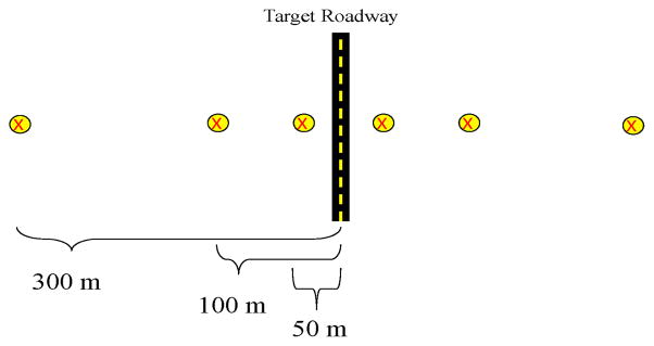
The snapshot campaign in downtown and coastal Los Angeles consists of 449 2-week average concentration measurements of NOx. These samples were collected during three 2-week periods in June 2006, October 2006, and January 2007. The sampling periods were chosen to capture seasonal differences and the sampling locations were chosen to maximize the variability of measured concentrations, characterize different land use categories, and cover the geographic region as broadly as possible. This campaign is described in greater detail by Cohen et al. (2009). In each round of monitoring, the majority of monitors were arranged in clusters of six, with three on either side of a major road at distances of approximately 50, 100, and 300 meters from the road. An example of an idealized roadway gradient cluster is shown in Figure 1.

Figure 1.

Idealized road gradient sampling scheme.

Over 300 GIS-based covariates were calculated for MESA Air. As described below, some were combined into composite covariates, and others were excluded because they did not have sufficient variability in the dataset. The approximately 65 covariates considered for model development are summarized in Table 1. All of the land use covariates were derived using the ArcGIS (Version 9.3, ESRI, Redlands, CA) software package based on land use data from the US Geological Survey (Price et al., 2006) roadway information from TeleAtlas Dynamap 2000(TeleAtlas ®, Lebanon, NH), and census data from the US Department of Commerce (2001). Census feature class codes (CFCC) were used to categorize roadways. The largest roads are designated as A1 (primary highways with limited access) while other major roads are designated as A2 (primary roads without limited access) or A3 (secondary and connecting roads). We derived an intense land use covariate that combines industrial, residential, transportation, commercial and services land use and an open space covariate that is the sum of bays, croplands and pastures, wetlands, forests, groves, rangeland, and sandy beach areas. These combined covariates were created for parsimony and because many of these land use and open space covariates did not have sufficient variability to be included in our models alone. The distance to coast variable is based on the Tele Atlas Dynamap 2000 County Boundary defined border of the Pacific Ocean.

Table 1.

GIS-based variables considered for model development. A1 roads are primary highways with limited access, A2 roads are primary roads without limited access, and A3 roads are secondary and connecting roads

Predictor Variable	Symbol	Units	Buffer radii	Functional Form
Non-roadway
Population	Pop	Total people within buffer (m)	500,1000,1500,2000, 2500,3000,5000, 10000,15000	scaled by 1/100,000
Intense Use Land	Int	km2	50, 100, 150, 300, 500 750, 1000, 1500, 2000, 3000	scaled by 1/100
Open Space Land	Open	km2	50, 100, 150, 300, 500 750, 1000, 1500, 2000, 3000	untransformed
Distance to Coast	D2C	meters	n/a	trunc. 15km & 25km scaled by 1/100,000
Distance to industrial Source (e.g., D2Comm: dist. to commercial, D2Lport: dist. to large port, D2Ryard: dist. to rail yard)	D2(variable)	meters	n/a
Roadway
Distance to nearest A1, A2, or A3	D2R	meters	n/a	Log101
Distance to nearest A1	D2A1	meters	n/a	Log101
Distance to nearest A2	D2A2	meters	n/a	Log101
Distance to nearest A3	D2A3	meters	n/a	Log101
Length of A1 roads within buffer	A1	meters	50, 100, 150, 300, 400, 500, 750, 1000, 5000 10000, 15000	scaled by 1/10,000
Length of A2 and A3 roads within buffer	A23	meters	50, 100, 150, 300, 400, 500, 750, 1000, 5000 10000, 15000	scaled by 1/100,000

¹Minimum distance of 10 meters.

2.2. Analysis

2.2.1. Land use regression and universal kriging

In this section we give a brief description of LUR and UK as well as an ad-hoc 2-step approximation to UK that can be easily fit using widely available software. We separately fit LUR and UK models to the log-transformed NOx concentration data from each of the three seasons. Log transformed NOx concentrations approximated a Normal distribution. Additional details of the LUR, UK, and the 2-step approach can be found in the Appendix.

LUR models are multiple linear regressions that assume independent residuals and use GIS-based covariates to predict concentrations at locations without measurements. UK can also be seen as a regression with geographic covariates but with the addition of correlated residuals. In other words, UK allows information about nearby concentration measurements to influence the predictions through the estimated correlation structure.

Kriging is a minimum mean-squared error approach to spatial prediction (Cressie, 1993; Banerjee et al., 2004). Unlike ordinary and simple kriging that assume an underlying constant mean surface, UK can be easily integrated with a regression model. The mean and covariance parameters for UK are estimated together using maximum likelihood through the geoR package in R (Ribeiro and Diggle, 2001). We assumed an exponential correlation structure.

ArcGIS is a widely available tool, but it does not allow UK with an arbitrary set of covariates or using maximum likelihood fitting. The ‘universal’ kriging option within ArcGIS models the spatial correlation as expected and allows the mean to be defined as a function of the latitude and longitude, but does not allow the use of land use covariates to be included in the mean model. The ‘simple’ and ‘ordinary’ krigings methods in ArcGIS model the spatial correlation and fit a constant mean. With these limitations in mind we also evaluated an ad-hoc 2-step approach to prediction, first estimating the LUR model assuming independent errors and then using simple kriging in ArcGIS to estimate the dependence in the LUR residuals and exploit this dependence to improve the predictions by smoothing. This approach, which is similar but not identical to UK, has some advantages: it allows for spatial structure in the residuals, whereas LUR does not, and it can be implemented with ArcGIS, whereas UK with land use covariates cannot. The 2-step procedure performs well in our examples, but we note that it may not be optimal because, unlike in UK, the regression coefficients are estimated without accounting for spatial correlation.

2.2.2. Cross-validation

The analysis in this paper employs a 10-fold cross-validation approach (Hastie et al., 2001). The exposure data are split into ten roughly equal size groups. To account for our unique study design, the clusters of six monitors were always kept within the same group. Then one group of data is set aside (test set) and the model is fit on the remaining nine groups (training set). The model estimated using the training set is used to predict values at the monitor locations in the test set. This is repeated until predictions for all groups have been generated. To evaluate the predictive ability of the model, R² and RMSE are calculated based on comparing these predicted values to the observations. We refer to these as the cross-validated (CV) R² and RMSE.

2.2.3. Model selection

Variable selection was done separately for each season and modeling approach (LUR or UK), all starting with the same set of covariates. We excluded covariates without at least 5% nonzero values in our data. Then the least absolute shrinkage and selection operator (lasso) was implemented as a prescreening tool via the glmnet function found in the R package glmnet (Friedman et al., 2010). The tuning parameter λ was selected to yield 15–20 nonzero regression coefficients from the lasso. We followed the lasso algorithm with a modified exhaustive search of the possible covariate combinations. The exhaustive search approach ensures that the model selection process accounts for the spatial correlation in the data, while the lasso algorithm does not account for this correlation. The final models were selected based on predictive ability as measured by cross-validated R² and RMSE.

In our exhaustive search, we considered no more than one buffer size for each covariate in any given model. In a recent paper, Su et al. (2009) reported on a methodology for selecting both a small- and long-range buffers for some geographic covariates. We restricted our models to a single (typically small) buffer size in the interest of parsimony and because coefficients for long-range buffer covariates are difficult to interpret in a model that predicts local concentrations.

In addition to the separate models for each season, a “common” model for all seasons was chosen via an exhaustive search of covariates that performed well in each of the seasons. When multiple models had the same cross validated R² and RMSE, the most parsimonious model was chosen.

3. Results

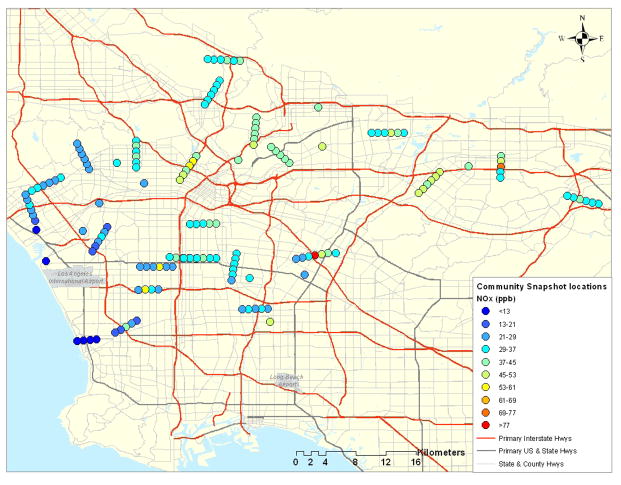
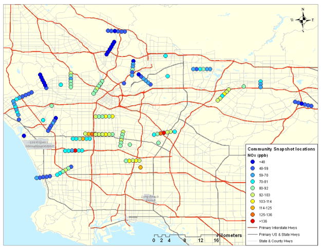
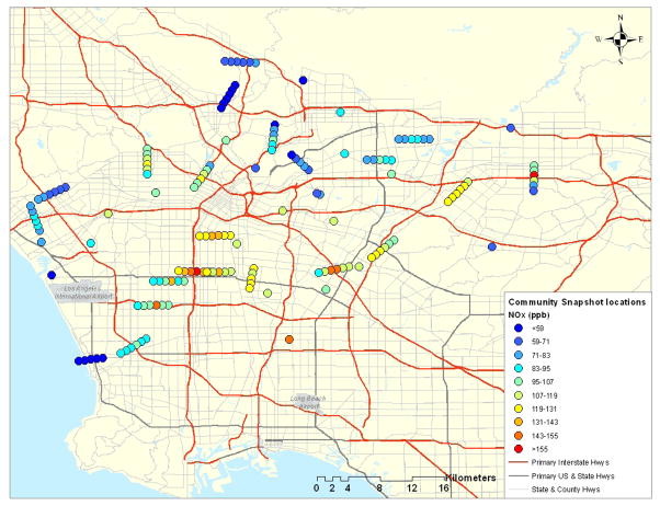
A total of 148, 152, and 149 monitoring locations were included in the analysis for summer, autumn, and winter, respectively. Sampling dates, cluster, and individual site allocations are summarized in Table 2a. Figures 2a, 2b, and 2c display the locations of the monitors in each season and their measured concentrations. Clustered data locations have been spread on the map for display purposes. Notably, there is evidence of a large-scale spatial gradient, with some of the lowest concentrations observed near the coast and higher values inland. We also see evidence of the roadway gradients, particularly inland where the highest concentrations in a given cluster are found at the monitors closest to the roads. In Table 2b we see that the magnitude of variability differs by season and the majority of the variability in NOx concentrations is between the individual sites and clusters as opposed to within clusters. Road clusters have similar means to individual sites. Except in summer, road cluster means are more variable than individual sites.

Table 2a.

Summary of Los Angeles NO_x snapshot monitoring locations

		Summer	Autumn	Winter
Dates	Start	6/27/2006	10/17/2006	1/23/2007
	End	7/12/2006	11/3/2006	2/7/2007
Samples	Total	148	152	149
	Clusters	24	24	23
	Individuals	14	13	20

Figure 2.

a Los Angeles sampling locations and concentrations in Summer 2006. The circles represent monitor locations. The distance between monitors and size of monitors have been exaggerated to make visualization of all locations possible.

b Los Angeles sampling locations and concentrations in Autumn 2006. The circles represent monitor locations. The distance between monitors and size of monitors have been exaggerated to make visualization of all locations possible.

c Los Angeles sampling locations and concentrations in Winter 2007. The circles represent monitor locations. The distance between monitors and size of monitors have been exaggerated to make visualization of all locations possible.

Table 2b.

Summary of Los Angeles NO_x snapshot concentrations (ppb)

		Summer	Autumn	Winter
All Sites	Mean	34.2	75.1	95.3
	Variance	132.1	551.0	728.4
Clusters	Mean	34.3	74.7	96.0
	Between Variance	89.6	450.5	620.4
	average w/in Variance	65.9	152.5	170.0
Individual Sites	Mean	31.2	77.7	91.0
	Between Variance	144.8	359.2	571.8

Results for models using variables selected based on LUR are shown in Table 3a. Using these variables, the LUR models explained 74%, 60%, and 67% of the variability with RMSE of 0.20, 0.20, and 0.17 in the summer, autumn, and winter, respectively. In all seasons UK and the 2-step approach had a cross validated R² greater than those of the LUR model (using variables selected for LUR). The distance to nearest A1 roadway and distance to coast covariates were present in the best models for all three seasons.

Table 3a.

Cross validated R² (RMSE) calculated for land use regression, universal kriging, and the 2-step approach for the ‘best’ model as chosen for predictive ability of land use regression in each season (on log(ppb) scale) for NOx

Season	Covariates	LUR	UK	2-step
Summer	D2A1, D2C, D2Comm, A23_50m, A1_50m, D2Lport, Int_3k	0.74 (0.20)	0.75 (0.19)	0.75 (0.19)
Autumn	D2A1, D2C, D2Comm, A23_50m, A1_50m, POP_5k	0.60 (0.20)	0.72 (0.17)	0.70 (0.17)
Winter	D2A1, D2C, A23_500m, D2R, Int_3k, D2Ryard	0.67 (0.17)	0.67 (0.17)	0.68 (0.17)

Results for models using variables selected based on UK are shown in Table 3b. The UK predictions explained 75%, 72%, and 74% of the variability with RMSE of 0.20, 0.17, and 0.15 in the summer, autumn, and winter, respectively. As with the variables selected based on LUR, we see that UK and the 2-step approach consistently outperform LUR in terms of prediction accuracy. Distances to nearest A1 roadway, coast, and commercial or service locations were included in the best model for each season.

Table 3b.

Cross validated R² (RMSE) calculated for land use regression, universal kriging, and the 2-step approach for the ‘best’ model as chosen for predictive ability of universal kriging in each season (on log(ppb) scale) for NOx

Season	Covariates	LUR	UK	2-step
Summer	D2A1, D2C, D2Comm, A23_50m	0.70 (0.21)	0.75 (0.20)	0.75 (0.20)
Autumn	D2A1, D2C, D2Comm, A23_50m, A1_50m, POP_5k	0.60 (0.20)	0.72 (0.17)	0.70 (0.17)
Winter	D2A1, D2C, D2Comm, A23_400m, A1_50m, Int_3k	0.48 (0.22)	0.74 (0.15)	0.70 (0.17)

The degradation in prediction accuracy for LUR models in winter in Table 3b compared with Table 3a is noteworthy. The difference is likely due to the fact that the winter LUR model selected based on UK fails to account for large scale spatial structure, while the corresponding model selected based on LUR includes additional covariates (D2R, D2Ryard) that have the potential to capture large-scale spatial structure.

We also identified a model that is common for all seasons. Here common is defined as having the highest average cross-validated R². The estimated coefficients and prediction performances for the common model are shown in Table 4. Overall the summer model is the most distinct, in part because large-scale spatial structure is captured in the mean model by the distance to coast covariate, resulting in a smaller estimated range. This may be related to the dominant on-shore wind in the Los Angeles region during the summer season. In the winter and autumn seasons, the wind is more variable so distance to coast is not as predictive of NOx concentrations, and we find a longer range for the residual spatial correlation.

Table 4.

Estimated parameters and standard errors for common model (on log(ppb) scale) for NOx. Details about the scaling of the covariates can be found in Table 1

Parameter	Summer	Autumn	Winter
Regression coefficient estimate (SE)
intercept	2.927 (0.25)	4.214 (0.25)	3.684 (0.25)
D2A1	−0.269 (0.04)	−0.161(0.04)	−0.137 (0.03)
A1_50m	−4.002 (7.02)	10.972 (5.37)	8.664 (4.26)
A23_400m	0.403 (0.28)	0.233 (0.22)	0.551 (0.19)
Pop_5k	−0.012 (0.03)	0.112 (0.03)	0.021 (0.03)
D2C	7.424 (0.69)	0.484 (0.92)	1.334 (1.03)
Int_3k	1.754 (0.77)	0.845 (0.76)	3.746 (0.88)
D2Comm	−1.507 (0.97)	−3.846 (0.80)	−2.071 (0.78)
Covariance
φ̂ (range in meters)	5,702	15,432	13,021
σ̂2 (partial sill)	0.030	0.016	0.027
τ̂2 (nugget)	0.011	0.023	0.010
Cross Validated R2(RMSE)
LUR	0.66 (0.22)	0.55 (0.19)	0.50 (0.21)
UK	0.70 (0.21)	0.68 (0.18)	0.72 (0.16)
2-step	0.70 (0.21)	0.66 (0.18)	0.70 (0.17)

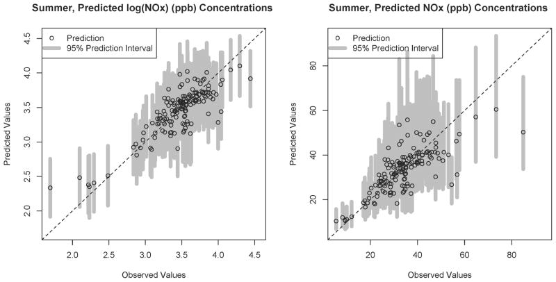
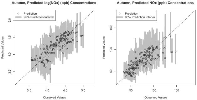
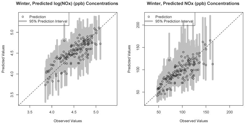
Figures 3a, 3b, and 3c show scatterplots of the observed and cross-validated predicted NOx concentrations (including 95% prediction intervals) at all of the monitoring locations in each of the three seasons, based on the common UK model. There are no notable outliers, and the prediction quality and interval coverage appear generally good, consistent with the R² values reported above.

Figure 3.

a Universal kriging predictions and 95% prediction intervals and observed concentrations in Summer 2006.

b Universal kriging predictions and 95% prediction intervals and observed concentrations in Autumn 2006.

c Universal kriging predictions and 95% prediction intervals and observed concentrations in Winter 2007.

The coefficient estimates vary across seasons, although mostly without changing sign. The two exceptions are A1 roads within 50 meters and population in a 5 km buffer; both these coefficients have negative signs in summer, although they also have very large standard errors. The common model consistently performed well in all seasons with cross-validated R² of 0.70, 0.68, and 0.72 (RMSE 0.21, 0.18, and 0.16) in the summer, autumn, and winter, respectively. As in the case of individual models for each season, UK and the 2-step approach have better predictive ability than LUR.

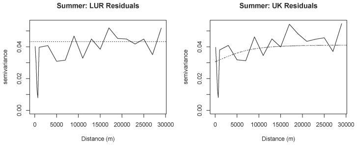
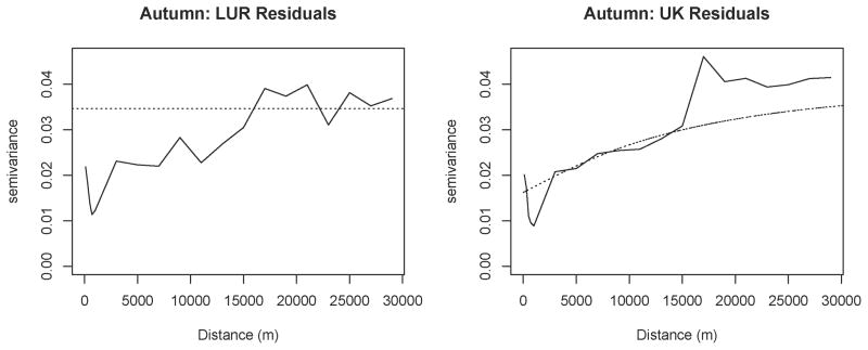
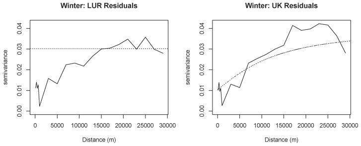
To further illustrate the advantages of UK, Figure 4a, 4b, and 4c show the variograms for the residuals in the summer, autumn, and winter season, respectively, from ordinary least squares regression models with covariates chosen in the common LUR and UK models. The residuals for both models clearly exhibit spatial structure. The initial drop in semivariance around 100 meters is likely due to a combination of wind direction coupled with our clustered design that is keenly sensitive to local traffic effects; Vienneau et al. (2010) observed a similar phenomenon in their LUR models. As an additional test for spatial correlation, we applied a Moran’s I test with inverse-distance weighting (Paradis et al., 2004). The Moran’s I test was statistically significant with p < 0:001 for all six sets of residuals. The LUR approach does not exploit the spatial correlation for predictions, instead assuming independent observations. UK estimates the covariance and incorporates the spatial structure in predictions; the result is improved predictive performance.

Figure 4.

a Display of the variograms for land use regression and universal kriging common model residuals for the summer season. The dotted black line is the covariance function estimated by the model for each approach.

b Display of the variograms for land use regression and universal kriging common model residuals for the autumn season. The dotted black line is the covariance function estimated by the model for each approach.

c Display of the variograms for land use regression and universal kriging common model residuals for the winter season. The dotted black line is the covariance function estimated by the model for each approach.

4. Discussion

Epidemiological studies of air pollution and health outcomes rely on quality predictions of air pollution concentrations at sites without monitoring data. The modeling approaches taken in this paper have proven to be effective at capturing small-scale variability, as measured by cross-validated R², and are reasonably straightforward to implement in readily available software (e.g. ArcGIS, R).

In our study, UK yielded cross-validated R² for log-transformed NOx concentrations ranging from 0.72–0.75. The best models selected for LUR were not as good but were still able to achieve reasonable predictive ability (CV R² ranged from 0.60–0.74). Previous LUR studies of oxides of nitrogen (NO, NO₂, or NOx) have yielded cross validated R² values ranging from 0.49–0.87 (Hoek et al., 2008).

A recent paper that analyzed NOx concentrations in Los Angeles reported an R² value of 0.92 based on LUR, but this number is estimated using a single test set of only 16 locations so it is difficult to assess its generalizability (Su et al., 2009). Other considerations such as the distribution of monitor locations and variability in measured concentration also impact R² and may explain the difference between our results and those reported by Su et al. (2009).

Previous studies have shown LUR performing better than ordinary kriging, which relies solely on spatial smoothing without incorporating covariates. Few studies have compared LUR and UK or entertained a 2-step approach along the lines of the one we describe. One exception is a recent paper that demonstrated the superiority of UK over other modeling approaches in mapping background air pollution across the European Union (Beelen et al., 2009). In our study, UK consistently outperformed LUR. Similarly, the 2-step approach was more effective than the LUR models, with performance equal to or slightly worse than UK. Even for the models selected for their LUR performance, the UK and 2-step approaches performed as well or better in all seasons.

Since air pollution emission and dispersion is a deterministic process, one might argue that the improved performance via correlated residuals masks the absence of important variables from our models. However, the inability to collect or precisely quantify all variables affecting pollution should be viewed as an inherent aspect of exposure assessment. Even with MESA Air’s highly detailed set of GIS variables, there remained substantial unaccounted-for spatial correlations. Hence, incorporating these correlations in the model is the preferred approach both practically and conceptually.

Our results indicate that the 2-step approach has predictive ability similar to UK. This is encouraging since it provides an additional option for researchers less familiar with using flexible tools to fit UK models (such as geoR). The 2-step approach is based on first fitting a mean model using standard linear regression and then modeling the spatial correlation between residuals using tools available in ArcGIS. This approach is preferable to choosing between ordinary kriging (assuming a constant mean) and land use regression (assuming independence).

The important model selection stage still needs to be performed separately. At present, there is no single optimal solution for model selection. However, it is important to choose an approach that works well for the research problem at hand, and appropriately handles highly correlated covariates (e.g. traffic density or population in different size buffers).

Validation is an essential part of assessing the performance and robustness of a model, and its design should be considered carefully. The results in this paper use 10-fold cross-validated R² (Hastie et al., 2001), with specific consideration given to the clustered design of our the monitoring data. Since we used cross-validation as part of the model selection procedure, our reported prediction accuracy may still be somewhat optimistic because the same data were used for selection and final evaluation. As an alternative to cross validation, some authors (e.g. Su et al. (2009)) consider a test data set that is separate from the training data. This has the virtue of providing independent test data, but if the test data set is relatively small (which it often must be in order to have sufficient training data available to fit the model) the resultant R² value can be less informative than the cross-validated R² about sensitivity of the model to possible extreme observations. Moreover, as is the case with cross validation, typically the test set’s locations are similar in nature to the training set, and not to the eventual target locations thus the estimated prediction accuracy may be biased.

There was considerable variability between seasons in the magnitude, and in some cases also the signs, for the common model coefficient estimates and spatial covariance model parameters shown in Table 4. In particular, summer has the shortest range, indicating the spatial correlation is the smallest in this season, while autumn and winter show evidence of longer range correlation. One possible explanation for this discrepancy is that the distance-to-coast covariate captures the effect of prevailing winds in summer and accounts for the dominant spatial structure in the data, whereas this simple covariate does not account for the more complex circulation patterns in autumn and winter. The variability between seasons suggests that it would be unwise to use our dataset to naively model all three seasons jointly or to combine them in a single model to predict long-term average concentrations. Instead, we incorporate our findings from analyzing the snapshot data into the MESA Air spatio-temporal model (Szpiro et al., 2010; Lindström et al., 2011) to reliably predict NOx concentrations at subject locations over several years and derive long-term average exposures for the time periods of interest based on these predictions.

Table 2c.

Summary of Los Angeles log(NO_x) snapshot concentrations (log(ppb))

		Summer	Autumn	Winter
All Sites	Mean	3.47	4.27	4.51
	Variance	0.15	0.10	0.09
Clusters	Mean	3.47	4.26	4.52
	Between Variance	0.14	0.09	0.08
	average w/in Variance	0.04	0.02	0.02
Individual Sites	Mean	3.35	4.32	4.48
	Between Variance	0.24	0.06	0.07

Research Highlights.

• Land use regression (LUR) and universal kriging (UK) predict NOx in Los Angeles

• UK with traffic, population, land use, and geographic covariates outperforms LUR

• Optimal model choice varies between three seasons

• Nearly-optimal model performs well in all three seasons

Abbreviations

UK

universal kriging

LUR

land use regression

CV

cross validated

RMSE

root mean square error

Appendix

Land use regression model

Take our monitoring data to be Y⃗ = (Y (s₁),…, Y (s_n))^T, where Y (s_i) is the observed concentration at location s_i. We also have a set of M (where M ≥ n) land use covariates to be used as predictors. We model the data as:

$$Y(s_i)={\beta }_0+\sum _{j=1}^k{\beta }_j{x}_{i,j}+{\epsilon }_i\text{where}{\epsilon }_i\sim N(0,{\nu }^2)\text{and}i=1,\dots n$$

equivalently,

$$\overrightarrow{Y}(s)=\mathbf{X}(s)\overrightarrow{\beta }+\overrightarrow{\epsilon }\text{where}\overrightarrow{\epsilon }\sim N(0,{\nu }^2)$$

where X(s) are the GIS-based covariates from sampled sites, respectively. Let s₀ indicate locations without concentration data (e.g. subject homes) and Y (s₀) be the corresponding unobserved concentration at location s₀. The estimated regression parameters $\overrightarrow{\widehat{\beta }}$ are used to predict NO_x concentrations at unmeasured location with:

$$E[\overrightarrow{Y}(s_0)\mid \overrightarrow{Y}(s);\mathbf{X}(s_0)]=\mathbf{X}(s_0)\overrightarrow{\widehat{\beta }}$$

Universal Kriging

Regression and covariance parameters are estimated by fitting the following model with the geoR package in R Ribeiro and Diggle (2001):

$$\overrightarrow{Y}(s)=\mathbf{X}\overrightarrow{\beta }+\overrightarrow{\epsilon }\text{with}\overrightarrow{\epsilon }\sim N_m(0,\mathrm{\sum }({\sigma }^2,{\tau }^2,\phi ))$$

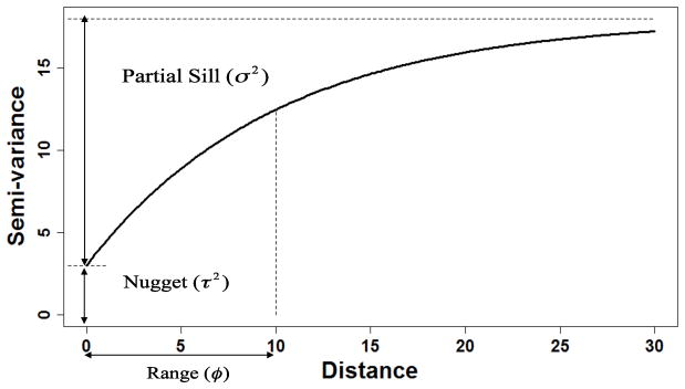
A covariance function must be specified. We use the exponential covariance model, which models the covariance of two measurements as a function of the distance between them such that

$$C(d)=\{\begin{array}{ll}{\sigma }^{2}exp(-d/\phi )\hfill & \text{if}d>0\hfill \\ {\tau }^2+{\sigma }^2\hfill & \text{if}d=0\hfill \end{array}$$

where d is the distance between observations. A theoretical variogram for the exponential correlation function is shown in Figure 5.

Figure 5.

Theoretical exponential variogram.

Assuming Y⃗ (s) and Y⃗ (s₀) are jointly normal, from standard multivariate normal theory we have the result:

$$\left(\begin{array}{c}\overrightarrow{Y}(s_0)\\ \overrightarrow{Y}(s)\end{array}\right)\sim N\left(\left(\begin{array}{c}\mathbf{X}(s_0)\overrightarrow{\beta }\\ \mathbf{X}(s)\overrightarrow{\beta }\end{array}\right),\left(\begin{array}{cc}{\mathrm{\sum }}_{11}& {\mathrm{\sum }}_{12}\\ {\mathrm{\sum }}_{21}& {\mathrm{\sum }}_{22}\end{array}\right)\right)$$

where ${\mathrm{\sum }}_{12}={\mathrm{\sum }}_{21}^T$ Predictions for unmeasured locations s₀ are generated using the conditional distribution of unobserved data given observed data at locations s:

$$E[\overrightarrow{Y}(s_0)\mid \overrightarrow{Y}(s)]\sim N(\mathbf{X}(s_0)\overrightarrow{\beta }+{\mathrm{\sum }}_{12}{\mathrm{\sum }}_{22}^{-1}(\overrightarrow{Y}(s)-\mathbf{X}(s)\overrightarrow{\beta }),{\mathrm{\sum }}_{11}-{\mathrm{\sum }}_{12}{\mathrm{\sum }}_{22}^{-1}{\mathrm{\sum }}_{21})$$

2 - step predictions with LUR & simple kriging

As in LUR the multivariate regression model Y⃗ (s) = X(s)β⃗ + ε⃗ is fit, where ε⃗ ~ N(0, ν²). Simple kriging is used with the regression residuals, ε⃗, to estimate Σ(σ², τ², φ). Then, as in universal kriging, predictions are based on the normal conditional expectation of Y⃗ (s₀) given Y⃗ (s). Operationally, this involves adding the land use regression predictors with the simple kriging prediction.

References

- Adar SD, Klein R, Klein BEK, Szpiro AA, Cotch MF, Wong TY, O’Neill MS, Shrager S, Barr RG, Siscovick D, Daviglus ML, Sampson PD, Kaufman JD. Air pollution and the human microvasculature in vivo assessed via retinal imaging: The Multi-Ethnic Study of Atherosclerosis and Air Pollution (MESA Air) PLOS Medicine. 2010;7(11) doi: 10.1371/journal.pmed.1000372. [DOI] [PMC free article] [PubMed] [Google Scholar]
- Banerjee S, Carlin BP, Gelfand AE. Hierarchical Modeling and Analysis for Spatial Data. Chapman and Hall; 2004. [Google Scholar]
- Basu R, Woodruff TJ, Parker JD, Saulnier L, Schoendorf KC. Particulate air pollution and mortality: Findings from 20 u.s. cities. New England Journal of Medicine. 2000;343 (24):1742–1749. doi: 10.1056/NEJM200012143432401. [DOI] [PubMed] [Google Scholar]
- Beelen R, Hoek G, Pebesma E, Vienneau D, de Hoogh K, Briggs DJ. Mapping of background air pollution at a fine spatial scale across the european union. Science of the Total Environment. 2009;407 (6):1852–1867. doi: 10.1016/j.scitotenv.2008.11.048. [DOI] [PubMed] [Google Scholar]
- Brauer M, Hoek G, van Vliet P, Meliefste K, Fischer P, Gehring U, Heinrich J, Cyrys J, Bellander T, Lewne M, Brunekreef B. Estimating long-term average particulate air pollution concentrations: application of traffic indicators and geographic information systems. Epidemiology. 2003;14 (2):228–239. doi: 10.1097/01.EDE.0000041910.49046.9B. [DOI] [PubMed] [Google Scholar]
- Briggs DJ, Collins S, Elliot P, Fischer P, Kingham S, Lebret E, Pryl K, Van Reeuwijk H, Smallbone K, Van der Veen A. Mapping urban air pollution using gis: a regression-based approach. International Journal of Geographical Information Science. 1997;11:699–718. [Google Scholar]
- Briggs DJ, de Hoogh C, Gulliver J, Wills J, Elliot P, Kingham S, Smallbone K. A regression-based method for mapping traffic-related air pollution: application and testing in four contrasting urban environments. Science of the Total Environment. 2000;253 (1–3):151–167. doi: 10.1016/s0048-9697(00)00429-0. [DOI] [PubMed] [Google Scholar]
- Cohen MA, Adar SD, Allen RW, Avol E, Curl CL, Gould T, Hardie D, Ho A, Kinney P, Larson TV, Sampson PD, Sheppard L, Stukovsky KD, Swan SS, Liu LJ, Kaufman JD. Approach to estimating participant pollutant exposures in the multi-ethnic study of atherosclerosis and air pollution (mesa air) Environmental Science and Technology. 2009 July;43 (13):4687–4693. doi: 10.1021/es8030837. [DOI] [PMC free article] [PubMed] [Google Scholar]
- Cressie NAC. Wiley series in probability and mathematical statistics. Wiley; 1993. Statistics for spatial data. [Google Scholar]
- Dockery DW, Pope CA, Xu X, Spangler JD, Ware JH, Fay ME, Ferris BG, Speizer FE. An association between air pollution and mortality in six cities. New England Journal of Medicine. 1993;329 (24):1753–1759. doi: 10.1056/NEJM199312093292401. [DOI] [PubMed] [Google Scholar]
- Friedman J, Hastie T, Tibshirani R. Regularization paths for generalized linear models via coordinate descent. Journal of Statistical Software. 2010;33 (1):1–22. [PMC free article] [PubMed] [Google Scholar]
- Gilbert NL, Woodhouse S, Stieb DM, Brook JR. Ambient nitrogen dioxide and distance from a major highway. Science of the Total Environment. 2003;312 (1–3):43–46. doi: 10.1016/S0048-9697(03)00228-6. [DOI] [PubMed] [Google Scholar]
- Hastie T, Tibshirani R, Friedman J. The Elements of Statistical Learning Data Mining, Inference, and Prediction. Springer; 2001. [Google Scholar]
- Hoek G, Beelen R, de Hoogh K, Gulliver J, Fischer P, Briggs DJ. A review of land-use regression models to assess spatial variation of outdoor air pollution. Atmospheric Environment. 2008;42:7561–7578. [Google Scholar]
- Jerrett M, Arain A, Kanaroglou P, Beckerman B, Potoglou D, Sahsu-varoglu T, Morrison J, Giovis C. A review and evaluation of in-traurban air pollution exposure models. Journal of Exposure Analysis and Environmental Epidemiology. 2005a;15:185–204. doi: 10.1038/sj.jea.7500388. [DOI] [PubMed] [Google Scholar]
- Jerrett M, Buzzelli M, Burnett RT, DeLuca PF. Particulate air pollution, social confounders, and mortality in small areas of an industrial city. Social Science and Medicine. 2005b;60 (12):2845–2863. doi: 10.1016/j.socscimed.2004.11.006. [DOI] [PubMed] [Google Scholar]
- Künzli N, Jerrett M, Mack WJ, Beckerman B, LaBree L, Gilliland F, Thomas D, Peters J, Hodis HN. Ambient air pollution and atherosclerosis in los angeles. Environmental Health Perspectives. 2005;113 (2):201–206. doi: 10.1289/ehp.7523. [DOI] [PMC free article] [PubMed] [Google Scholar]
- Lindström J, Szpiro A, Sampson P, Sheppard L, Oron A, Richards M, Larson T. A flexible spatio-temporal model for air pollution: Allowing for spatio-temporal covariates. UW Biostatistics Working Paper Series (Working Paper 370) 2011 [Google Scholar]
- Miller KA, Siscovick DS, Sheppard L, Shepherd K, Sullivan JH, Anderson GL, Kaufman JD. Long-term exposure to air pollution and incidence of cardiovascular events in women. New England Journal of Medicine. 2007;356:447–458. doi: 10.1056/NEJMoa054409. [DOI] [PubMed] [Google Scholar]
- Paradis E, Claude J, Strimmer K. APE: analyses of phylogenetics and evolution in R language. Bioinformatics. 2004;20:289–290. doi: 10.1093/bioinformatics/btg412. [DOI] [PubMed] [Google Scholar]
- Pope CA, Burnett RT, Thun MJ, Calle EE, Ito K, Krewski D, Thurston GD. Lung cancer, cardiopulmonary mortality, and long-term exposure to fine particulate air pollution. Journal of the American Medical Association. 2002;9 (287):1132–1141. doi: 10.1001/jama.287.9.1132. [DOI] [PMC free article] [PubMed] [Google Scholar]
- Price C, Nakagaki N, Hitt KJ, Clawges RC. Tech rep. U.S. Geological Survey Digital Data Series; 2006. Enhanced historical land-use and land-cover data sets of the u.s. geological survey; p. 240. URL http://pubs.usgs.gov/ds/2006/240. [Google Scholar]
- Puett RC, Hart JE, Yanosky JD, Paciorek C, Schwartz J, Suh H, Speizer FE, Laden F. Chronic fine and coarse particulate exposure, mortality, and coronary heart disease in the Nurses’ Health Study. Environmental Health Perspectives. 2009;117 (11):1697–1701. doi: 10.1289/ehp.0900572. [DOI] [PMC free article] [PubMed] [Google Scholar]
- Ribeiro PJ, Diggle PJ. geoR: a package for geostatistical analysis. R-NEWS. 2001;1 (2):14–18. [Google Scholar]
- Ritz B, Wilhelm M, Zhao Y. Air pollution and infant death in southern california, 1989–2000. Pediatrics. 2006;118 (2):493–502. doi: 10.1542/peds.2006-0027. [DOI] [PMC free article] [PubMed] [Google Scholar]
- Sampson PD, Szpiro AA, Sheppard L, Lindström J, Kaufman JD. Pragmatic estimation of a spatio-temporal air quality model with irregular monitoring data. Atmospheric Environment. 2011 In Press. [Google Scholar]
- Su JG, Jerrett M, Beckerman B, Wilhelm M, Ghosh JK, Ritz B. Predicting traffic-related air pollution in los angeles using a distance decay regression selection strategy. Environmental Research. 2009;109 (6):657–670. doi: 10.1016/j.envres.2009.06.001. [DOI] [PMC free article] [PubMed] [Google Scholar]
- Szpiro AA, Sampson PD, Sheppard L, Lumley T, Adar SD, Kaufman JD. Predicting intra-urban variation in air pollution concentrations with complex spatio-temporal dependencies. Environmetrics. 2010;21:606–631. doi: 10.1002/env.1014. [DOI] [PMC free article] [PubMed] [Google Scholar]
- US Department of Commerce, WD. Us census bureau, tiger/line files redistricting census 2000. 2001 URL http://www.census.gov/geo/www/tiger.
- Vienneau D, de Hoogh K, Beelen R, Fischer P, Hoek G, Briggs D. Comparison of land-use regression models between Great Britain and the Netherlands. Atmospheric Environment. 2010;44 (5):688–696. [Google Scholar]
- Zhu YF, Hinds WC, Kim S, Shen S, Sioutas C. Study of ultrafine particles near a major highway with heavy-duty diesel traffic. Atmospheric Environment. 2002;36 (27):4323–4335. [Google Scholar]