

Abstract
Background In a famous article, Simpson described a hypothetical data example that led to apparently paradoxical results.
Methods We make the causal structure of Simpson's example explicit.
Results We show how the paradox disappears when the statistical analysis is appropriately guided by subject-matter knowledge. We also review previous explanations of Simpson's paradox that attributed it to two distinct phenomena: confounding and non-collapsibility.
Conclusion Analytical errors may occur when the problem is stripped of its causal context and analyzed merely in statistical terms.
Keywords: Simpson's paradox, causal diagrams, confounding, collapsibility
Introduction
In 1951, E.H. Simpson1 published an article on the analysis of 2 × 2 tables. The last part of the article included a hypothetical example that involved three dichotomous variables, and that resulted in apparently surprising results. This hypothetical example inspired what was later referred to as Simpson's paradox,2 reversal paradox3 and amalgamation paradox.4 Here, we argue that the apparent paradox originally described by Simpson is the result of disregarding the causal structure of the research problem. In fact, any hint of a paradox disappears when the causal structure is made explicit. We also review previous explanations of Simpson's paradox that attributed it to two distinct phenomena—confounding and non-collapsibility. First, let us review Simpson's famous example.
Simpson's example
Simpson presented the following numerical example. Let A, B and C be three dichotomous variables measured in a population of N = 52 individuals. The data can be summarized via the following three 2 × 2 contingency tables:
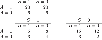
The odds ratio (OR) that measures the association between A and B is  in the first table, and
  in each of the two tables stratified by C. That is, even though the conditional odds ratio is the same within both levels of C, the conditional and marginal (unconditional) associations are not equal. We say that A and B are marginally (unconditionally) independent, A ∐ B, and that A and B are conditionally dependent given C,
  .
.
Which odds ratio is the most sensible measure of association between A and B? The marginal ORAB or the conditional ORAB|C? Simpson designed his example to show that the answer to this question depends on the research setting. He considered two sets of labels for variables A, B and C.
First, suppose that ‘An investigator wished to examine whether in a pack of [52] cards the proportion of court cards (King, Queen, Knave) was associated with colour (Red, Black). It happened that the pack which he examined was one with which Baby had been playing, and some of the cards were dirty.’ Let A be the type of card (1: plain, 0: court), B the card's colour (1: black, 0: red) and C whether the card was dirty (1: yes, 0: no). In this setting, the investigator would be interested in the marginal odds ratio ORAB, which is obviously 1 as a cards deck contains the same number of black and red court cards.
Secondly, suppose that A represents some medical treatment (1: yes, 0: no), B represents death (1: yes, 0: no) and C represents chromosomic sex (1: male, 0: female). In this setting, the investigator would be interested in the conditional odds ratio ORAB|C, which shows that the treatment is associated with a lower risk of death in both men and women.
Hence, the apparent paradox to which Simpson drew attention: even if the conditional A–B association measure is homogeneous within levels of C, the sensible answer is sometimes the conditional association measure and other times the marginal one. From a purely statistical standpoint, no general rule seems to exist as to whether the conditional association or the marginal association should be preferred.
A causal interpretation of Simpson's example
The causal diagram in Figure 1 depicts the variables court card (A), card colour (B) and dirty card (C). There is no arrow between A and B because card type and colour do not cause each other. There is an arrow from A to C because, according to the example above, the baby had a strong predilection for court cards (ORAC = 0.34). Similarly, there is an arrow from B to C because the baby preferred the red cards (ORBC = 0.52).
Figure 1.

A collider C
The common effect C in Figure 1 is referred to as a collider because two arrowheads collide into it. Graph theory shows that conditioning on a collider C generally introduces an association between its causes A and B even if the causes are marginally independent.5,6 Therefore, the association that appears between A and B only when the analysis is conditional on C is not surprising but expected. Informally, if we select a court card that is known to be dirty, then it is less likely that the card is red. In fact, the only surprising fact is that the baby managed to get cards dirty in such a way that the odds ratio ORAB|C=1 among the dirty was exactly equal to the odds ratio ORAB|C=0 among the clean. The baby was either mathematically gifted or quite lucky. The association created between two variables by conditioning on, or selecting a stratum of, their common effect is often referred to as selection bias by epidemiologists.7 Epidemiological examples with the same structure as Figure 1 are ubiquitous. For example, when estimating the effect of genetic factor A on diabetes B, one would generally introduce selection bias by conditioning on the history of heart disease C.
The causal diagram in Figure 2 depicts the variables treatment (A), death (B) and sex (C). There is an arrow from C to A because men were less likely to receive treatment (ORAC = 0.34), which implies that treatment A was not randomly assigned in the study population. Similarly, there is an arrow from C to B because men were less likely to die (ORBC = 0.52). The arrow from A to B represents the direct effect that is responsible for the conditional association observed between treatment and death within the levels of sex.
Figure 2.

A confounder C
Graph theory5,6 shows that a common cause like C will create an association between its effects A and B. This association does not reflect the causal effect of A on B and is commonly referred to as confounding. Conditioning on variable C removes the confounding (i.e. the assignment of treatment A is ignorable given C8). We say that a variable is a confounder when it can help eliminate confounding,9 so C is a confounder in Figure 2 but not in Figure 1. In Simpson's example, the confounding results in a positive (OR > 1) association between A and B because men are less likely to be treated and also less likely to die.10 Thus, there are two sources of association between treatment A and death B: the positive association due to confounding by C and the negative association presumably due to the protective effect of treatment A on the risk of death B. The marginal odds ratio (ORAB = 1) measures the combination of these two associations. Again, the only surprising aspect of these data is that both sources of association, each in one direction, cancel out each other exactly and result in marginal independence. In general, one would expect that the marginal odds ratio would be different from 1: ORAB > 1 if the association due to confounding is greater than the association due to the effect of treatment on death, and ORAB < 1 otherwise.
The above discussion of Simpson's example relies on a crucial fact: the direction of the causal arrows in Figures 1 and 2 is determined by the causal structure of the problem, not by statistical considerations. In Figure 1, card type and colour affect the risk of the card being dirty, but getting the card dirty does not affect its type and colour. In Figure 2, sex may affect death or treatment, but death or treatment cannot affect sex. The data and the odds ratios, however, look exactly the same in both cases. Thus, a treatment of Simpson's example that ignores the causal structure does not contain sufficient information to determine the appropriateness of the marginal vs the conditional association measure.
On the other hand, a data analyst with enough expert knowledge will correctly identify the causal structure of the problem, and therefore will make the correct decision. Under Figure 1, one will use the marginal association to prevent selection bias. Under Figure 2, one will use the conditional association to eliminate confounding. So there is a general recommendation—albeit not a purely statistical one because it requires correct expert knowledge—for 2 × 2 tables after all: condition only on confounders. In practice, this recommendation needs to be tempered by the possibility of introducing finite sample bias, and cannot be generalized to complex longitudinal settings with time-varying treatments and confounders. Robins and Hernán11 review alternative methods for confounding adjustment in those settings.
Simpson's paradox and confounding
Some authors have explained Simpson's paradox in causal terms.12–14 These explanations, however, have been restricted to the structure depicted in Figure 2. That is, Simpson's paradox was presented as an example of confounding. Others preferred to reserve the term ‘Simpson's paradox’ for extreme examples of confounding in which the marginal and conditional association measures have opposite directions, i.e. ORAB < 1 and ORAB|C=c > 1 for all c = 0, 1 or vice versa.2,3,15–17 This reversal of association, though not present in Simpson's article, has become the hallmark of Simpson's paradox for many.
The papers cited in the previous paragraph include some thoughtful discussions on confounding or equivalent concepts. However, equating Simpson's paradox with confounding misses Simpson's main point: statistical reasoning is insufficient to choose between the marginal and the conditional association measure. Of course, in the presence of confounding in a 2 × 2 table, one always prefers the conditional association measure so Simpson's question—marginal or conditional?—becomes moot.
There are also historical reasons why the Simpson's paradox should not be equated with the expected discrepancy between marginal and conditional associations in the presence of confounding. Such discrepancy had been already noted, formally described and explained in causal terms half a century before the publication of Simpson's article by Pearson et al.18 for continuous variables and by Yule19 for discrete variables. See also the examples presented by Cohen and Nagel20 (p. 449), Greenwood21 (pp. 84–5) and Hill22 (pp. 125–7). Equating Simpson's paradox and confounding not only takes credit away from earlier authors, but also detracts from Simpson's most important message: the realization that statistical information needs to be supplemented with expert knowledge for causal inference from observational data.
Simpson's paradox and non-collapsibility
Suppose C does not confound the effect of A on B. This is the expected situation in a large randomized experiment in which treatment A is assigned to individuals by flipping a coin (e.g. treated if heads, not treated if tails) regardless of their values of C. Figure 3 depicts such randomized experiment because no arrow from C to A exists.
Figure 3.

A prognostic factor C
Under Figure 3, the marginal association between A and B can be causally interpreted as an unconfounded estimate of the effect of A on B in the entire study population, and the conditional association between A and B in the stratum C = c can be causally interpreted as an unconfounded estimate of the effect of A on B in the stratum C = c. That is, the decision as to whether to report the marginal or the conditional associations depends only on which target population—the entire study population or a subset—is of greater substantive interest. Some investigators will report all of them.
As an aside, when the conditional association measures in the stratum C = 1 and the stratum C = 0 are equal, we will say that there is no modification of the effect of A on B by C. Epidemiologists use the term effect-measure modification to emphasize that the presence of effect modification depends on the particular association measure under consideration (e.g. risk ratio, risk difference, odds ratio).
We now review the concept of non-collapsibility and its relation with Simpson's paradox. See Reference 23 for an overview of non-collapsibility. Consider again the unconfounded study depicted by Figure 3. In the absence of effect modification, one might intuitively expect that the two conditional measures would equal the marginal measure; in the presence of effect modification, one might intuitively expect that the numerical value of the marginal measure would be in between that of the two conditional measures. Such intuition is correct when the association measure is collapsible, i.e. when the marginal measure can be expressed as a weighted average of the two conditional measures. Some examples of collapsible measures are the risk ratio and the risk difference. However, the intuition is not generally correct when the association measure is not collapsible, i.e. when the marginal measure cannot be expressed as a weighted average of the two conditional measures.
A well-known example of a non-collapsible association measure is the odds ratio. Suppose there is neither confounding (as depicted in Figure 3) nor effect modification on the odds ratio scale, i.e. ORAB|C=0 = ORAB|C=1, then there is no guarantee that ORAB = ORAB|C=1. That is, the conditional odds ratios may be equal to each other and still different from the marginal odds ratio, even in the absence of confounding. Now suppose there is effect modification, i.e. ORAB|C=0 ≠ ORAB|C=1, then there is no guarantee that either ORAB|C=0 > ORAB > ORAB|C=1 or ORAB|C=0 < ORAB < ORAB|C=1. That is, the marginal odds ratio is not bounded by the two conditional odds ratios.
This counterintuitive behaviour is the result of the non-collapsibility of the odds ratio, which arises from the failure of group odds to equal a weighted average of subgroup odds.24 This non-collapsibility and its direction—in the absence of effect modification, the conditional odds ratios ORAB|C always move away from the null—can be seen as a special case of Jensen's inequality,12 and is also an immediate consequence of the results by Robinson and Jewell.25 The distinction between confounding and non-collapsibility was explicitly made by Miettinen and Cook26 and Samuels,12 and formally explicated by Greenland and Robins27 using a deterministic counterfactual model; Greenland24 replicated the distinction for the more general case allowing stochastic counterfactuals.
In summary, a quantitative difference between conditional and marginal odds ratios in the absence of confounding is a mathematical oddity (no pun intended), not a reflection of bias. Such difference is irrelevant for the purposes of confounding adjustment because, in the absence of confounding by C, both the conditional and marginal odds ratios are valid. They just happen to be different.
Prior to the publication of Simpson's paper, Norton28 and Snedecor29 had stated that, in randomized experiments without effect modification by C, it was appropriate to report the marginal association between A and B. Simpson states that his example ‘shows that this is false,’ but does not offer an unambiguous explanation of why he thought his example proves these authors wrong. The vagueness of Simpson's statement resulted in some additional confusion regarding the meaning of the term ‘Simpson's paradox’.
Simpson's statement might have arisen from a misreading of Norton and Snedecor's work, which involved randomized experiments in which no arrow from C to A is expected (as depicted in Figure 3). Thus their assertion is correct: in settings without confounding, reporting the marginal association measure is appropriate. In contrast, Simpson's example corresponds to an observational cohort (panel) study, or a conditionally randomized experiment, in which the probability of receiving treatment A varies by levels of C (as depicted by Figure 2). In this setting, the marginal association measure is of course confounded.
Alternatively, perhaps Simpson actually meant that conditional association measures should be chosen over the marginal one ‘even in the absence of confounding and effect modification’. Like others30 after him, Simpson might have interpreted the marginal-conditional differences in the odds ratio—mathematically expected as the result of the non-collapsibility of the odds ratio—as a sign of bias even when no bias (i.e. confounding) existed. Nonetheless, Simpson, realized that the marginal odds ratio cannot be generally expressed as a weighted average of the conditional odds ratios, and identified two sufficient conditions for the equality of the common conditional odds ratio and the marginal odds ratio: (i) C ∐ B|A or (ii) C ∐ A|B. Condition (i) is expected to hold when the variable C is not an independent risk factor for the outcome B, as shown in Figure 4a for an observational study and in Figure 4b for a randomized experiment. Condition (ii) is expected to hold in randomized experiments like the one represented in Figure 4b. See the work of Good and Mittal4 and Shapiro31 for more on sufficient conditions for collapsibility.
Figure 4.

Conditions for collapsibility
Whichever reason moved Simpson to declare that conditional odds ratios are generally preferable to marginal odds ratios, the concepts of confounding and of non-collapsibility got intimately entangled in subsequent discussions of the Simpson's paradox. Among later authors who distinguished these two phenomena, some of them equated Simpson's paradox with confounding,12,16,17 others with non-collapsibility23 and yet others proposed to replace the term Simpson's paradox by the broader term amalgamation paradox that encompasses both confounding and non-collapsibility.4
Discussion
The main goal of Simpson's article was to characterize the conditions under which one could conclude that ‘no second order interaction’—or, in modern epidemiological parlance, no effect modification—exists. His discussion, like ours, was implicitly restricted to closed cohort studies, including randomized experiments and observational studies. At the end of the article, he identified two distinct phenomena that could lead to apparently paradoxical findings.
The first component of the paradox highlighted a serious problem: identical data arising from different causal structures need to be analysed differently. Simpson provided an example that clearly shows the need for causal information to guide the statistical analysis when the goal is making causal inferences. See Robins32 and Hernán et al.33 for other examples in which identical datasets are consistent with several causal structures.
The second component of the paradox was non-collapsibility. Simpson favoured as ‘logically attractive’, a definition of no effect modification that is ‘symmetrical with respect to the three attributes’ A, B and C. Since the odds ratio satisfies the symmetry condition, he declared the odds ratio to be the most appropriate scale to measure the degree of association. Though perhaps logically attractive, symmetry is a misguided condition in causal inference settings. When the inferential goal is to estimate the causal effect of A on B within strata defined by C, one is hard pressed to justify that all three variables play a symmetric role in the analysis. Had Simpson chosen to consider the risk ratio rather than the odds ratio as a measure of the degree of association in randomized experiments and observational cohort (panel) studies, this component of his paradox would have never arisen.
Simpson wanted to convince readers that the odds ratio scale should be used to assess effect modification. Ironically, his article was propelled to fame by apparently paradoxical results that can be reproduced for any effect measure besides the odds ratio, and that are essentially independent of effect modification.
In summary, Simpson was concerned by the ‘considerable scope for paradox and error’ that derives from the fact—proven by his example—that no general statistical rule exists for data analysts to prefer the conditional over the marginal association, or vice versa. However, paradox and error arise only when the problem is stripped of its causal context and analysed merely in statistical terms, or when non-causal concepts like symmetry and collapsibility are allowed to guide the analysis. Once the causal goal is made explicit and causal considerations are incorporated into the analysis, the course of action becomes crystal clear.
Funding
National Institutes of Health (grant R01 HL080644) in part.
Acknowledgements
We thank Sander Greenland and Alfredo Morabia for helpful comments.
Conflict of interest: None declared.
KEY MESSAGES.
Identical data arising from different causal structures need to be analysed differently.
The Simpson's paradox is an example of identical data from different causal structures.
Causal analyses need to be guided by subject-matter knowledge.
No purely statistical rules exist to guide causal analyses.
References
- 1.Simpson EH. The interpretation of interaction in contingency tables. J R Stat Soc Ser B. 1951;13:238–41. [Google Scholar]
- 2.Blyth CR. On Simpson's paradox and the sure-thing principle. J Am Stat Assoc. 1972;67:364–66. [Google Scholar]
- 3.Messick DM, van de Geer JP. A reversal paradox. Psychol Bull. 1981;90:582–93. [Google Scholar]
- 4.Good IJ, Mittal Y. The amalgamation and geometry of two-by-two contingency tables. Ann Stat. 1981;15:694–711. [Google Scholar]
- 5.Pearl J. Causal diagrams for empirical research. Biometrika. 1995;82:669–710. [Google Scholar]
- 6.Spirtes P, Glymour C, Scheines R. Causation, Prediction and Search. 2nd. Cambridge, MA: MIT Press; 2000. [Google Scholar]
- 7.Hernán MA, Hernández-Díaz S, Robins JM. A structural approach to selection bias. Epidemiology. 2004;15:615–25. doi: 10.1097/01.ede.0000135174.63482.43. [DOI] [PubMed] [Google Scholar]
- 8.Rosenbaum PR, Rubin DB. Assessing sensitivity to an unobserved binary covariate in an observational study with binary outcome. J R Stat Soc Ser B. 1983;45:212–18. [Google Scholar]
- 9.Hernán MA. Confounding. In: Everitt B, Melnick E, editors. Encyclopedia of Quantitative Risk Assessment and Analysis. Chichester, UK: John Wiley & Sons; 2008. pp. 353–62. [Google Scholar]
- 10.VanderWeele TJ, Hernán MA, Robins JM. Directed acyclic graphs and the direction of unmeasured confounding bias. Epidemiology. 2008;19:720–28. doi: 10.1097/EDE.0b013e3181810e29. [DOI] [PMC free article] [PubMed] [Google Scholar]
- 11.Robins JM, Hernán MA. Estimation of the causal effects of time-varying exposures. In: Fitzmaurice G, Davidian M, Verbeke G, Molenberghs G, editors. Longitudinal Data, Analysis. New York: Chapman and Hall/CRC Press; 2009. pp. 553–99. [Google Scholar]
- 12.Samuels ML. Matching and design efficiency in epidemiological studies. Biometrika. 1981;68:577–88. [Google Scholar]
- 13.Zidek J. Maximal Simpson-disaggregations of 2×2 tables. Biometrika. 1984;71:187–90. [Google Scholar]
- 14.Pearl J. Causality: Models, Reasoning, and Inference. 2nd. New York: Cambridge University Press; 2009. [Google Scholar]
- 15.Lindley DV, Novick MR. The role of exchangeability in inference. Ann Stat. 1981;9:45–58. [Google Scholar]
- 16.Mittal Y. Homogeneity of subpopulations and Simpson's paradox. J Am Stat Assoc. 1991;86:167–72. [Google Scholar]
- 17.Samuels ML. Simpson's paradox and related phenomena. J Am Stat Assoc. 1993;88:81–8. [Google Scholar]
- 18.Pearson K, Lee A, Bramley-Moore L. VI. Mathematical contributions to the Theory of Evolution.—VI. Genetic (Reproductive) selection: inheritance of fertility in man, and of fecundity in thoroughbred horses. Philos Trans R Soc Lond Ser A. 1899;192:258–331. [Google Scholar]
- 19.Yule GU. Notes on the theory of association of attributes in statistics. Biometrika. 1903;2:121–34. [Google Scholar]
- 20.Cohen MR, Nagel E. An Introduction to Logic and Scientific Method. New York: Harcourt, Brace and Company; 1934. p. 449. [Google Scholar]
- 21.Greenwood M. Epidemics & Crowd Diseases: Introduction to the Study of Epidemiology. North Stratford, NH: Ayer Company Publishers; 1935. [Google Scholar]
- 22.Hill AB. Principles of Medical Statistics. London: The Lancet; 1939. [Google Scholar]
- 23.Greenland S, Robins JM, Pearl J. Confounding and collapsibility in causal inference. Stat Sci. 1999;14:29–46. [Google Scholar]
- 24.Greenland S. Interpretation and choice of effect measures in epidemiologic analyses. Am J Epidemiol. 1987;125:761–68. doi: 10.1093/oxfordjournals.aje.a114593. [DOI] [PubMed] [Google Scholar]
- 25.Robinson LD, Jewell NP. Some surprising results about covariate adjustment in logistic regression. Int Stat Rev. 1991;59:227–40. [Google Scholar]
- 26.Miettinen OS, Cook EF. Confounding: essence and detection. Am J Epidemiol. 1981;114:593–603. doi: 10.1093/oxfordjournals.aje.a113225. [DOI] [PubMed] [Google Scholar]
- 27.Greenland S, Robins JM. Identifiability, exchangeability and epidemiological confounding. Int J Epidemiol. 1986;15:413–19. doi: 10.1093/ije/15.3.413. [DOI] [PubMed] [Google Scholar]
- 28.Norton HW. Chance in medicine and research. Br Med J. 1939;2:467. [Google Scholar]
- 29.Snedecor GW. Statistical Methods. 4th. Ames, IO: Iowa State College Press; 1946. p. 203. [Google Scholar]
- 30.Gail MH, Wieand S, Piantadosi S. Biased estimates of the treatment effects in randomized experiments with nonlinear regressions and omitted covariates. Biometrika. 1984;14:29–46. [Google Scholar]
- 31.Shapiro SH. Collapsing contingency tables—a geometrical approach. J Am Stat Assoc. 1982;36:43–6. [Google Scholar]
- 32.Robins JM. Data, design, and background knowledge in etiologic inference. Epidemiology. 2001;12:313–20. doi: 10.1097/00001648-200105000-00011. [DOI] [PubMed] [Google Scholar]
- 33.Hernán MA, Hernández-Díaz S, Werler MM, Mitchell AA. Causal knowledge as a prerequisite for confounding evaluation: an application to birth defects epidemiology. Am J Epidemiol. 2002;155:176–84. doi: 10.1093/aje/155.2.176. [DOI] [PubMed] [Google Scholar]