

Abstract
Recent studies suggest that the tail of the washout of tracer-labeled substances from physiological systems can exhibit power-law behavior. In this work we develop a theoretical interpretation of the power-law behavior of the flow-limited washout of tracer-labeled water from the myocardium. Using minimal assumptions concerning the complicated structure of the coronary network we show that the washout from a heterogeneous flow system is given by h(t) = A · p1(V/t)−β, where β is close to 3, p1 is the probability density of flows through the system, V is a constant volume associated with each pathway, and A is a constant. This prediction fits observed power-law washout behavior of tracer water in the heart. This theory is general enough to lead us to speculate that close examination of transport in other heterogeneously perfused systems is likely to reveal similar power-law behavior.
Keywords: Vascular networks, Multiexponential, Distributed and stirred-tank operators, Organ impulse response
Motivation
The tail of the washout curve following an impulse injection of an inert tracer into the coronary inflow is close to t−3.1 Is the power-law form of the tail a consequence of the complex structure of the coronary network? One tends to assume that behavior as simple as t−3 should be governed by an equally simple mechanism. It is observed for both real coronary networks1 and the simulated networks that we have generated previously.2 A theoretical treatment of this behavior is presented here, which relates the power-law exponent of the washout to the probability distribution of capillary flows and transit times.
Regional distributions of flows in all organs examined carefully have been found to be heterogeneous. In hearts3 and lungs5 not only is the heterogeneity broad [with standard deviation (SD) over means of 20%–30% at spatial resolution of 1% of the organ size] but is also dependent on spatial resolution in a logarithmic fashion describable as a fractal process.4 Power-law behavior itself is a “self-similar” phenomenon, i.e., doubling (or other) of the the time is matched by a specific fractional diminution of the function, and the degree of fractional diminution is independent of the chosen starting time; “self-similiarity, independent of scale” is equivalent to a statement that the process is fractal. This applies at least over some limited range since there are no infinite fractals in nature.
The classical method of extrapolating the tails of circulatory dye dilution curves and washout curves as exponentials6 has its roots in linear compartmental analysis. We propose that the tails of the curves obtained from a large class of washout processes are more accurately modeled as power-law functions. Norwich9 contrasts compartmental models with noncompartmental models that give rise to power functions. Sparacino et al.11 illustrate forms of circulatory transport functions appearing to have multiexponential or power-law tails. The following approach suggests a way to reconcile some of the differences between compartmental and heterogeneous-flow distributed models of tracer kinetics.
Sums of Scaled Functions can give Power-Law Behavior
Bassingthwaighte and Beard1 showed that a power-law function can be represented as the sum of a finite number of fractal-scaled basis functions. Any finite area probability density function may serve as a basis function. Consider approximating the power-law function, G(t), of Eq. (1) with Gs(t), the weighted sum of basis functions g(kit) in Eq. (2):
| (1) |
| (2) |
where ai is the amplitude scalar and ki is the time scalar for the ith member. Since the basis functions are not necessarily orthogonal, a finite sum of N scaled basis function is considered.
Each ai can be calculated by projecting the basis function g(kit) onto the power function:
| (3) |
This operation minimizes the mean square error, . From this one can solve the relationship between ai and ki using a dummy variable, τ = kit, substituted into Eq. (4):
| (4) |
or
| (5) |
where C is a constant that does not depend on ki. Note that this is true for basis functions g(kit), which are strictly functions of kit. Note that if g is not strictly a function of kit, the form of Eq. (5) has to be adjusted. For example, for basis functions of the form kig(kit), ai will be proportional to .
This simple result says that in order to represent a power-law function that diminishes as t−β by a finite sum of some scaled basis function g(kit), the weighting of each scaled basis function is determined by the scaling factor raised to the power-law exponent β:
| (6) |
In general, the ki can be chosen based on the interval over which the power-law slope is fit. If the interval is defined by t = ta to t = tb, then k1 may be chosen by k1 = 1/ta or a conveniently chosen value. In order to evenly distribute all of the ki in the log-time domain, the rest of the ki can be calculated over the range chosen:
| (7) |
An example using exponentials as the basis function is demonstrated in Fig. 1. G and g are given by G(t) = t−2 and g(kit) = e−kit. The finite-sum approximation is shown for N = 2, 3, and 4 exponentials, where the constant C is chosen so that the areas and are equal. An approximate fit is achieved using only four exponentials over the interval of ta = 1 to tb = 100. In practice we find that making ta and tb outside of the desired region to be fitted and increasing N allows one to approach exact power-law behavior arbitrarily closely.
FIGURE 1.
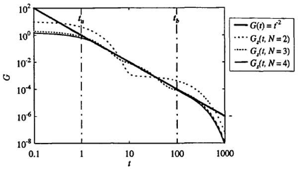
Comparison of multiexponential fits to a power-law function. Log–log plot showing fits to G = t−2 using two, three, and four exponentials with ta = 1, tb = 100, and C = 10.93, 2.16, and 1.56, respectively.
Now, let us consider as the basis function a model composed of two identical mixing chambers in series,
| (8) |
which is qualitatively a better choice for a washout function because it is a unimodal function and has a value of g = 0 at t = 0. By choosing N = 10, β = 3, ta = 1, and tb = 1000, and substituting into Eqs. (5), (6), and (7), we get the function plotted in Fig. 2. The finite sum approximation follows the power-law behavior over a range of about 3 decades in time (defined by the ratio tb/ta). Comparison of Figs. 1 and 2 demonstrates that different basis functions will give the same power-law behavior when they are summed and scaled according to Eq. (6).
FIGURE 2.
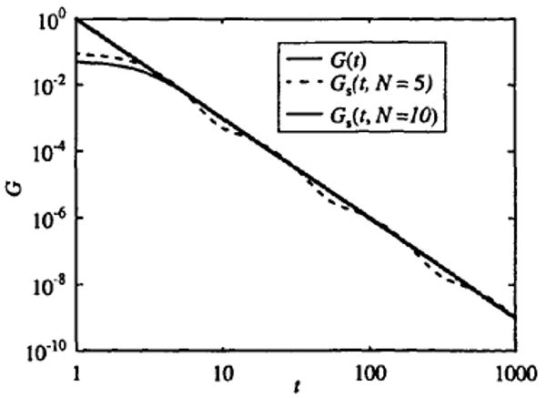
Power-law fit using unimodal basis function. Log–log plot showing a fit to G = t−3 using g(kit) = kite−kit with N = 10, ta = 1, and tb = 1000, and C = 0.1278.
Parallel Compartments can give Power-Law Behavior
The sum expressed by Eq. (6) can be related to a parallel combination of N models, each defining a probability density function of transit times. Here, each model consists of two well-stirred tanks in series. The impulse response from each system of serial stirred tanks is , where ki is proportional to the flow in the ith pathway. If we assume that the washout from the entire system hs(t) has a power-law tail, then by Eqs. (6) and (8):
| (9) |
We also know that the contribution to the concentration in the outflow from each pathway is proportional to the flow in that pathway times the probability of occurrence. Since the flow is proportional to ki, hs(t) is proportional to , where P(ki) is the relative weighting for each pathway, or its probability of occurrence in the system, and is equivalent to the probability density function of regional flows in an organ.8 Clearly P(ki) is proportional to . So the curve in Fig. 2 can be thought of as the impulse response from a system of N parallel compartments, each weighted by P(ki).
We can now think of the N parallel pathways as a discrete distribution of pathways with variable flow and constant volume. In order to relate this discrete distribution to a continuous probability density function, p(ki), note that P(ki) = Δk · p(ki), and from Eq. (7):
| (10) |
Therefore, p(ki) is proportional to . So by setting β = 3, picking ki from a uniform random distribution, and summing the flow-weighted washout for each ki, we should get the same power-law behavior shown in Fig. 2. Figure 3 shows the results of picking 1000 values of ki from a uniform distribution between 0 and 1 and summing the flow-weighted washout function according to
FIGURE 3.
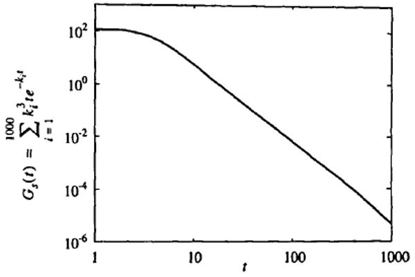
Washout due to uniformly distributed random flows. Log–log plot showing , where the ki are chosen from a uniform random distribution between 0 and 1.
| (11) |
The curve plotted in Fig. 3 has a power-law tail that clearly follows t−3. Therefore the experimentally observed behavior of water washout curves is completely explicable by the heterogeneity of the flow in the system. If we model the system by a number of parallel pathways, then we must consider a uniform distribution of flow through those pathways to get the tail of the washout curve to exhibit t−3 behavior. A different flow distribution will produce a different washout curve. In fact, this is a startlingly simple result. Uniform randomly distributed flows in parallel pipes give the power-law washout behavior shown for water washout from rabbit hearts in Ref. 1.
Power-Law Tail of Washout can be Related to Flow Heterogeneity
Consider the probability density function of flows through a parallel-flow system, p1(f), and the probability density function of pathways with a given transit time through the same system, P2(t). This p2(t) is not the same as h(t), the probability density function of transit times. The h(t) weights each element of p2(t) in proportion to the flow through the pathway. The probability of a certain flow occurring over the interval f1 to f1 + df is given by
| (12) |
for small but finite df. The probability of a transit time occurring in the interval t1 to t1 + dt is given by
| (13) |
If we assume that all pathways have the same volume V and that P1 and P2 correspond to the same interval, dt can be calculated by
| (14) |
| (15) |
| (16) |
Because they correspond to the same interval, we can set P1 and P2 equal:
| (17) |
Taking the limit as df → 0 and rearranging Eq. (17),
| (18) |
Substituting for f1 = V/t1 gives
| (19) |
Dropping the subscript on t1 and writing the washout from the system as the flow-weighted distribution of pathway transit times gives
| (20) |
or
| (21) |
where A is some constant. The washout will follow t−3 only when t3 is changing much faster than p1(V/t). Again we see that uniform flow distributions lead to approximately t−3 washout behavior!
In the above derivation, one could allow V to vary randomly. If the random variation in V were uncorrelated with flow, then the derivation would remain largely unchanged and Eq. (21) would still hold. [Imagine a discrete distribution of V values. Then the output from each set of pathways with the same volume would result in Eq. (21). These curves will sum together to give the same power law.] If f and V are correlated (which they may be), then the derivation will become more complicated, and the sensitivity of Eq. (21) to this correlation would depend upon how it is formulated.
Washout from more general flow distributions will approach t−3 behavior for limiting cases. For example, if p1 is a Gaussian distribution,
| (22) |
where tmf is the time corresponding to the mean flow and σf is the standard deviation of flows.
The washout will diminish as t−3 for all times such that
| (23) |
If σf > f̄, then the washout will follow t−3 for t > tmf, where f̄, is the mean flow. If σf is not that large, then the washout will follow t−3 when t≫tmf as the exponent of Eq. (22) approaches a constant value.
Recommendations
Evidence for the power-law form of the washout from vascular networks that we propose has come from our laboratory1,2 and others reviewed by Norwich9. Since little attention is typically paid to the long-time behavior of washout processes, more experimental measurements will be needed to test the generality of logarithmic kinetic processes of this type.
Transport and exchange models of heterogeneous flow systems usually incorporate a finite number of parallel, axially distributed or compartmental units with a fixed distribution (e.g., Gaussian) of flows through the units.8 To produce the appropriate power-law tail on washout curves, the parallel units should be equally spaced in the log transit time (or, equivalently, low flow) domain, as described by the example in the Appendix.
Many models have been developed for describing tracer exchanges between blood and tissue. Single capillary–tissue exchange unit models, even complex ones accounting for solute binding and transformation such as the oxygen models of Li et al.,7 give rise to a tail which is monoexponential. More complex multicomponent models for oxygen transport, including diffusional exchanges between arteriolar and venular volumes through intratissue diffusional exchanges, do give rise to multiexponential tails,10,12 but even these resolve into a monexponential form at very long times. Thus it is clear that all of these types of models must be extended into a network or multicapillary form if they are to provide good fits to high resolution data at late times where washout follows power-law behavior.
Appendix: Example of Power-Law Washout with Stirred Tanks in Parallel
Given a set of basis functions representing a set of stirred tanks in parallel,
| (A1) |
then we need to define the conditions under which this sums to approximately a power-law relationship h(t) ∼t−β.
The area under each kie−kit is unity. For all ai = 1.0, then the area under the summation in Eq. (A1) is determined by the ratio ε = ki+1/kj, where 0<ε<l, the length of the series and the value for β. The value of β determines the ratio γ = ai+1/ai:
For γ<1 the area under C(t) is 1 + γ+ γ2 + γ3 + ⋯ + γN, which is (1 − γN)/(l − γ). For β = 1 and for any ε, then Eq. (A1) gives a fit to t−1 to arbitrary accuracy. For higher accuracy more terms are required, so one may use ε closer to 1 and larger N, picking the highest rate constant k1 to cover the beginning of the range desired. The normalized version of Eq. (A1), when β = 1 and therefore where a1 = 1, is
| (A2) |
When β is greater than 1, so that γ is necessarily less than 1,
| (A3) |
When 0<β<1, then γ>1, and since γ · ε<1 the series converges. For β = 0, h(t) = a1t0, and the series does not converge. This stirred tank representation does not work for negative β.
References
- 1.Bassingthwaighte JB, Beard DA. Fractal 15O-water washout from the heart. Circ Res. 1995;77:1212–1221. doi: 10.1161/01.res.77.6.1212. [DOI] [PMC free article] [PubMed] [Google Scholar]
- 2.Bassingthwaighte JB, Beard DA, Li Z, Yipintsoi T. Is the fractal nature of intraorgan spatial flow distributions based on vascular network growth or local metabolic needs? In: Little C, Mironov V, Sage H, editors. Vascular Morphogenesis: In Vivo, In Vitro and In Sapiente. Boston, MA: Birkhauser; 1997. pp. 1–16. [Google Scholar]
- 3.Bassingthwaighte JB, King RB, Roger SA. Fractal nature of regional myocardial blood flow heterogeneity. Circ Res. 1989;65:578–590. doi: 10.1161/01.res.65.3.578. [DOI] [PMC free article] [PubMed] [Google Scholar]
- 4.Bassingthwaighte JB, Liebovitch LS, West BJ. Fractal Physiology. London: Oxford University Press; 1994. [Google Scholar]
- 5.Glenny R, Robertson HT, Yamashiro S, Bassingthwaighte JB. Applications of fractal analysis to physiology. J Appl Physiol. 1991;70:2351–2367. doi: 10.1152/jappl.1991.70.6.2351. [DOI] [PMC free article] [PubMed] [Google Scholar]
- 6.Hamilton WF, Moore JW, Kinsman JM, Spurling RG. Studies on the circulation. IV. Further analysis of the injection method, and of changes in hemodynamics under physiological and pathological conditions. Am J Physiol. 1932;99:534–551. [Google Scholar]
- 7.Li Z, Yipintsoi T, Bassingthwaighte JB. Nonlinear model for capillary-tissue oxygen transport and metabolism. Ann Biomed Eng. 1997;25:604–619. doi: 10.1007/bf02684839. [DOI] [PMC free article] [PubMed] [Google Scholar]
- 8.Li Z, Yipintsoi T, Caldwell JH, Zuurbier CJ, Krohn KA, Link JM, Bassingthwaighte JB. In vivo measurement of regional myocardial oxygen utilization with inhaled 15O-oxygen and positron emission tomography. Ann Biomed Eng. 1996;24(Suppl. 1):S32. [Google Scholar]
- 9.Norwich KH. Noncompartmental models of whole-body clearance of tracers: A review. Ann Biomed Eng. 1997;25:421–439. doi: 10.1007/BF02684184. [DOI] [PubMed] [Google Scholar]
- 10.Sharan M, Popel AS, Hudak ML, Koehler RC, Traystman RJ, Jones J. An analysis of hypoxia in sheep brain using a mathematical model. Ann Biomed Eng. 1988;26:48–59. doi: 10.1114/1.50. [DOI] [PubMed] [Google Scholar]
- 11.Sparacino G, Bonadonna R, Steinberg H, Baron A, Cobelli C. Estimation of organ transport function from recirculating indicator dilution curves. Ann Biomed Eng. 1998;26:128–137. doi: 10.1114/1.84. [DOI] [PubMed] [Google Scholar]
- 12.Ye GF, Jaron D, Buerk DG, Chou MC, Shi W. O2-Hb reaction kinetics and the Fahraeus effect during stagnant, hypoxic, and anemic supply deficit. Ann Biomed Eng. 1998;26:60–75. doi: 10.1114/1.81. [DOI] [PubMed] [Google Scholar]