Simultaneous Class Discovery and Classification of Microarray Data Using Spectral Analysis

Abstract

Classification methods are commonly divided into two categories: unsupervised and supervised. Unsupervised methods have the ability to discover new classes by grouping data into clusters or tree structures without using the class labels, but they carry the risk of producing noninterpretable results. On the other hand, supervised methods always find decision rules that discriminate samples with different class labels. However, the class label information plays such an important role that it confines supervised methods by defining the possible classes. Consequently, supervised methods do not have the ability to discover new classes. To overcome the limitations of unsupervised and supervised methods, we propose a new method, which utilizes the class labels to a less important role so as to perform class discovery and classification simultaneously. The proposed method is called SPACC (SPectral Analysis for Class discovery and Classification). In SPACC, the training samples are nodes of an undirected weighted network. Using spectral analysis, SPACC iteratively partitions the network into a top-down binary tree. Each partitioning step is unsupervised, and the class labels are only used to define the stopping criterion. When the partitioning ends, the training samples have been divided into several subsets, each corresponding to one class label. Because multiple subsets can correspond to the same class label, SPACC may identify biologically meaningful subclasses, and minimize the impact of outliers and mislabeled data. We demonstrate the effectiveness of SPACC for class discovery and classification on microarray data of lymphomas and leukemias. SPACC software is available at http://icbp.stanford.edu/software/SPACC/.

1. Introduction

Classification methods are commonly used for mining microarray gene expression data (Lockhart and Winzeler, 2000; Young, 2000) to gain biological insights on the class structure underlying the experimental samples and predict the relationship of new samples to the existing samples. Typical applications of classification analysis include inferring the molecular stratification of disease (Dalgin et al., 2007) or the likelihood of response to a treatment (Lin et al., 2006). Classification methods are commonly divided into two categories: unsupervised versus supervised. In unsupervised methods, such as hierarchical clustering (Eisen et al., 1998), local maximum clustering (Wu et al., 2004), self-organizing map (Kohonen, 2000) and K-means (Tavazoie et al., 1999), samples are grouped into clusters or tree structures based on the expression data. If information about the samples, typically referred to as the class labels, is provided to describe a phenotypic property, it is only used for interpreting the clustering results. Because the class label information is not involved in the clustering process, unsupervised methods have the ability to discover new classes, but they carry the risk of producing non-interpretable results. On the other hand, supervised methods—such as nearest neighbors (Duda et al., 2000), neural networks (O'Neill and Song, 2003), and support vector machine (Furey et al., 2000)—use training samples to define a rule that separates samples with different class labels. Supervised methods do not have the risk of producing non-interpretable results. However, in supervised methods, the class label information plays such an important role that it confines the supervised methods by defining the possible classes. Consequently, supervised methods do not have the ability to discover new classes. Moreover, outliers and mislabeled samples in the training data may have undesirable effect on the classification. To overcome the limitations of unsupervised and supervised methods, we propose a new classification method, which assumes the class label information is available, but uses it to a less important role so as to perform class discovery and classification simultaneously.

The proposed method is called SPACC (SPectral Analysis for Class discovery and Classification). In SPACC, the training samples are considered as inter-connected nodes that form an undirected weighted network, where an edge exists between each pairs of nodes (or samples). The weights of the connections are defined by similarity measures of the microarray expression data, independent of the class labels. Using spectral graph analysis (Pandana and Liu, 2005), the network is iteratively partitioned into two subnetworks in an unsupervised manner, forming a top-down tree-like representation of the data. The class labels are only used to examine the two subnetworks after each partitioning. If most of the nodes (or samples) in one subnetwork share the same class label, this subnetwork becomes a leaf of the tree; otherwise, the subnetwork is subject to further partitioning. Hence, the class label information supervises the partitioning process only by defining the criterion to stop partitioning the network along one branch of the tree. Once the terminals of all the branches are identified, SPACC has produced a top-down binary tree, where each terminal or leaf of the tree represents a subset of the training samples, assigned to one particular class. Several subsets may correspond to the same class, which is an indication that new classes beyond the known class labels may exist. Data outliers will be automatically partitioned into singletons. Therefore, SPACC has the potential to improve the quality of the training data, in terms of discovering new classes and identifying outliers. Classification of the testing samples can be performed using a variation of the nearest neighbor method. For each testing sample, SPACC computes its distance to those subsets, and make classification decision based on its nearest neighbor subset.

The remainder of this article is organized as follows. In Methods, SPACC is described in greater detail. In Results, the application of SPACC is illustrated on real microarray data. Discussion summarizes the advantages and limitations of SPACC, in the context of other classification methods, and is followed by Conclusion.

2. Methods

In this section, the proposed method SPACC for class discovery and classification is further described. We start with a brief summary of how spectral analysis can be applied to partition a network into two subnetworks. Then, we describe how to use the partitioning method to construct a top-down binary tree of the data, how the class labels of the training data are used to supervise the process, and how classification decisions are made.

2.1. Spectral analysis for graph partitioning

A graph (network) can be represented by G(N, A), where N is the set of nodes, and A is the adjacency matrix that describes the edges,

(1)

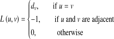
where two nodes are adjacent if there is an edge between them. For each node, the degree is defined as the number of edges that connect to it. Another way to represent a network is the Laplacian matrix, which is defined as L = D − A. D is a diagonal matrix whose diagonal elements are the degrees of the nodes. The Laplacian matrix can be written as follows:

(2)

where d_v is the degree of node v. Note that the Laplacian matrix is symmetric, and the column sums are 0.

Several properties in the spectral domain of the Laplacian matrix L are related to the connectivity of the network. All eigenvalues are non-negative. At least one eigenvalue equals zero, and the zero-valued eigenvalue may have more than one multiplicity. If it has multiplicity n, the network is disconnected and contains n disjoint components. If the network is connected, the second smallest eigenvalue is called the Fiedler value, and its associated eigenvector is called the Fiedler vector. To partition the network into two subnetworks by removing the least number of edges, an approximation of the optimal solution can be derived from the Fiedler vector (Chung, 1997), whereby its the positive entries and negative entries, respectively, correspond to the nodes of the two resulting subnetworks after the partitioning.

The above arguments can be extended to an undirected weighted network, represented by a Laplacian matrix, where each connection is represented by the negative of its weight instead of −1, and the diagonal elements are chosen such that the column sums are 0. Therefore, for an undirected weighted network, the Laplacian matrix becomes

(3)

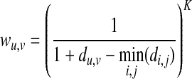
We model the experimental samples as an undirected weighted network, where each node represents a single microarray sample. An edge exists between all possible pairs of nodes (or samples), and the weight of each edge is determined by the similarity between the gene expressions of the two connected nodes,

(4)

where d_u,v is the Euclidian distance between the expression data of nodes u and v. K is a tuning parameter, similar to that in the power adjacency function (Zhang and Horvath, 2005). Higher similarity implies higher weight, while lower similarity implies lower weight. All weights are normalized into the numerical range of (0, 1).

Using the weights in equation (4), we construct the Laplacian matrix in (3) and compute its Fiedler value and Fiedler vector. The network is partitioned into two subnetworks based on the signs of the elements in the Fiedler vector. The nodes that correspond to the positive entries belong to one subnetwork; the nodes that correspond to the negative entries belong to the other subnetwork; all edges between the two subnetworks are removed. Generally, the Fiedler vector will not contain zero entries. Zero entries only occur in the Fiedler vector in special cases, such as when the network is symmetric with respect to a certain node. In such special cases, we can randomly assign the nodes with zero entries to either of the two subnetworks after the partitioning. Therefore, using the Fiedler vector, we partition the network into two subnetworks, or equivalently we divide the microarray samples into two non-overlapping subsets of samples. The partitioning is based on the distance measures of the gene expression data in an unsupervised fashion. The class label information is not incorporated at this stage.

2.2. Simultaneous class discovery and classification

In the previous subsection, we described an unsupervised method to partition a network into two subnetworks, or equivalently divide a set of microarray samples into two non-overlapping subsets. Given a set of training samples, we can iteratively apply this partitioning method to divide the training samples into a top-down full binary tree until each leaf corresponds to one training sample. However, a full binary tree would not be helpful for classification, because it does not provide a systematic decision rule (Natsoulis et al., 2005). A proper stopping criterion is needed to divide the training samples to a level that is suitable for classification.

We define the stopping criterion based on the class labels of the training samples. After each partitioning, we examine the class labels of the two resulting subsets. If the purity of a subset exceeds specified threshold, that is most samples in the subset share the same class label, we specify this subset as a leaf of the tree and stop partitioning. If a subset does not meet the stopping criterion, it is subject to further partitioning. The process iterates and results in a top-down binary tree, where each leaf corresponds to a subset of the training samples and the majority of samples in the subset share the same class label. In the resulting subsets, there may exist several subsets that correspond to the same class. This suggests new classes may exist beyond the known class labels. Data outliers will be automatically partitioned into singletons, and thus are easily identified. Resulting subsets may contain some samples that have different class labels from that of the majority. These samples may be outliers or mislabeled samples.

Since the class label information supervises the training process only by defining the stopping criterion, the class label information plays a much less important role when compared to other supervised methods. The rationale for our approach is: let the data manifest itself. If what the data shows after partitioning agrees with what we already know from the class labels, then we stop the partitioning. Otherwise, the data is revealing new information that is beyond what is captured by the known class labels, enabling us to potentially discover new classes.

For the purpose of classifying the testing samples, we choose to use a variation of the nearest neighbor algorithm. We represent each subset of the training samples by the mean expression of its members. The distance between one testing sample and one subset can be represented by the distance between the testing sample's expression data and the mean expression of the subset. For each testing sample, we make classification decision based on the subset that is nearest to the testing sample. As a comparison, in the simple nearest neighbor algorithm, the classification decision is based on the individual training sample which is nearest to the testing sample. In the proposed method, the classification decision is based on the nearest subset of training samples.

Since our method applies spectral analysis for partitioning and can perform both class discovery and classification, we call it SPACC for “SPectral Analysis for Class discovery and Classification.” SPACC is implemented in Matlab and is available at http://icbp.stanford.edu/software/SPACC/.

2.3. Related methods in the literature

Supervised methods based on classification trees (CART) (Breiman et al., 1984) also produce top-down binary trees for classification. The important distinction between these approaches and SPACC is how the class label information is used. In CART, the class labels are part of the objective function in finding the best feature and threshold for each split. CART aims to find the tree structure that best fits the known class labels. On the other hand, each partitioning step in SPACC is unsupervised, and the class labels are only used to check whether there is need to perform further partitioning. Therefore, the class labels do not affect the splits in SPACC, allowing the data to better manifest its own structure. Another difference is that, each split in CART is based on only one feature, while in SPACC each partitioning is based on all features.

Hierarchical clustering (Eisen et al., 1998) is an unsupervised method that constructs trees to explore gene expression data. Hierarchical clustering and SPACC differ in the use of class labels. Hierarchical clustering does not use class labels and SPACC does. Another difference is how the trees are constructed. Hierarchical clustering in Eisen et al. (1998) is agglomerative, building trees from bottom up. If one wish to prune a hierarchical clustering tree, additional statistical criteria are needed. On the contrary, SPACC build trees divisively, from top down. Using class label information, the divisive process is stopped at a level that is suitable for the purpose of classification.

3. Results

3.1. SPACC analysis on B-cell lymphoma data

We apply SPACC to a published gene expression dataset on diffuse large B-cell lymphoma (Alizadeh et al., 2000) to highlight the class discovery ability of SPACC. The dataset contains the expression of 4026 genes in 81 samples, which consist of 9 follicular lymphoma (FL) samples, 11 chronic lymphocytic leukaemia (CLL) samples, 42 diffuse large B-cell lymphoma (DLBCL) samples, 3 Tonsil samples, and 16 Blood B/T samples. The histologies are the class labels. In the following Examples 1–5, we consider different combinations of this data by varying the class label information. We will demonstrate that when the training samples contain subclasses which are not represented in the class label information, SPACC is able to identify the presence of subclasses.

Example 1

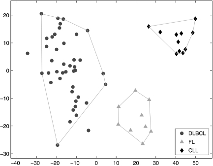
We first construct a training set, which contains the three B-cell malignancies: the FL, CLL, and DLBCL samples. All 4026 genes are considered. This training set, together with the correct class labels, are input to SPACC. The result is shown in Figure 1. The horizontal and vertical axes are the coefficients of the first two principal components of the training data. Each node represents one training sample and its shape indicates the input class label: circles represent the 42 DLBCL samples, triangles represent the 9 FL samples, and diamonds represent the 11 CLL samples. Using SPACC, we partition the training samples into three subsets and two outliers, which are shown by the polygons. The three resulting subsets are consistent with the input class labels.

Fig. 1.

SPACC applied to B-cell lymphoma gene expression data, example 1 in Results. The horizontal and vertical axes are the coefficients of the first two principal components. The shape of the nodes represents the input class labels. SPACC divides the samples into three subsets, which are indicated by the polygons. The resulting subsets are consistent with the input class labels.

Example 2

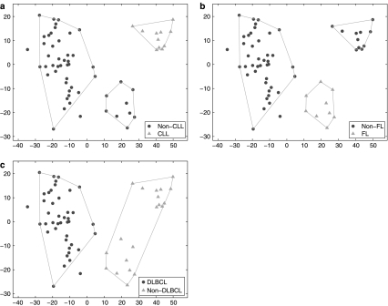
We consider the same training data as in Example 1, but vary the class label information to represent only two of the three classes as known. In Figure 2a, the class labels are chosen to represent only two classes. Circles are non-CLL samples (both DLBCL and FL) and triangles represent CLL samples. The SPACC result is shown by the polygons. Although there are only two classes in the input class labels, without knowing the subclasses in the non-CLL class, SPACC correctly divides the training samples into three subsets, one corresponding to the CLL class and the other two corresponding to the non-CLL class. In this example, other supervised classification methods will only learn the difference between CLL and non-CLL, and assign a testing sample to either of the two. However, SPACC is able to discover the subclasses beyond the known class labels, and classify testing samples into three categories, CLL, non-CLL-1 and non-CLL-2. The two non-CLL classes correctly capture the difference between DLBCL and FL in the non-CLL class.

Fig. 2.

SPACC applied to B-cell lymphoma data, examples 2–4. (a) The shapes of the nodes indicate that input class labels only distinguish CLL from non-CLL. SPACC divides the samples into three subsets, which are shown by the polygons. Without prior knowledge of the subclasses in the non-CLL class, SPACC is able to divide the non-CLL samples into two subsets, which correctly captures the difference between FL and DLBCL in the non-CLL class. (b) When the input class labels contain only two classes (FL and non-FL), SPACC correctly divides the non-FL class into two subsets, corresponding to CLL and DLBCL respectively. (c) When the input class labels represent DLBCL and non-DLBCL, SPACC does not identify the substructures within the non-DLBCL class, suggesting a high degree of similarity between FL and CLL compared to DLBCL.

Example 3

We consider the same training data as in Example 1, but vary the class labels for DLBCL and CLL. In Figure 2b, the input class label contains two classes FL and non-FL, where non-FL contains both DLBCL and CLL samples. Without knowing the subclasses in the non-FL class, SPACC divides the training samples into three subsets, where the two subtypes in the non-FL class are successfully identified.

Example 4

We consider the same training data as in Example 1, but vary the class labels for FL and CLL. In Figure 2c, the input classes are DLBCL and non-DLBCL (FL and CLL). SPACC does not identify the FL and CLL subtypes in the non-DLBCL class. The results suggest that FL and CLL are more similar to each other than either is to DLBCL. This finding was confirmed in Alizadeh et al. (2000), which showed that both FL and CLL are relative indolent malignancies with low proliferation rates, while DLBCL is more aggressive with rapid proliferation.

Example 5

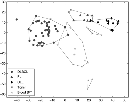
We apply SPACC to all 81 samples in Alizadeh et al. (2000), with the correct class labels. As shown in Figure 3, samples are marked using five different shapes, indicating that samples are categorized into five classes by the input class labels. The horizontal and vertical axes again are the coefficients of the first two principal components of the training data. Since we are considering more training samples, the principal components are different from those in Examples 1–4, and Figure 3 appears different from Figures 1 and 2. Figure 3 shows that SPACC divides the training data into six subsets. The FL, CLL and DLBCL classes are correctly separated. One of the three Tonsil samples is grouped with the DLBCL samples and the other two are grouped with the FL samples. Moreover, the Blood B/T samples (stars) are divided into three subsets. Interestingly, in Alizadeh et al. (2000), it is noticed that the three stars in the subset at the bottom correspond to blood T-cells; the three stars in the upper right subset are resting blood B-cells; and the rest are activated blood B-cell samples. Therefore, separating the Blood B/T samples into the three subsets in Figure 3 is biologically meaningful.

Fig. 3.

SPACC applied to the B-cell lymphoma data, example 5 in Results. The shapes of the nodes indicate that the samples are categorized into five classes by the input class labels. The polygons show the subsets obtained by SPACC. The FL, CLL and DLBCL classes are correctly separated. The three Tonsil samples are grouped with either DLBCL or FL. Interestingly, the Blood B/T samples (stars) are divided into three subsets, which correspond to blood T-cells, activated blood B-cells, and resting blood B-cells, respectively. Therefore, SPACC successfully identifies subclasses in the Blood B/T class.

Note that in Figure 3, some subsets appear to overlap, because we use the first two principal components to display the data. If we examine other principal components, we will notice that the different subsets do not overlap.

3.2. SPACC analysis on ALL-AML data

To demonstrate SPACC's ability to perform class discovery and classification, we apply SPACC to the ALL-AML dataset (Golub et al., 1999). This dataset contains two classes of samples, acute lymphoblastic leukemia (ALL), and acute myeloid leukemia (AML). We choose this dataset because it contains a training set (27 ALL, 11 AML) and an independent testing set (21 ALL, 14 AML). In the SPACC analysis, we consider the top 1000 genes that are most differently expressed in the two classes in the training samples.

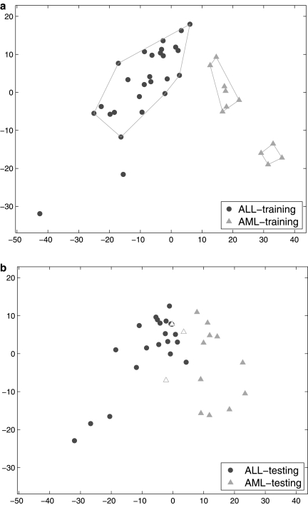
We input the 38 training samples and the corresponding class labels (ALL vs. AML) into SPACC. The training samples are shown in Figure 4a, where the horizontal and vertical axes are the coefficients of the first two principal components of the training samples. Circles represent the ALL samples, and triangles represent the AML samples. As demonstrated by the resulting polygons, SPACC divides the training samples into three subsets and two outliers. Interestingly, the AML training samples are divided into two subsets. According to the clinical information provided in Golub et al. (1999), we are unable to tell the difference between the two subsets of the AML training samples. However, by visually inspecting the testing samples in Figure 4b, we can observe similar structure in the testing set, which supports the possibility that the two subsets of AML training samples are biologically different. Note that, in order to make Figure 4a and Figure 4b comparable, we project the testing samples to the subspace spanned by the first two principal components of the training samples.

Fig. 4.

(a) Training samples of the ALL-AML data. The polygons indicate the subsets obtained by SPACC, where the AML samples are divided into two subclasses. (b) Testing samples. SPACC achieves 91.4% classification accuracy, which is higher than the nearest neighbor method. The incorrectly classified testing samples are highlighted. SPACC offers more information than other supervised classifiers. Other supervised methods only classify a testing sample to either the ALL class or the AML class. On the other hand, SPACC is able to classify testing samples into three categories (ALL, AML-1, and AML-2), which may correspond to biologically meaningful subtypes.

For the purpose of classifying each testing sample, we compute the distance between the testing sample and the mean expression of each of the three subsets. The classification decision is made based on the class label of the nearest subset. Therefore, the proposed method is a nearest-subset-center method. The classification accuracy of SPACC is 91.4%. In Figure 4b, the incorrectly classified testing samples are highlighted. As a comparison, we apply the simple nearest neighbor algorithm, and obtain 82.9% accuracy. One may argue that, the improved performance of SPACC over the near neighbor algorithm is due to the fact that SPACC is based on the nearest subset of training samples, while the nearest neighbor algorithm is based on the nearest individual training sample. To address this point, we examine a nearest-class-center method, where we compute the distance between a testing sample and the mean expression of each class in the training set define by the training labels, and make classification decision based on the nearest class. The nearest-class-center method gives an accuracy of 88.6%, which is still lower than SPACC. This result also supports our previous argument that, dividing the AML training samples into two subsets is likely to be biologically relevant.

We are not claiming that SPACC will outperform all other classifiers in terms of classification accuracy. But we are claiming that its class discovery feature enables SPACC to provide more information than other supervised classification methods. In this example, other supervised methods only classify a testing sample to either the ALL class or the AML class. However, SPACC is able to classify testing samples into three categories (ALL, AML-1, and AML-2), where the two AML subclasses may correspond to biologically meaningful subtypes.

4. Discussions

We introduced a novel classification method, SPACC, and demonstrated its class discovery ability and classification performance on gene expression microarray data for B-cell lymphoma and ALL-AML. While other methods may outperform SPACC for either class discovery or classification, we are not aware of another method like SPACC that can simultaneously perform class discovery and classification. This ability allows SPACC to provide more information than other classification methods.

Feature selection is an important issue in SPACC, as it is in other classification approaches. In SPACC, we convert the gene expression data to a similarity matrix, which is further converted to the weights in the Laplacian matrix. Since the number of genes under consideration does not affect the size of the Laplacian matrix, in theory we are able to handle a large number of genes. However, in practice, we have to be careful about feature selection. Because SPACC partitions samples into subsets based on the distances among the expression data, when there are too many irrelevant gene features, the distances among samples will be more noisy and SPACC will lose its ability to separate different classes. Therefore, even though we do not need to limit the number of genes that can be analyzed by SPACC, we need to ensure that the majority of selected features are relevant to the classification problem.

We described SPACC as a supervised approach. However, if we remove the stopping criterion, SPACC becomes an approach of unsupervised hierarchical clustering. Different from the agglomerative hierarchical clustering method in Eisen et al. (1998), SPACC is divisive and produces a top-down binary tree. If we define a data-driven stopping criterion, we will be able to build an unsupervised clustering method that does not need to require prior knowledge of the number of clusters. We pursued this idea by using stopping criteria derived by thresholding the Fiedler value at each partitioning, or via the statistics that evaluate between- and within-subset variances. However, we found that these stopping criteria were not universally applicable to a variety of datasets. Related discussions can be found in CLICK developed in Sharan et al. (2003).

5. Conclusion

We propose a novel classification method SPACC for simultaneous class discovery and classification of microarray data. Compared to other supervised methods, SPACC utilizes the class label information to a lesser extent, so as to perform class discovery and classification simultaneously. In addition to identifying new classes that may provide new biological insights, SPACC can be useful in identifying outliers and mislabeled training samples. To the best of our knowledge, SPACC is the first approach that can simultaneously perform class discovery and classification. Using two publicly available gene expression microarray datasets, we demonstrate SPACC's ability for class discovery and classification.

Acknowledgments

This work was supported by the NCI Integrative Cancer Biology Program (ICBP) (grant U56 CA112973).

Disclosure Statement

No competing financial interests exist.

References

- Alizadeh A.A. Eisen M.B. Davis E.E., et al. Distinct types of diffuse large b-cell lymphoma identified by gene expression profiling. Nature. 2000;403:503–511. doi: 10.1038/35000501. [DOI] [PubMed] [Google Scholar]
- Breiman L. Friedman J. Stone C., et al. Classification and Regression Trees. Chapman & Hall/CRC; Boca Raton, F: 1984. [Google Scholar]
- Chung F.R.K. Spectral Graph Theory (CBMS Regional Conference Series in Mathematics, No. 92; American Mathematical Society; New York. 1997. [Google Scholar]
- Dalgin G. Alexe G. Scanfeld D., et al. Portraits of breast cancer progression. BMC Bioinform. 2007;8:291. doi: 10.1186/1471-2105-8-291. [DOI] [PMC free article] [PubMed] [Google Scholar]
- Duda R.O. Hart P.E. Stork D.G. Pattern Classification. 2nd. Wiley-Interscience; New York: 2000. [Google Scholar]
- Eisen M.B. Spellman P.T. Brown P.O., et al. Cluster analysis and display of genome-wide expression patterns. Proc. Natl. Acad. Sci. USA. 1998;95:14863–14868. doi: 10.1073/pnas.95.25.14863. [DOI] [PMC free article] [PubMed] [Google Scholar]
- Furey T.S. Christianini N. Duffy N., et al. Support vector machine classification and validation of cancer tissue samples using microarray expression data. Bioinformatics. 2000;16:906–914. doi: 10.1093/bioinformatics/16.10.906. [DOI] [PubMed] [Google Scholar]
- Golub T.R. Slonim D.K. Tamayo P., et al. Molecular classification of cancer: class discovery and class prediction by gene expression monitoring. Science. 1999;286:531–537. doi: 10.1126/science.286.5439.531. [DOI] [PubMed] [Google Scholar]
- Kohonen T. Self-Organizing Maps. Springer; New York: 2000. [Google Scholar]
- Lin S. Devakumar J. Kibbe W. Improved prediction of treatment response using microarrays and existing biological knowledge. Pharmacogenomics. 2006;7:495–501. doi: 10.2217/14622416.7.3.495. [DOI] [PubMed] [Google Scholar]
- Lockhart D.J. Winzeler E.A. Genomics, gene expression and dna arrays. Nature. 2000;405:827–836. doi: 10.1038/35015701. [DOI] [PubMed] [Google Scholar]
- Natsoulis G. El Ghaoui L. Lanckriet G.R., et al. Classification of a large microarray data set: algorithm comparison and analysis of drug signatures. Genome Res. 2005;15:724–736. doi: 10.1101/gr.2807605. [DOI] [PMC free article] [PubMed] [Google Scholar]
- O'Neill M.C. Song L. Neural network analysis of lymphoma microarray data: prognosis and diagnosis near-perfect. BMC Bioinform. 2003;4:13. doi: 10.1186/1471-2105-4-13. [DOI] [PMC free article] [PubMed] [Google Scholar]
- Pandana C. Liu K.J.R. Maximum connectivity and maximum lifetime energy-aware routing for wireless sensor networks. IEEE GLOBECOM ’05. 2005;2:5–10. [Google Scholar]
- Sharan R. Maron-Katz A. Shamir R. Click and expander: a system for clustering and visualizing gene expression data. Bioinformatics. 2003;19:1787–1799. doi: 10.1093/bioinformatics/btg232. [DOI] [PubMed] [Google Scholar]
- Tavazoie S. Hughes J.D. Campbell M.J., et al. Systematic determination of genetic network architecture. Nat. Genet. 1999;22:281–285. doi: 10.1038/10343. [DOI] [PubMed] [Google Scholar]
- Wu X. Chen Y. Brooks B., et al. The local maximum clustering method and its application in microarray gene expression data analysis. EURASIP J. Appl. Signal Process. 2004;2004:53–63. [Google Scholar]
- Young R.A. Biomedical discovery with DNA arrays. Cell. 2000;102:9–15. doi: 10.1016/s0092-8674(00)00005-2. [DOI] [PubMed] [Google Scholar]
- Zhang B. Horvath S. A general framework for weighted gene co-expression network analysis. Stat. Appl. Genet. Mol. Biol. 2005;4 doi: 10.2202/1544-6115.1128. article 17. [DOI] [PubMed] [Google Scholar]