Optimization of a Microfluidic Mixing Process for Gene Expression-Based Bio-dosimetry

Abstract

In recent decades advances in radiation imaging and radiation therapy have led to a dramatic increase in the number of people exposed to radiation. Consequently, there is a clear need for personalized biodosimetry diagnostics in order to monitor the dose of radiation received and adapt it to each patient depending on their sensitivity to radiation exposure (Hall E.J. and Brenner D. J., 2008). Similarly, after a large-scale radiological event such as a dirty bomb attack, there will be a major need to assess, within a few days the radiation doses received by tens of thousands of individuals. Current high throughput devices can handle only a few hundred individuals per day. Hence there is a great need for a very fast self-contained non-invasive biodosimetric device based on a rapid blood test.

This paper presents a case study where regression methods and designed experiments are used to arrive at the optimal settings for various factors that impact the kinetics in a biodosimetric device. We use ridge regression to initially identify a set of potentially important variables in the mixing process which is one of the critical sub systems of the device. This was followed by a series of designed experiments to arrive at the optimal setting of the significant microfluidic cartridge and piezoelectric disk (PZT) (D. Sadler, F. Zenhausern, U.S. Patent 6,986,601; Lee, S. Y., Ko, B., Yang, W., 2005) related factors. This statistical approach has been utilized to study the microfluidic mixing to mix water and dye mixtures of 70 μl volume. The outcome of the statistical design, experimentation and analysis was then exploited for optimizing the design, fabrication and assembly of the microfluidic devices. As a result of the experiments that were performed, the system was fine tuned and the mixing time was reduced from 5.5 minutes to 2 minutes.

1. INTRODUCTION

Radiation exposure in the US is increasing yearly as advent of powerful tests and procedures is adding to the radiation exposure of the population. Biological tests to measure the radiation exposure would be most desirable for monitoring the dose of radiation received by oncology patients, as well as potential victims of an act of radiologic terrorism such as a dirty bomb attack. This case study describes the application of regression analysis and designed experiments to the subsystem of a new miniaturized biodosimeter system suitable for rapid screening and triage of individuals who may have been exposed to low dosage radiation (typically < 2Gy) versus non radiated individuals. Gene expression-based biosignatures (Paul S. and S.A. Amundson, 2008) were identified and an enzymatic assay was developed to provide rapid detection of biological exposure to low dose radiations. The quantitative Nuclease Protection (qNPA) chemistry (Martel, R., Botros, I., Rounseville, M., et al, 2002) was developed to be integrated into a microfluidic platform (Liu, R. H., Lenigk, R., Grodzinski, P., 2003) for enhancing its reaction kinetics by using several mixing steps for efficient nucleic acid hybridization (Liu, R. H., Yang, J., Pindera, M. Z., Athavale, M., Grodzinski, P., 2002). The development of a fully integrated microfluidic system suitable for automating all the laboratory operations necessary to perform the qNPA measurement requires great control of small volume of fluids in a series of microfluidic components. These components comprise microchannels, micro-pumps, micro-valves and micro-mixers. The introduction of assay reagents and target nucleic acids in microchannels are sensitive to near-surface effects that occur in fluids at the microscale level. Due to low Reynolds numbers, mixing fluids in microchannels is challenging. However, bubble-induced acoustic microstreaming (R. Liu, R. Lenigk, P. Grodzinski, F. Zenhausern, 2003) has been demonstrated as a promising configuration for active mixing (J. Xie, D. Attinger, 2007) but its design and operating parameters have not been fully characterized and optimized.

We illustrate a development approach using ridge regression analysis and designed experiments for characterizing and optimizing the design and fabrication of the microfluidic mixer device for enhanced kinetics and ultimately speeding up the biodosimetric measurement.

2. SYSTEM DESCRIPTION

Acoustic microstreaming (Elder, S. A., 1959; Willard, G. W., 1954; Kolb, J., Nyborg, W. L., 1956; Yang, Z., Goto, H., Matsumoto, M., Maeda, R., 2000) used to create Piezo-electric transducer (PZT) mixing is a promising option for mixing fluids in the microfluidic environment (Yu, H., Kwon, J. W., Kim, E. S., 2006). The chambers used to test water-dye mixing have been designed in accordance with the final assay volume specifications. An oscilloscope was used to generate the required frequency and frequency range with the desired sweep rate. The consistency of the water and dye mixture is maintained to meet the consistency of the final assay. Initial set of experiments were run on cartridges with 9 chambers. Each of these chambers had dimensions to contain a volume of 70 micro-liters. Some preliminary experiments had been run to arrive at the ranges for the different variables involved in the experiment. The variables for the experiments are divided into two main categories, those that are PZT related and those that are Chamber related. These variables were varied within a working range and mixing time for water and dye was noted. The regression analyses were done using Minitab and Matlab. The designed experiments were constructed and analyzed using Design Expert.

3. OVERVIEW OF ANALYSIS METHODS

Initially since the system was not well understood, the important factors in the system were unknown. A series of experiments were conducted with the intention of identifying the variables that affect the response; mixing time. When this project was begun, the results from 23 initial experiments were available. There were 184 experimental runs performed in these 23 experiments. These tests had been performed without the benefit of any designed experiment approach. Hence the presence of confounding, noise factors, and random error in the dataset is inevitable. However, these experiments did shed some light on the important variables in the process. The dataset was therefore used to perform regression analysis in order to understand the amount of variability explained by the known, controllable variables identified by these initial experiments.

Initially the data obtained contained 10 variables and as the understanding of the system was improved, some variables were removed and others were added. This led to a final list of 14 variables out of which one variable (volume of the chamber) was removed as it was redundant in the presence of diameter and depth of chamber. Three of the 13 variables identified were qualitative and were converted to indicator variables in order to be able to use these variables in the regression analysis. This resulted in 184 observations, 13 variables and one response (mixing time).

Regression analysis was performed on the data set and a subset of significant variables was identified. This analysis resulted in some of the variables being dropped from further studies as they did not appear to contribute significantly to the mixing time. This subset of variables was then used to conduct designed experiments to minimize the mixing time. Response surface methodology was employed to optimize the process and arrive at levels of the variables such that the output was not affected by the noise in the system. Ultimately a robust process was developed where the response (mixing time) is not affected by the known and unknown noise variables and is optimized for levels of the known, controllable variables.

4. REGRESSION ANALYSIS

Regression analysis is very useful in studying undesigned datasets to identify potentially important variables and to provide information that can lead to hypotheses that can be explored with designed experiments. Three of the variables are qualitative and since one of them has three levels and the other two have two levels each, these three variables are converted into four indicator variables. The multiple linear regression resulted in an R² predicted value of 32.98% and the variance inflation factors (VIFs) for four of the variables are greater than ten, viz. Rate of Sweep, Frequency Range, Piezo Offset and Static/Sweep. Since the dataset shows the presence of multicollinearity, multiple linear regression would likely result in an inadequate model for the data. Principal component regression and ridge regression (Montgomery, D. C., Peck, E. A., Vining, G. G., 2006) are the two possible regression analysis methods which are more likely to give better results without being influenced by the multicollinearity.

Principal component analysis (PCA) was done on the dataset and the components were selected based on the variation explained by the components. The scree plot and the eigenvalue analysis show that the first four components explain 78.2% of the variation. Hence these four components are selected and principal component regression analysis is done. The model built using the principal components as variables results in an R-Sq (adj) value of 22%. This indicates that perhaps higher order terms need to be included into the analysis to explain the variation in mixing time. All the pure quadratic and two-factor interaction terms are included, and then PCA regression is done. PCA shows that the first six components account for 85% of the variation. Hence only these six principal components are included in the principal component regression analysis. The R-Sq (adj) value of the regression model fit using the six principal components is 36.5%.

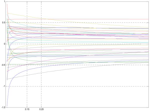
Since the amount of variability explained is very low, ridge regression was considered to understand the dataset better and better explain the variability. The ridge trace is used to identify the value of the biasing parameter at which the coefficients will stabilize. Cross validation is used, where the data (184 observations) is divided into four equal parts. One part is excluded each time and ridge regression is performed over a range of biasing parameter from zero to one in increments of 0.025. The residual average sum of squares for all folds of the data are calculated and plotted against the bias parameter terms.

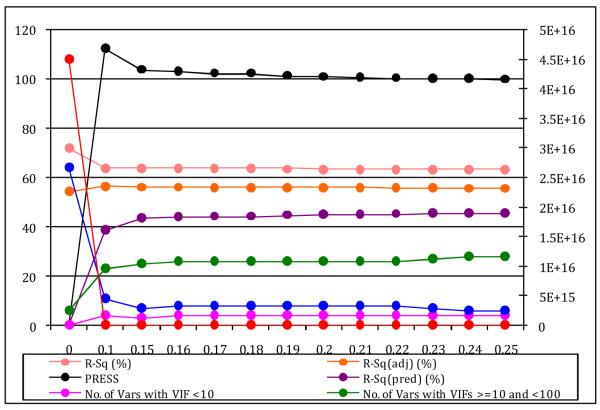
Using the ridge trace 37 variables are shortlisted for further study. These variables were chosen based on their stability in the ridge trace and because their stabilized values were not close to zero. These variables are as referred to in the regression equation that follows. The ridge trace for this reduced model is as shown in Figure 1. The values of the biasing parameter (k) ranging from 0.15 to 0.25 in increments of 0.01 are used to arrive at the final ridge regression model. The value of k which gives the best fit for the dataset is then used in the final model. Since all the critical statistics are stabilizing at 0.15 as seen in Figure 2, this is chosen as the final value of k. The results of the regression analysis are given in Table 1 and Table 2.

FIGURE 1.

Ridge trace for the reduced model (37 variables)

FIGURE 2.

Statistics for varying values of the biasing parameter

TABLE 1.

Final results of the ridge regression using k = 0.15

S = 0.602858	R Sq = 63.7%	R Sq(adj) = 56.1%
PRESS = 103.762	R Sq(pred) = 43.30%

TABLE 2.

Analysis of Variance

Source	DF	SS	MS	F	P
Regression	38	116.4931	3.0656	8.44	0.000
Residual Error	183	66.5091	0.3634
Total	221	183.0022

The regression equation is:

$$\begin{array}{cc}\hfill \widehat{y}=& -0.012-0.842x_2-0.137x_3+0.332x_6+0.288x_7-0.301{x_1}^2+1.330{x_5}^2-0.114{x_6}^2-0.252{x_7}^2\hfill \\ \hfill & -0.810{x_{12}}^2+0.369{x_1}^3+0.006{x_3}^3+0.040{x_6}^3-0.791x_2{x}_3+0.246x_2{x}_4+0.035x_2{x}_7+0.105x_2{x}_8\hfill \\ \hfill & +0.060x_2{x}_{13}+0.145x_2{x}_{14}+0.470x_3{x}_7+0.564x_3{x}_8+0.577x_3{x}_9-0.573x_3{x}_{11}+0.462x_3{x}_{14}\hfill \\ \hfill & +0.077x_3{x}_{15}+0.377x_4{x}_6-0.474x_4{x}_{12}+0.078x_5{x}_6-0.780x_5{x}_{12}-0.339x_5{x}_{14}+0455x_6{x}_{12}\hfill \\ \hfill & -0.531x_6{x}_{13}+0.638x_6{x}_{14}-0.028x_7{x}_8-0.523x_7{x}_{12}+0.481x_8{x}_{12}+0.22x_8{x}_{13}+0.0648x_8{x}_{15}\hfill \end{array}$$

The mixing time is to be minimized, and this leads to the suggested settings for the significant variables shown in Table 3. Some of these factors were finalized due to practical experimental reasons even before all the runs were completed. The regression equation suggests COC, but due to practical reasons, polycarbonate (PC) was the final choice. Even though the ridge regression results in a reasonably satisfactory model, it still explains only around 56.1% of the variability. It also contains a relatively large number of variables and high-order terms.

TABLE 3.

Variable settings

Variable	Name	Level	Experiment
x1	Cartridge Number (Experimental Variation)
x2	PZT diameter (mm)	Smaller Diameter
x3	No of times used before	Lesser No. of times used
x4	Sweep rate (sec)	Smaller rate of sweep	Expt #5
x5	Frequency range (kHz)	Smaller range	Expt #3, Expt #4, Expt #5
x6	Frequency at which the best mixing occurs (kHz)	Lower frequency
x7	Diameter of the chamber (mm)	Smaller Chamber Diameter	Expt # 1
x8	Depth of the chamber (mm)	Smaller Chamber Depth	Expt #1, Expt #3,
x9	Depth of the air pockets (mm)	Smaller Air-pocket depth	Expt #1, Expt #2
x10	Pitch of the air pocket (mm)	No significant effect	Expt #2, Expt #3, Expt #4
x11	PZT offset (mm)	Larger PZT Offset	Expt # 1
x12	Condition of PZT (single - 0/double – 1)	Double sided
x13, x14	Fixed (01) /Manual (00) /Auto Range (10)	10 – Auto range
x15	Material Used (COC – 0, PC – 1)	COC -0

5. REGRESSION ANALYSIS RESULTS

Linear regression, PCA regression and ridge regression gave varied results. Linear regression did not give good results as there is high multicollinearity between the variables. PCA regression explained only 36.5% of the variation even after including the interactions and the squared terms. Ridge regression gives the best results but it explains only 56.1% of the variation. This is inadequate to develop a robust system. It is known that the variables studied during these initial 23 experiments were not completely controlled. There was a lot of noise in the system which needs to be studied in a more controlled environment. The ridge regression equation and the values as suggested above for each of the factors was used to identify the important factors and their working ranges. These factors were used in a series of designed experiments to arrive at the optimum settings of the variables to optimize the mixing time. The designed experiments were conducted to create a robust environment which would be able to minimize the mixing time even in the presence of known or unknown uncontrollable noise.

6. OPTIMIZATION USING DESIGNED EXPERIMENTS

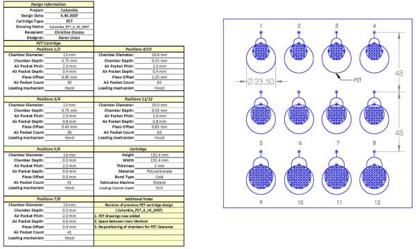
The results of the ridge regression were used to arrive at a smaller subset of factors which need to be studied. The others were held constant based on the results of the regression analysis. Designed experiments were then used to optimize the factors which have a significant effect on the mixing. The cartridge variables, viz. Chamber Diameter, Chamber Depth, Air Pocket Depth and Piezo offset, are the variables chosen initially to be studied using designed experiments. These variables are chosen based on the regression results and the process knowledge of the experimenter. Chamber depth is dependent on the chamber diameter as volume of the chamber is to be held constant and Piezo offset is dependent on the chamber depth, therefore these two factors are dropped from the experiment. A typical cartridge used to conduct the experiments is as shown in Figure 3. The dimensions of the various chambers on the cartridge are varied as per the requirements of the designed experiment. The data tables are made available as part of the appendix in an extended version of the paper¹.

FIGURE 3.

Cartridge Design

6.1. DESIGNED EXPERIMENTS - CARTRIDGE VARIABLES

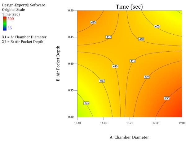
All the other controllable factors are held constant at a level that would optimize the mixing time. A D-optimal design is chosen as the design for this experiment as the design space is neither a sphere nor a cube. The model assumed to create the D-Optimal design (Experiment #1) is a full quadratic model in the two factors. A D-optimal design (Myers, R. H., Montgomery, D. C., 2002) with 2 blocks (number of cartridges used) is run with each block containing 30 (number of chambers per cartridge) experiments. The two factors in this experiment are chamber diameter and air pocket depth. Chamber diameter is varied between 12.4mm to 19mm and air pocket depth is varied from 0.3mm to 0.5 mm. Though these two factors are continuous factors, the restrictions on the chamber volume and the thickness of the material used, restricts the values that these two factors can take to three specific values (12.4, 14.7, 19.00) for chamber diameter and two values (0.3, 0.5) for air pocket depth. There were 6 possible combinations of the factor levels and 10 replicates were run at each combination in this experiment. The experiment is a blocked design as all the experiments were run on two cartridges and they were run over a period of 2 days. Once the experiments were completed, the data was analyzed and it was observed that the data are not normally distributed and a power transformation with λ = 2.18 was used. The sequential sum of squares in Table 4 indicates that a two factor interaction model is a good model for the data. The results of the ANOVA are given in Table 5. It shows that only the interaction between the two factors has a significant effect on the mixing time but the main effects are retained to maintain a hierarchical model. The final equation in terms of actual factors is

$${\widehat{\left(\text{Time}\right(\sec \left)\right)}}^{2.18}=-2057389+167715.86\ast \text{Chamber Diameter}+5970912.95\ast \text{Air Pocket Depth}-391077.63\ast \text{Chamber Diameter}\ast \text{Air Pocket Depth}$$

This equation and the contour plot in Figure 4 indicate that the Chamber diameter and air pocket depth have to decrease together to minimize the mixing time. Based on the results of the above experiment, chamber diameter was fixed at 13mm and chamber depth at 0.60mm. This was based both on the experimental results and the manufacturing feasibility of the chamber dimensions.

TABLE 4.

Sequential Model Sum of Squares

Source	Sum of Squares	df	Mean Square	F Value	p-value Prob > F
Mean vs Total	1.526E+013	1	1.526E+013
Block vs Mean	4.631E+010	1	4.631E+010
Linear vs Block	5.807E+010	2	2.903E+010	0.39	0.6808
2FI vs Linear	6.866E+011	1	6.866E+011	10.75	0.0018
Quadratic vs 2FI	1.216E+011	1	1.216E+011	1.94	0.1699
Cubic vs Quadratic	3.362E+010	1	3.362E+010	0.53	0.4695
Residual	3.358E+012	53	6.335E+010
Total	1.957E+013	60	3.261E+011

TABLE 5.

ANOVA for the 2FI model

Source	Sum of Squares	df	Mean Square	F Value	p-value Prob > F
Block	4.63E+10	1	4.63E+10
Model	7.45E+11	3	2.48E+11	3.88646	0.0137
A-Chamber Diameter	5.72E+10	1	5.72E+10	0.8951 2	0.3482
B-Air Pocket Depth	1.69E+10	1	1.69E+10	0.26440	0.6092
AB	6.87E+11	1	6.87E+11	10.7502	0.0018
Residual	3.51E+12	55	6.39E+10
Lack of Fit	2.84E+11	7	4.06E+10	0.60407	0.7495
Pure Error	3.23E+12	48	6.73E+10
Cor Total	4.3E+12	59

FIGURE 4.

Contour plot of Chamber diameter and Air pocket depth

PZTs from different manufacturers were tested to identify whether all of the PZTs behaved the same. It was observed that there was a significant difference in the operating frequency range of the PZTs. The Omega PZTs had a higher operating frequency range and the APC international PZTs have a lower operating frequency range. The results from the experiments conducted with APC International 23.5 diameter PZTs and Omega 23.5 diameter PZTs were used to design another set of experiments where air pocket depth and pitch were varied while using the dimensions for chamber depth and chamber diameter arrived at from the above experiment.

A 2¹ ×3¹ full factorial design (Montgomery, D. C., 2005) is used and a 24 run experiment is designed with 2 blocks (Experiment #2). The two blocks represent the cartridge and the time, as the 24 runs need to be run on two different cartridges over a period of time. The variation between the cartridges is a known noise factor and needs to be blocked. The air pocket depth is varied over two levels (0.4, 0.8) and the air pocket pitch is varied over three levels (1.0, 1.5, and 2.0). The sequential sum of squares analysis shows that the linear model is a good fit for the model. The results of the ANOVA in table 6 show us that air pocket pitch and its square are the significant factors. The dimensional chamber characteristics that results in optimized mixing are shown in Table 7.

TABLE 6.

ANOVA for the Air Pocket Pitch and it’s square

Source	Sum of Squares	df	Mean Square	F Value	p-value Prob > F
Block	378.47	1	378.47
Model	137.12	2	68.56	5.99	0.0091
A-Air Pocket Pitch	84.11	1	84.11	7.35	0.0134
A2	53.02	1	53.02	4.63	0.0437
Residual	228.80	20	11.44
Lack of Fit	39.19	8	4.90	0.31	0.9475
Pure Error	189.61	12	15.80
Cor Total	744.40	23

TABLE 7.

Cartridge dimensional factor levels

Chamber Diameter	13 mm
Chamber Depth	0.64 mm
Air Pocket Pitch	1.68 mm (>2 needs to be tested to see if the graph shows a downward trend outside the already tested design space)
Air Pocket Depth	0.4 – 0.8 mm

The results of the above experiments indicate that blocking is significant. This was an expected result, as variation from cartridge to cartridge is a known nuisance factor. One of the goals of the experiments is to be able to identify levels of the factors which would minimize the effect of this factor on the response.

6.2. DESIGNED EXPERIMENTS - CARTRIDGE & PZT VARIABLES

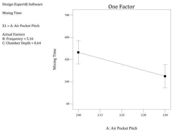
Using the outcome from the confirmation experiment analysis, another designed experiment was run to test different frequency ranges, chamber depths and increased air pocket pitches. From this experiment (Experiment #3) the best air pocket pitch was finalized as 2.5 mm as shown in the one factor plot in Figure 5. The other two factors did not have a significant effect on the response.

FIGURE 5.

One Factor plot of Air Pocket Pitch

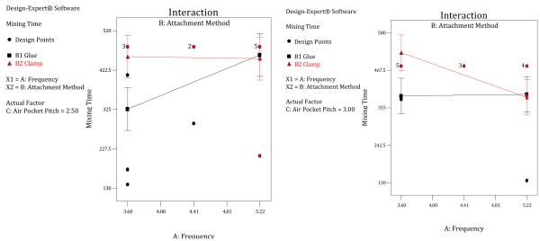
Currently all PZTs are glued onto the cartridge. There may be variables introduced from the attachment method. This is done by hand, and while placement, pressure and glue amount try to be maintained, it is difficult to maintain consistency. A new experiment was used to test an alternative method of attachment using a clamp. A 2² ×3¹ factorial experiment was used to test 2 levels of the attachment method; frequency range from 3.6 KHz to 5.22 KHz and an air pocket pitch ranging from 2.5mm to 3.0 mm (Experiment #4). 30 runs were run in 2 blocks for the 2 cartridges used. The ANOVA indicated that the attachment method and the interaction between Frequency and Attachment Method and Frequency and Air Pocket Pitch are the significant factors. The model is significant and the interactions plots to understand the effect these factors have on the response are shown in Figure 6.

FIGURE 6.

Interaction plot for Attachment method and Frequency

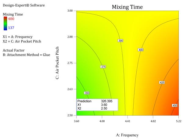
Since the Glue attachment method gives lower mixing times at an Air Pocket Pitch of 2.5 mm, this is the best possible response achieved in the design space. Hence the best response is achieved when Air Pocket Pitch =2.5 mm, Mid-frequency = 3.6 and Attachment Method = Glue. The design space with the optimal solution at a mixing time of 326 seconds (5.4 mins) is shown in Figure 7.

FIGURE 7.

Optimized Mixing time

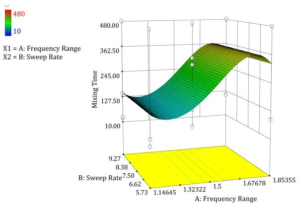
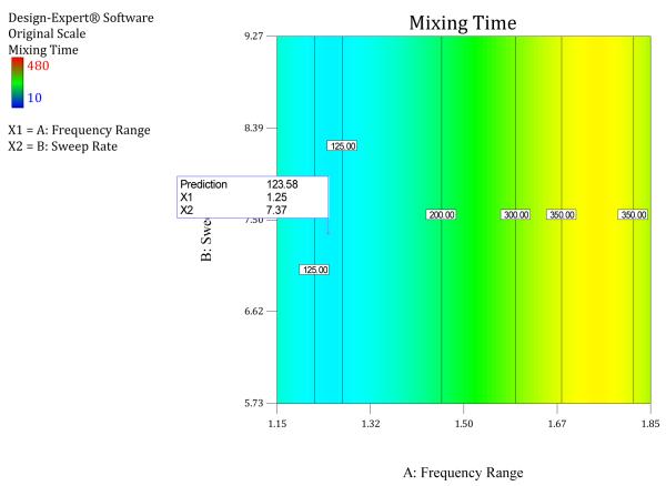
At this stage all parameters with respect to the cartridge dimensions are finalized and so is the mid-frequency where the mixing time is minimized. Now all the cartridge parameters are kept constant and only the frequency range and sweep rate are varied to understand the effect of these two factors on the response (Experiment #5). Five cartridges with 15 chambers each were run to study the effect of these two factors on the response. The ANOVA indicates that only the frequency range affects the response. The 3D Surface plot shown in Figure 8 shows that there is a non-linear relation between the frequency range and the response. The contour plot in Figure 9 shows that the optimum mixing time is obtained when frequency range is 1.25 KHz and any value of sweep rate between 5.73 and 9.27 seconds.

FIGURE 8.

3D surface plot of Frequency range and Sweep rate

FIGURE 9.

Optimized Mixing time

7. CONCLUSIONS

The regression analysis and designed experiments helped the experimenters arrive at an optimal set of levels for all the controllable factors and reduce the effect of the noise on the mixing time. The ridge regression analysis was used to identify factors and the range of these factors. The equation arrived at the end of the regression analysis was not used to predict the response but was used as a baseline to start the sequential designed experiments. The experimentation was done in two groups one with cartridge variables and another with PZT / experimental variables. The strategy of sequential experimentation was followed because the system was known to have a significant amount of noise. Running one large experiment with all the factors would have led to a large amount of noise compared to the signal and would not have led to useful conclusions. To avoid such a situation, the more noisy set of variables were first experimented with and then the PZT variables along with their interactions with the first group of variables were studied.

The final levels of all the controllable factors are given in Table 8. These levels reduce the mixing time to 123.58 seconds.

TABLE 8.

Final Variable settings

Cartridge Manufacturing Variables
No. of air pockets per chamber	21
Piezo offset (distance from PZT to bottom of air pocket)	1 mm
Machine used	Roland
Material used	Polycarbonate

Cartridge Dimension Variables
Diameter of the chamber	13 mm
Depth of chamber	0.60 mm
Depth of air pockets	0.4 mm
Pitch of the air pockets (center line to center line)	2.5 mm

PZT Variables
Diameter of PZT	23.5 mm
Condition of PZT	Double – sided (new)
Attachment method of PZT to cartridge	Glue to bottom of PZT
Frequency Range	1.25 KHz
Sweep Rate	Any value between 5.73 and 9.27 seconds

Experimental Variables
Cartridge position	Vertical
Frequency (static vs. sweep)	Sweep
Rate of sweep	5 seconds
Voltage supplied	20

8. FUTURE PLANS

The fabrication of effective microfluidic components that can be integrated into automated biochemical micro-reactors suitable for practical processing and manipulating small volumes of body fluids remains challenging. However, tremendous advances have been realized with the development of highly sensitive on chip assays for single cell analysis and/or single molecule detection from complex biological mixtures. These advances will open up applications in biomedical and clinical research settings when low cost microfabricated devices would be scaled up for mass fabrication. Polymer injection molding is a low cost fabrication method for disposable microfluidic devices that will require new process quality monitoring but also optimizing design of the molded parts. Regression analysis and rigorous design of experiments will provide paths to understand and identify the important parameters to evaluate the critical performances of the desired microfluidic device produced for a specific biological application and FDA regulatory compliance. For this purpose, FDA pre-IDE filing has been initiated for the microfabricated biodosimeter that will exploit some of the statistical - procedures described above.

REFERENCES

- Elder SA. Cavitation Microstreaming. The Journal of the Acoustical Society of America. 1959;31(1) [Google Scholar]
- Hall EJ, Brenner DJ. Cancer risks from diagnostic radiology. Br. J. Radiol. 2008;81:362–378. doi: 10.1259/bjr/01948454. [DOI] [PubMed] [Google Scholar]
- Xie J, Attinger D. Control and ultrasonic actuation of a gas-liquid interface in a microfluidic chip. Journal of Micromech. Microeng. 2007;II:609–616. [Google Scholar]
- Kolb J, Nyborg WL. Small-Scale Acoustic streaming in liquids. The Journal of the Acoustical Society of America. 1956;28(6) [Google Scholar]
- Lee SY, Ko B, Yang W. Theoretical modeling, experiments and optimization of piezoelectric multimorph. Smart Materials and Structures. 2005;14:1343–1352. [Google Scholar]
- Liu RH, Lenigk R, Grodzinski P. Acoustic micromixer for enhancement of DNA biochip systems. Journal of Microlithography, Microfabrication and Microsystems. 2003;2(3) [Google Scholar]
- Liu RH, Yang J, Pindera MZ, Athavale M, Grodzinski P. Acoustic microstreaming for biological sample mixing enhancement. 2nd Annual International IEEE-EMBS Special topic conference on Microtechnologies in Medicine and Biology; Madison, Wisconsin. May 2-4.2002. [Google Scholar]
- Martel R, Botros I, Rounseville M, et al. Multiplexed screening assay for mRNA combining nuclease protection with luminescent array detection. Assay and Drug Development Technologies. 2002;1(1-1):61–71. doi: 10.1089/154065802761001310. [DOI] [PubMed] [Google Scholar]
- Montgomery DC. Design and Analysis of Experiments. Wiley; New York: 2005. [Google Scholar]
- Montgomery DC, Peck EA, Vining GG. Introduction to Linear Regression Analysis. Wiley; New York: 2006. [Google Scholar]
- Myers RH, Montgomery DC. Response Surface Methodology. Wiley; New York: 2002. [Google Scholar]
- Paul S, Amundson SA. Development of gene expression signatures for practical radiation biodosimetry. Int J Radiat Onc Biol Phys. 2008;741(4):p1236–1244. doi: 10.1016/j.ijrobp.2008.03.043. [DOI] [PMC free article] [PubMed] [Google Scholar]
- Willard GW. Vibrating Liquid Surfaces as generators of Bubbles and Drops. The Journal of the Acoustical Society of America. 1954;26(5) [Google Scholar]
- Yang Z, Goto H, Matsumoto M, Maeda R. Active micromixer for microfluidic systems using lead-zirconate-titanate (PZT)-generated ultrasonic vibration. Electrophoresis. 2000;21:116–119. doi: 10.1002/(SICI)1522-2683(20000101)21:1<116::AID-ELPS116>3.0.CO;2-Y. [DOI] [PubMed] [Google Scholar]
- Yu H, Kwon JW, Kim ES. Microfluidic mixer and transporter based on PZT self-focusing acoustic transducers. Journal of Micromechanical Systems. 2006;15(4) [Google Scholar]
- Sadler D, Zenhausern F. Piezoelectric Mixing Method. 6,986,601 United States Patent.
- Liu R, Lenigk R, Grodzinski P, Zenhausern F. Acoustic micromixer for enhancement of DNA biochip systems. J. Microlithogr. Microfabrication, Microsyst. 2003;2(178) [Google Scholar]