Clustering and Variance Maps For Cryo-electron Tomography Using Wedge-Masked Differences

Abstract

Cryo-electron tomography provides 3D imaging of frozen hydrated biological samples with nanometer resolution. Reconstructed volumes suffer from low signal-to-noise-ratio (SNR)¹ and artifacts caused by systematically missing tomographic data. Both problems can be overcome by combining multiple subvolumes with varying orientations, assuming they contain identical structures. Clustering (unsupervised classification) is required to ensure or verify population homogeneity, but this process is complicated by the problems of poor SNR and missing data, the factors that led to consideration of multiple subvolumes in the first place. Here, we describe a new approach to clustering and variance mapping in the face of these difficulties. The combined subvolume is taken as an estimate of the true subvolume, and the effect of missing data is computed for individual subvolumes. Clustering and variance mapping then proceed based on differences between expected and observed subvolumes. We show that this new method is faster and more accurate than two current, widely used techniques.

1. Introduction

1.1. Background

Cryo-electron tomography provides 3D imaging of biological structures in their native conformation with nanometer resolution (Frank, 2006; Hoenger and McIntosh, 2009). The unstained, unfixed samples are highly susceptible to beam damage, however, necessitating the use of low dose imaging, and resulting in low signal-to-noise ratio (SNR) images. Significant artifacts caused by incomplete sampling of Fourier space are also typically present. If the reconstructed volume contains multiple, identical copies of a structure of interest in varying orientations, both problems can be overcome by alignment and weighted averaging of extracted subvolumes in Fourier space. PEET (Nicastro et al. (2006); Cope et al. (2010), http://bio3d.colorado.edu/PEET) is an open source package which performs such alignment and averaging.

Averaging implicitly assumes identical particles. This assumption must be checked using clustering (unsupervised classification) prior to, during, or after averaging. Prior clustering of 2D projections to provide homogeneous subclasses for reconstruction is common in single particle techniques (Frank, 2006; Bartesaghi et al., 2008). Recently, Scheres et al. (2007, 2009) described a 3D method based on the expectation-maximization (EM) algorithm (Dempster et al., 1977) in which alignment, estimation of missing data, classification and reconstruction of class averages proceed simultaneously. Yu et al. (2010) also utilize expectation-maximization after alignment in their PPCA-EM algorithm to estimate missing data and to extract features for clustering. In section 2.1 below we describe a new technique for clustering after averaging. Hybrid or iterative application of these methods is also possible, and may be required in difficult cases.

Clustering requires choosing a particular algorithm as well as the feature or features to which the algorithm will be applied. Numerous clustering algorithms with varying strengths and weaknesses are well known (e.g. see Bishop (1995), Duda et al. (2001) and Frank (2006)). While some, e.g. auto-associative multilayer neural networks, contain built-in dimensionality reduction, most require explicit dimensionality reduction before application to very high-dimensional data such as 3D tomographic volumes.

Dimensionality reduction is often accomplished using one of several closely related techniques based on eigendecomposition. Historically, correspondence analysis was the first of these techniques applied to electron microscopy (van Heel and Frank, 1981; Bretaudiere and Frank, 1986). Correspondence analysis requires non-negative values, however, and is therefore not strictly applicable to either tomographic volumes or cross-correlations, both of which can be negative. Singular value decomposition (SVD), either of a cross-correlation or other symmetric similarity (or dissimilarity) matrix or of a covariance matrix is now widely used for this purpose, e.g. see Frank (2006). SVD of a covariance or correlation matrix is also known as principal component analysis (PCA). Following Förster et al. (2008) it has become common in the electron microscopy literature to also refer to SVD of a cross-correlation matrix as PCA². We consider this terminology unfortunate, since the two approaches result in slightly different behavior. In the following, we will distinguish between them, using the terms “PCA” and “SVD of a cross-correlation”, respectively.

Clustering of tomographic subvolumes using uncorrected cross-correlation or covariance matrices often fails badly, with artifacts due to missing tomographic data obscuring any real variation. Approaches to dealing with this issue include restricting the computation to include only the non-missing data (Bartesaghi et al., 2007, 2008; Förster et al., 2008), imputing or otherwise filling in the missing data (Scheres et al., 2007, 2009; Yu et al., 2010), and applying ad hoc corrections to the cross-correlation or covariance (Schmid and Booth, 2008). Schmid and Booth (2008) noted that cross-correlation between otherwise identical subvolumes falls off approximately in proportion to the fractional overlap between their shared informative (i.e. non-missing) regions in Fourier space and suggested rescaling by the inverse of this factor. PEET has used such rescaling since its initial implementation by Nicastro et al. (2006). Förster et al. (2008) and Bartesaghi et al. (2007, 2008) restrict computation of the similarity or dissimilarity metric to the mutually shared informative region. When the metric in question is cross-correlation, this approach has come to be known as “constrained cross-correlation”. We will refer to clustering based on eigendecomposition of these corrected metrics as “SVD of a rescaled cross-correlation” (SVD-RCC) and “SVD of a constrained cross-correlation” (SVD-CCC), respectively. Singular value decomposition (Golub and van Loan, 1996) plays a key role in understanding the algorithms described here, as well as a robust and convenient computational module for their implementation. Because it may not be familiar to some readers, we provide a brief introduction to SVD in section 6.1 of the supplemental data.

In this report, we describe a new approach based on what we call “wedge-masked differences” (WMDs). Originally developed as a correction to covariance, this method is applicable to cross-correlation as well and also leads naturally to a framework for constructing variance maps. Liu and Frank (1995) and Penczek et al. (2006) have discussed the issues associated with 3D variance estimation and analysis in the context of single-particle reconstruction. Variance estimation in cryo-tomography is somewhat simpler, due to the availability of independent reconstructions for each subvolume. As shown below, the proposed correction substantially reduces the impact of missing data on the resulting estimates.

2. Theory

2.1. Wedge-Masked Differences

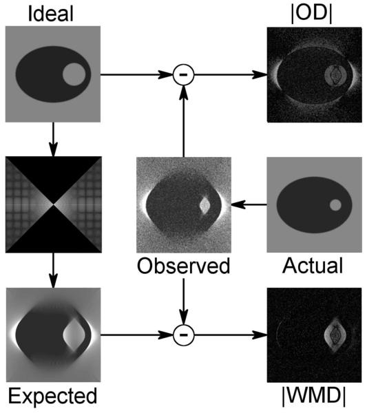
Figure 1 presents a conceptual illustration of the problem at hand as well as our proposed solution. Panels in this figure can be thought of, loosely, as sections through cylindrical volumes. Conventional PCA and variance mapping are based on the magnitudes of the ordinary differences (ODs) between the ideal (or estimated) object and the corresponding, aligned reconstructions of single particles. ODs are highly susceptible to artifacts from systematically missing data, as illustrated. If we know which data are missing, however, we can compute an expected volume for each particle. WMDs, which are differences between the expected and observed subvolumes, largely suppress missing data artifacts while preserving genuine variations. In single tilt-axis tomography, the required missing data region locations are completely defined by the tilt series acquisition geometry and the Euler angles which are estimated during alignment.

Figure 1.

Comparison of wedge-masked and ordinary differences. Ideal: The ideal or true object. If not known, the ideal may be well approximated by weighted averaging or other techniques. Actual: An individual, sample object containing a smaller hole than the ideal. Individual objects are typically not accessible to direct observation. Instead, we have access only to Observed: a tomographic reconstruction of the actual object suffering from noise and missing data artifacts. |OD|: Magnitude of the ordinary difference between the ideal and observed objects. In addition to the real variation in hole diameter, ODs are heavily influenced by missing data artifacts, resulting in a bright halo. If parameters defining the missing data are known or have been estimated, they can be applied to compute an Expected object from the ideal. In this particular example, we Fourier transform the ideal, zero out a vertically oriented 90° missing wedge, and then invert the masked Fourier transform. |WMD|: Magnitude of the “wedge-masked” difference between the expected and observed objects. WMDs preserves true variation while largely suppressing missing data artifacts.

In overview then, we proceed as follows. Taking the averaged subvolume as an estimate of the true subvolume, the effect of missing data is computed for each aligned particle yielding an expected subvolume. Clustering and variance mapping then follow based on the covariance of the differences between expected and observed subvolumes.

Formally, assume we have an “average” volume x* containing m voxels with 3D Fourier transform ℱ(x*) = X*, resulting from aligning and weighted, Fourier space averaging of 1 ≤ i ≤ n particles or subvolumes, x_i, drawn from among l tomograms, where 1 ≤ v_i ≤ l indicates the tomogram from which the ith particle was sampled, with m ⪢ n. The jth tomogram has an associated “wedge mask”, W_j, a binary Fourier domain mask with zeros and ones indicating the missing and informative tomographic regions, respectively, in reciprocal space tomogram coordinates. The term “wedge mask” derives from the fact that the missing region is wedge-shaped in single tilt axis tomography. The mask need not be wedge shaped, however, and any systematically missing regions in reciprocal or real space can be accommodated. Finally, let parameters θ_i specify the alignment (rotation and translation) found for the ith particle, with R_θi denoting the matrix required to rotate the ith particle to its aligned orientation.

If sufficient particles with varying orientations have contributed to the average, x* will be relatively free of both noise and missing tomographic data artifacts compared to the individual volumes. Assuming a homogeneous population and correct subvolume alignment, we treat x* as an estimate of the true subvolume of interest. Since alignment parameters, and specifically rotations, have been estimated for each subvolume, we can compute the expected subvolume for each particle by applying an appropriately rotated wedge mask to x*. Differences between expected and observed subvolumes are then used to highlight unexpected variation and to check the assumption of population homogeneity, as outlined in Table 1.

Table 1.

WMD-corrected PCA and Variance Mapping.

Initialize an m by n matrix D = [0] For each particle, i – Construct the rotated wedge mask: $$W^{\prime }=C{\mathbf{R}}_{{\theta }_i}\left(W_{v_i}\right)$$ – Apply the wedge mask to the subvolume and average, and band limit the subvolume: $$\begin{array}{c}\hfill t={\mathcal{F}}^{-1}\left(W^{\prime }{X}^{\ast }\right)\hfill \\ \hfill y={\mathcal{F}}^{-1}\left({\mathit{BW}}^{\prime }{X}_i\right)\hfill \end{array}$$ – Form the wedge-masked difference: δ = t − y – Apply an ROI mask, if any: δ = pδ – Centralize or standardize as desired. In most of the work described here, we adjusted δ to be zero mean and unit variance over p, and zero elsewhere. More recently, we have stopped adjusting variance. – Set column i of D to δ: [di] = δ Center the columns of D: ${\mathbf{d}}_i={\mathbf{d}}_i-\frac{1}{n}{\displaystyle {\Sigma }_{i=1}^n}{\mathbf{d}}_i$ Compute the [partial] SVD of the WMDs: USVT = D Cluster using first k rows of SVT as inputs to the chosen algorithm If desired, form the corrected covariance: C = US2UT/(n − 1) and the variance map σ2 = diag(C)

In Table 1 and the following, we sometimes treat volumes as 1D column vectors, with elements presented in a predefined, canonical order. (The order chosen does not matter, so long as it is applied consistently). In most cases, the distinction between a volume and vector will be apparent from the context. To avoid possible confusion, however, vectors are explicitly denoted using lower case bold font. Thus x and x refer to the same data, treated as a 3D volume or as a 1D vector respectively. Similarly, matrices are denoted with upper case bold font, and the ith column of matrix M as m_i.

To improve noise rejection, we allow use of an optional bandpass filter with Fourier representation B to be applied to individual volumes. Additionally, a spherical low pass filter C with a Gaussian rolloff starting at 0.4827 times the sampling frequency and with a standard deviation of 0.025 is always applied to the rotated wedge mask. These parameters are chosen to provide an amplitude response of 0.5 at the Nyquist frequency, reducing the impact of frequencies in the corners of cubical regions in Fourier space. Unlike the user-defined bandpass, this minimal filter is applied to both individual subvolumes and the average.

It is sometimes desirable to focus attention on specific subregions of interest. To this end, we also allow an object space binary particle mask, p, with zeros and ones indicating the regions to be ignored and considered during clustering, respectively.

Following the algorithm in Table 1, we form a matrix of centered, wedge-masked differences and decompose it using SVD. We thus have expressed the WMDs in terms of eigenvectors, given by the columns, u_i, of U, and with coefficients given by the columns of SV^T.

For clustering, only coefficients along the first few eigenvectors are needed, rather than the complete decomposition. These coefficients are used as input to the chosen clustering algorithm. This is readily accomplished by using only the first k columns of U as basis vectors, and the first k rows of SV^T as coefficients. Since only the k largest eigenvectors and singular values are needed, the complete SVD is not required. Packages such as ARPACK to perform such computations efficiently are available (Lehoucq et al. (1998), http://www.caam.rice.edu/software/ARPACK/). Note also that the eigenvectors of the WMD-corrected covariance matrix and the associated coefficients are calculated without explicit evaluation of the covariance matrix. This makes the present method more computationally efficient than either rescaled or constrained cross-correlation. In each of those algorithms the form of the correction used forces explicit evaluation of the corrected cross-correlation matrix prior to calculation of the SVD.

Variance mapping can be useful in significance testing and in identifying both conserved and variable regions in the 3D average, with highly variable “hot spots” identifying potential candidates for masking. As was the case with covariance and cross-correlation, an uncorrected variance map is of little use, because it is corrupted and typically dominated by artifacts due to missing data. Fortunately, the same WMD correction used for PCA also yields corrected covariance and variance. As indicated in Table 1, the WMD-corrected covariance matrix is given by C = US²U^T / (n − 1). The corrected variance map is just the diagonal of C, σ² = diag(C), where σ² should be interpreted as a 3D volume with voxels in one-to-one correspondence with those of the average, x*. Standardization of the WMDs should typically be omitted during variance mapping, since it could cause a change of scale. While the complete SVD is typically desirable, full evaluation of the covariance matrix is not needed, since only the diagonal elements are of interest.

2.2. Extensions to Wedge-Masked Differences

In some cases, additive offsets or differences in amplitude may be present between subvolumes or between the “average” and individual subvolumes (e.g. if the average results from modeling or a different imaging modality). Additive offsets can be handled by adjusting both wedge-masked and average subvolumes to be zero mean, or by adjusting individual wedge-masked subvolumes to match the mean of the corresponding wedge-masked average.

Multiplicative gain differences are only slightly more problematic. Because individual subvolumes can have SNR much less than 1, a simple wedge-masked difference between observed and expected subvolumes could result in a noisy, possibly contrast-reversed copy of the masked average when differences in signal amplitude are present. To avoid such problems, each WMD can be computed as the difference between the masked average and a multiple of the masked subvolume, with the multiplier chosen to yield the minimum norm difference for each subvolume. Specifically, in Table 1, one would replace the ordinary WMD, δ = t − y, with the minimum norm WMD, δ = t − (t · y/|y|²) y. Since the data sets used here do not suffer from significant offsets or gain differences, we use simple WMDs in the following.

3. Methods

To compare performance of WMD-corrected PCA with that of SVD of rescaled or constrained cross-correlation, we used a semi-synthetic data set based on the 4 binary variants of the Yarrowia lipolytica complex I created by Yu et al. (2010) for evaluating their PPCA-EM algorithm. The 4 initial volumes, provided by them, consist of the original and 3 intentionally distorted versions, each with 160³ 3.6 Å voxels. Volume 1 contains the original, while volumes 2–4 have been distorted using the skew transformation:

$$\left(\begin{array}{c}\hfill x^{\prime }\hfill \\ \hfill y^{\prime }\hfill \\ \hfill z^{\prime }\hfill \end{array}\right)=\left(\begin{array}{ccc}\hfill 1\hfill & \hfill a\hfill & \hfill b\hfill \\ \hfill 0\hfill & \hfill 1\hfill & \hfill c\hfill \\ \hfill 0\hfill & \hfill 0\hfill & \hfill 1\hfill \end{array}\right)\left(\begin{array}{c}\hfill x\hfill \\ \hfill y\hfill \\ \hfill z\hfill \end{array}\right)$$

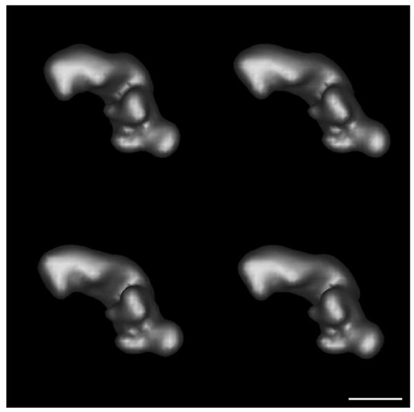
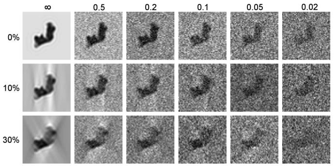
with (a, b, c) = (0.25, 0.1, 0.1), (0.1, 0.25, 0.1), and (0.1, 0.1, 0.25), respectively. For purposes of this study, these initial volumes were low pass filtered to an amplitude response of 0.5 at 3 nm using a Gaussian filter with a standard deviation of 0.02 commencing at 0.096452 inverse voxels. The low pass filtered volumes were decimated 2.5X and padded to a final final size of 96³ 9 Å voxels. Isosurface representations of these decimated, low pass filtered volumes are shown in Figure 2. 100 copies of each volume in arbitrary orientations were created with uniform random rotations generated using the algorithm of Shoemake (1992). The resulting population of 400 noise-free, simulated volumes with no missing tomographic data was aligned using PEET, and the resulting alignment parameters used repeatedly for averaging and clustering the 400 volumes with varying amounts of added Gaussian noise and missing tomographic data. SNRs from ∞ to 0.02 were explored, with SNR specified as a ratio of particle to noise variance, and with particle variance estimated over the central 1/8th of the volume (1/2 of each linear dimension). Similarly, single axis missing wedges comprising from 0 to 30% of the tomographic volume were simulated, the latter corresponding to a tomographic tilt range from −63° to 63°. Figure 3 shows a sample 9 Å xy cross sections through volume 1, illustrating the impact of noise and missing tomgraphic data over the range tested.

Figure 2.

The 4 test volumes. Undistorted complex I (volume 1) is at the upper left, with volumes 2–4 proceeding clockwise. Volumes 2–4 have been distorted with a skew transform

$$\left(\begin{array}{c}\hfill x^{\prime }\hfill \\ \hfill y^{\prime }\hfill \\ \hfill z^{\prime }\hfill \end{array}\right)=\left(\begin{array}{ccc}\hfill 1\hfill & \hfill a\hfill & \hfill b\hfill \\ \hfill 0\hfill & \hfill 1\hfill & \hfill c\hfill \\ \hfill 0\hfill & \hfill 0\hfill & \hfill 1\hfill \end{array}\right)\left(\begin{array}{c}\hfill x\hfill \\ \hfill y\hfill \\ \hfill z\hfill \end{array}\right)$$

with (a, b, c) = (0.25, 0.1, 0.1), (0.1, 0.25, 0.1), and (0.1, 0.1, 0.25), respectively. With the exception of volume 2, whose long axis is noticeably stretched, the resulting distortions are quite subtle, providing a stringent test for clustering. Scale bar is 10 nm.

Figure 3.

Central 9 Å xy cross-sections of volume 1 showing the impact of noise and single-axis missing tomographic data. Top: no missing data; Middle: 10% missing (tilt range −81° to 81°); Bottom: 30% missing (tilt range −63° to 63°). SNR is ∞, 0.5, 0.2, 0.1, 0.05, and 0.02, from left to right, respectively. For purposes of illustration, z was used as the tilt axis, and the brightness and contrast of each image was adjusted individually.

A spherical particle mask with a radius of 25 voxels was used, as was a low pass filter with Gaussian rolloff commencing at 0.25 with a standard deviation of 0.05 inverse voxels. Plots of singular values and histograms of the corresponding coefficients were used to select specific coefficients to consider for clustering, which was accomplished using k-means with 10-fold replication and selection of the best clustering score to minimize sensitivity to initial seeds. Model complexity (i.e. the number of clusters) was chosen, and significance of resulting fits judged using Akiake (AIC) and Bayes (BIC) information criteria (Hastie et al., 2002).

To compare the performance of uncorrected and WMD-corrected variance maps, a 200 particle subset of the test data containing only volumes 1 and 2 was used with 30% missing data and an SNR of 0.2. The weighted average, uncorrected, and corrected variance maps were computed, and the resulting variance maps compared to the squared differences between the original, noise-free volume with no missing data.

All of the experiments with semi-synthetic data use an alignment based on noise-free volumes with no missing data. This provides a fair comparison between the various corrections, but also leads to optimistic performance estimates. In real applications alignment would also be impaired by noise and missing data, and performance would be expected to fall off more quickly than shown here.

Performance of clustering and variance mapping using WMDs was also evaluated on experimental data sets. Clustering was performed on GroEL₁₄ / GroEL₁₄GroES₇ tomographic data similar to those previously described by Förster et al. (2008) and provided by them. 786 pre-aligned subvolumes, each containing 32³ 12.0 Å voxels were analyzed. The first 214 subvolumes were reconstructed from a tiltseries containing only GroEL₁₄, while the remaining 592 were from a tiltseries containing a mixture of GroEL₁₄ and GroEL₁₄GroES₇ particles, along with damaged or incomplete particles.

WMD-corrected variance mapping was performed on averaged microtubule doublets from Chlamydomonas reinhardtii wild type axonemes (Heuser et al., 2009). 652 subvolumes selected with 96 nm periodicity along microtubule doublets were aligned and averaged with PEET, and the WMD-corrected variance map computed as described in Table 1.

Code incorporating WMD-PCA, SVD-RCC, and SVD-CCC into PEET was written in MATLAB® (The MathWorks, Natick, MA) and is available for download at http://bio3d.colorado.edu/PEET.

4. Results

4.1. Clustering With No Missing Data

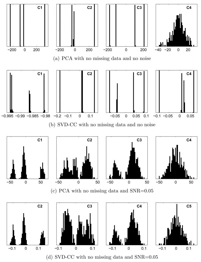
In the absence of missing data, all 3 corrections described above become irrelevant. WMD-PCA reduces to standard PCA, and SVD-CCC and SVD-RCC reduce to SVD of cross-correlation (SVD-CC). Not surprisingly, when noise is also absent, both techniques perform exceptionally well on the test data. Using PCA, the first 3 eigenvectors account for 44.7%, 29.6%, and 24.8% of the overall variance, respectively, for a total of 99.1%. As illustrated in Figure 4(a), histograms of the coefficients along these vectors are highly structured, with clearly separated, discrete peaks. These turn out to correspond to individual classes, and k-means using any of these features alone or in combination results in perfect clustering of all 400 subvolumes. Histograms of subsequent coefficients, only one of which is shown, become progressively narrower and more Gaussian.

Figure 4.

Coefficient histograms with no missing data. (a),(b): SNR=∞. (c), (d): SNR=0.05. In (a) and (b), discrete peaks correspond to individual classes. In (c) and (d), the 3 peaks in the left panel correspond to classes 1, 3+4 (combined), and 2. Subsequent coefficients provide further resolution.

SVD-CC also performs perfectly in this idealized case, as illustrated in Figure 4(b). The first 4 coefficients are all highly structured. Features 2–4 in isolation each result in perfect clustering, while Feature 1 alone misclassifies only a single volume using k-means. Unlike in PCA, eigenvalues are no longer proportional to the fraction of variation explained, so slightly more care is required in interpretation and in choosing features. Coefficients along the first eigenvector are typically offset from 0, reflecting the non-zero mean correlation. The square of this offset adds to the first eigenvalue, inflating its size, while contributing no information useful for clustering. Compensation by subtracting the mean squared coefficient value is possible, but we take the more direct approach of simply examining histograms for both width and structure. Note in Figure 4(b) that while coefficient 1 does contain useful structure, its distribution is substantially narrower, and therefore more susceptible to noise, than those of the following coefficients. Hereafter, coefficient 1 histograms for SVD-RCC and SVD-CCC will be displayed only when their contribution to clustering is significant.

The effect of adding Gaussian noise to an SNR of 0.05, still with no missing data, is shown in Figures 4(c) and 4(d). The most informative coefficient (1 for PCA, 2 for SVD-CC), still separates classes 1 and 2 perfectly, while classes 3 and 4 are no longer resolved. Including the next 2 coefficients restores perfect clustering in both cases, as does using the first and third coefficients (1 and 3 for PCA, 2 and 4 for SVD-CC). Using only the first 2 coefficients, results in nearly perfect clustering with minor overlap between classes 3 and 4.

Gaussian noise at an SNR of 0.02 yields only slightly poorer results (not shown), with the leading coefficient giving nearly perfect 3-class separation, and the leading 3 coefficients giving nearly perfect 4-class separation for both PCA and SVD-CC.

4.2. Clustering With Missing Data

With missing tomographic data, the 3 corrections become distinct and must be analyzed separately. Several common trends become apparent, however. With increasing missing data and with decreasing SNR, formerly discrete peaks broaden and eventually become indistinct. Simultaneously, coefficient distributions become less structured and their widths more uniform, making it harder to identify potential features for clustering.

SVD-RCC is the first technique to fail as the amount of missing data increases. With just 10% missing data and no added noise, the distributions of the leading coefficients become largely structureless, as shown in Supplemental Figure S1 in the online version. The leading 4 coefficients still result in good, but not perfect separation of class 1 from the other classes. (Coefficients 2–7 jointly do lead to perfect 2-class clustering, but this grouping does not appear significant using AIC and BIC, and is unlikely to be detected in real applications). SVD-CCC and WMD-PCA still perform very well under these conditions. In both cases, the leading 3 coefficients alone (2–4 for SVD-CCC, 1–3 for WMD-PCA) yield perfect clustering. Additionally, in each case the leading, single coefficient gives perfect 3-class clustering, with classes 1 and 2 distinct, but classes 3 and 4 lumped together.

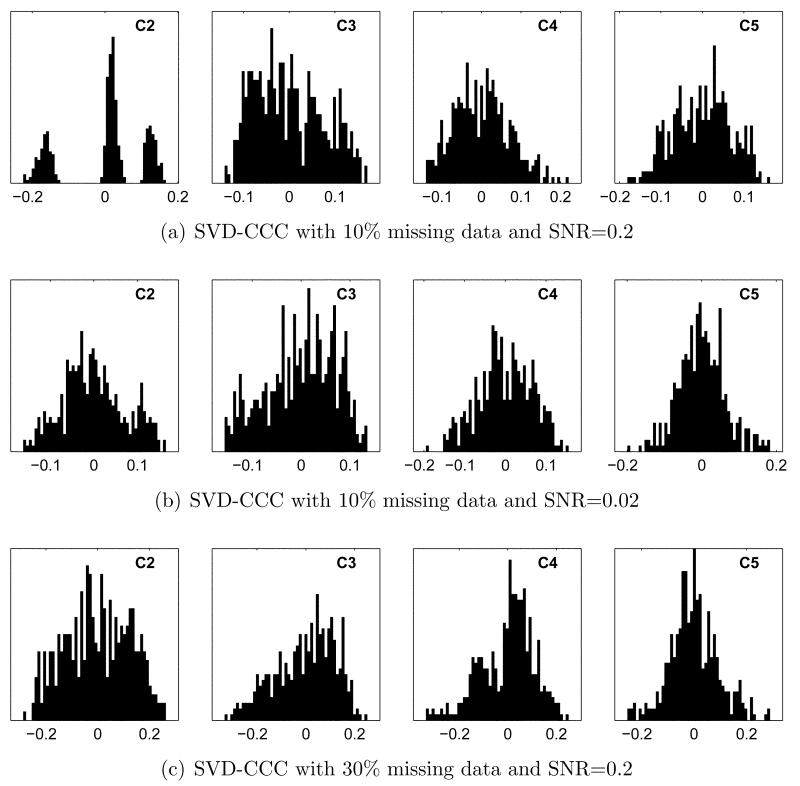
Sample distributions illustrating the performance of SVD-CCC with increasing noise and missing data are shown in Figure 5. With 10% missing data and and SNR of 0.2 (Figure 5(a)), classes 3 and 4 are no longer resolved, but coefficient 2 still yields perfect 3-class separation. At an SNR of 0.02, some structure remains, as shown in Figure 5(b), resulting in 2-class separation using the leading 4 coefficients. With 30% missing data and an SNR of 0.2 (Figure 5(c)), clustering is unsuccessful.

Figure 5.

Coefficient histograms for SVD-CCC with missing data and noise. (a, b): 10% missing data, SNR 0.2 and 0.02, respectively. (c): 30% missing data, SNR 0.2. In (a), coefficient 2 yields perfect 3-class separation. Clustering using k-means gives only 2-class separation in (b) and fails to find any significant clusters in (c).

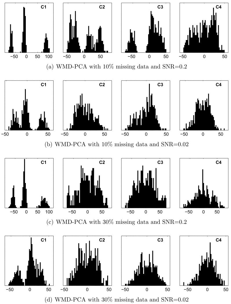
Of the 3 corrections tested, WMD-PCA proved most resistant to missing data and noise, as illustrated in Figure 6. With 10% missing data, coefficients 1–3 lead to perfect clustering out to and including³ an SNR of 0.05. Coefficient histograms at an SNR of 0.2 are shown in Figure 6(a) for comparison with the corresponding results in Figure 5(a). Similarly, coefficient 1 alone yields perfect 3-class separation out to an SNR of 0.05 and good separation at an SNR of 0.02 (Figure 6(b)). With 30% missing data, coefficients 1–4 give very good 4-class separation out to an SNR of 0.05. At an SNR of 0.2, where SVD-CCC fails, coefficient 1 alone gives perfect 3-class separation (Figure 6(c)). Perfect separation is attainable using more features: coefficients 1-5 suffice out to an SNR of 0.1, while coefficients 1–8 are required at an SNR of 0.05. Finally, at an SNR of 0.02 much of the structure in the coefficient histograms is lost, as shown in Figure 6(d). Even in this case, coefficient 1 alone gives very good, although not perfect, separation of class 1 from the remaining 3 classes. In all cases, the resulting groupings were judged highly significant by both AIC and BIC.

Figure 6.

Coefficient histograms for WMD-PCA with missing data and noise. (a, b): 10% missing data, SNR 0.2 and 0.02, respectively. (c, d): 30% missing data, SNR 0.2 and 0.02, respectively. Panels (a)–(c) are directly comparable to Figure 5(a)–5(c) for SVD-CCC, and show that WMD-PCA better preserves separation between classes.

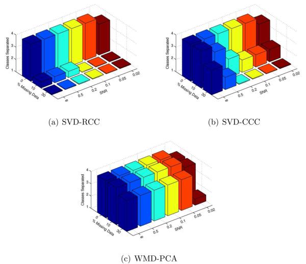
Figure 7 summarizes the number of classes successfully separated by k-means clustering on the leading 4 coefficients for each method over a wide range of conditions. In this figure, we have adopted the convention that perfect 3-class separation, for example, is shown with a bar height of 3, while good, but not perfect, 3-class separation is shown with a bar height of 2.5. As illustrated, WMD-PCA discriminates successfully between classes with more noise and missing data than either SVD-RCC or SVD-CCC.

Figure 7.

Number of classes separated using k-means on the leading 4 coefficients. A bar height of N indicates perfect N-class separation, while a height of N − 0.5 indicates good, but not perfect separation. WMD-PCA outperforms both other methods in the presence of noise and missing data.

4.3. Eigenvolumes and Variance Mapping

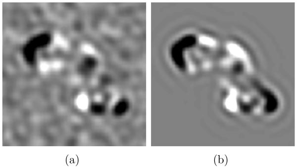
Another advantage of PCA over SVD of cross-correlation is that each eigenvector is directly interpretable as a change (eigenvolume or eigenimage) from the average volume. Figure 8(a) shows a central 5.4 nm thick xy slice through WMD-PCA eigenvector 1 with 30% missing data and an SNR of 0.02. The result corresponds nicely with a similar slice through the true difference between classes 1 and 2, shown in Figure 8(b), accounting for the good 2-class separation achieved even under these fairly extreme conditions.

Figure 8.

Central 5.4 nm xy slices through (a): WMD-PCA eigenvector 1 with 30% missing data and SNR= 0.02, and (b): the exact difference between volumes 1 and 2 with no noise and no missing data.

As described above, the WMD correction can also be applied to generate a map of the variance (or its square root, the standard deviation) partially corrected for artifacts caused by missing tomographic data.

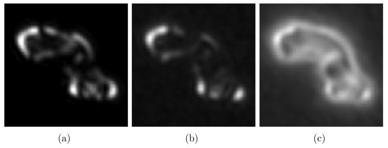
Figure 9 shows central 5.4 nm xy slices through the true, WMD-corrected, and uncorrected standard deviation maps. The latter 2 were constructed using 100 randomly oriented particles each from classes 1 and 2 with 30% missing data and an SNR of 0.2. True standard deviation was calculated as the square root of 0.175 times the squared differences between classes 1 and 2. The factor of 0.175 is the product of a factor of 0.5² to compensate for the use of class differences rather than differences from the mean and a factor 0.7 to simulate missing wedge attenuation. While the uncorrected map contains numerous artifacts resulting from the missing tomographic wedge, the WMD-corrected map eliminates most of these artifacts and more closely approximates the true standard deviation.

Figure 9.

Central 5.4 nm xy slices of standard deviation maps. (a): true standard deviation between classes 1 and 2, computed as the square root of 0.175 times the squared difference between the volumes. (b,c): WMD-corrected and conventional (uncorrected) estimates, respectively, of standard deviation with 30% missing data and SNR=0.2.

4.4. Throughput and Combining Corrections

With our present MATLAB (R2010b) implementation, WMD-PCA is the fastest of the 3 methods, followed by SVD-RCC, and then SVD-CCC. On a dual 3.33 GHz Xeon 5590 with 72 Gb of RAM, a single WMD-PCA, SVD-RCC, or SVD-CCC decomposition of our 400 particle test set takes approximately 200, 400, and 1400 seconds, respectively.

On the synthetic test data, WMD-PCA is also the most robust of the 3 corrections in the face of systematically missing data and noise, followed by SVD-CCC, and then by SVD-RCC. Since only WMD-PCA utilizes PCA (i.e. SVD of a covariance), while the remaining 2 corrections utilize SVD of a cross-correlation, it is reasonable to question whether the observed difference in accuracy is due to the WMD correction per se, or due to covariance being more robust and informative than cross-correlation. Figure 4 suggests that covariance and cross-correlation are similarly informative with no missing data and no noise. To permit similar comparison in the presence of noise and missing data, we performed the WMD correction, followed by computation of rescaled cross-correlations, and, finally, SVD of the corrected cross-correlation matrix, effectively applying the WMD correction to SVDRCC. The combined algorithm, WMD-SVD-RCC, performs comparably to WMD-PCA under all conditions with missing data (e.g. see Supplemental Figure S2 in the online version), confirming that the WMD correction is responsible for the observed performance differences. As an aside, the WMD correction often, but not always, removes much of the offset present with SVD-RCC, making coefficient 1 informative again. For this reason, coefficient 1 is included in panels (a)–(c), but not (d) of Supplemental Figure S2.

4.5. GroEL and GroEL/GroES Clustering

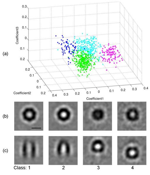
To verify the performance of WMD-PCA clustering on experimental data, we used a GroEL/GroES data set previously described by Förster et al. (2008) and supplied by them. 214 aligned subvolumes containing GroEL₁₄ particles and 572 subvolumes containing a mixture of GroEL₁₄, GroEL₁₄GroES₇, and damaged or incomplete particles were grouped into 4 classes using k-means clustering on the first 3 eigenvectors from WMD-PCA, as show in Figure 10. Of the 214 GroEL₁₄ particles, 201, 4, 2, and 7 were assigned to classes 1–4, respectively. Of the 572 mixed GroEL/GroES particles, 123, 281, 104, and 64 were assigned to classes 1–4, respectively. Based on these results and on similarity between the class averages and previously published structures, we conclude that class 1 corresponds to GroEL₁₄, class 2 to GroEL₁₄GroES₇, and classes 3 and 4 to damaged, incomplete or misaligned particles positioned at the top and bottom of the average particle, respectively. Of the 214 putative GroEL₁₄ particles, 93.9% were thus classified correctly, 1.9% misclassified as belonging to class 2, and 4.2% classified as damaged or misaligned. Similarly, of the 285 particles classified as belonging to class 2, 281 (98.6%) were drawn from the 572 subvolumes containing GroES₇. These results compare favorably with those reported previously (Förster et al., 2008).

Figure 10.

GroEl₁₄/GroEL₁₄GroES₇ clustering using WMD-PCA. (a): k-means clusters using the first 3 eigenvectors. Class 1–4 are shown in green, cyan, magenta, and blue, respectively. (b, c): Central 1.2 nm xy (b) and xz (c) slices through the 4 class averages. Class 1 and 2 averages correspond to GroEl₁₄ and GroEL₁₄GroES₇, respectively, while classes 3 and 4 appear to contain incomplete, damaged, or misaligned particles positioned at the top or bottom of the overall average. Scale bar is 10 nm.

We also performed clustering on these data using our implementation of SVD-RCC and SVD-CCC on the 4 leading eigenvectors. (We note in passing, that these are examples where eigenvector 1 is useful, despite being offset from 0). SVD-CCC yielded results almost identical to those for WMD-PCA, while SVD-RCC performed only slightly worse, misclassifying 14 particles from the GroEL₁₄ subvolumes as belonging to class 2.

4.6. Chlamydomonas Axoneme Variance Mapping

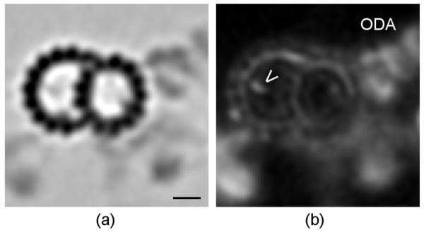
Similarly, we verified WMD-corrected variance mapping performance on Chlamydomonas reinhardtii axoneme data previously described by Heuser et al. (2009) and provided by them. As illustrated in Figure 11, in an axial projection the outer dynein arm and beak regions both show up as areas with high variance, particularly relative to their densities in the average. This is expected from previous studies, since the beak is present in only some doublets, while the outer dynein arms are missing from doublet 1 (Hoops and Witman, 1983). Unexpectedly large variance is also observed in the inner dynein arm region. Variations in this area have only recently been noted and are still under investigation (Nicastro, 2009).

Figure 11.

Chlamydomonas reinhardtii axoneme axial projections. (a): The averaged doublet structure. (b): The WMD-corrected variance map corresponding to (a). The beak (open arrowhead) and outer dynein arm (ODA) regions are indicated. Both show up as regions with high variance relative to their densities in the average, as expected from the known structure. Scale bar is 10 nm.

5. Discussion

The key idea leading to WMD-corrected covariance is hardly novel. Analysis of squared differences between observed and expected (or estimated) values is one of the most basic techniques in statistics. It is therefore somewhat surprising that this simple and seemingly effective correction has gone unnoticed in cryo-tomography for so long. As we have shown above, WMD-corrected covariance is less computationally intensive and, at least on our synthetic test data, more robust against missing data artifacts than rescaled or constrained cross-correlation. We have demonstrated that this improvement in accuracy is due the WMD correction per se, and not to any inherent difference between cross-correlation and covariance.

With hindsight, the improved sensitivity and accuracy provided by the WMD correction is not surprising. Since constrained cross-correlation handily outperforms rescaled cross-correlation (presumably due to better rejection of missing data artifacts), consider only the former. Imagine two subvolumes whose Fourier transforms differ from one another and from the “true” average in their respective informative regions, but not in the mutually shared overlap between these regions. Constrained cross-correlation, indeed any constrained metric computed only over the mutually shared region, is blind to such differences, while WMD-corrected covariance treats them, correctly, as prima facie evidence of population heterogeneity. Constrained metrics thus fail to exploit all of the available information.

While we have presented WMD-corrected covariance in the context of 3D electron tomography, the approach is more general, and is applicable to other fields and to any number of dimensions, so long the data are partially missing in a known and systematically varying fashion.

Two potential limitations of WMD-corrected PCA are that it requires an estimate of the true subvolume, and that, like PCA in general, it lacks an explicitly probabilistic framework. Recent techniques addressing both issues are available. The probabilistic PCA (PPCA) method of Roweis (1998) and Tipping and Bishop (1999) provides a probabilistic framework for PCA and uses the EM algorithm of Dempster et al. (1977) for iterative solution. Yu et al. (2010) have applied this method to the problem at hand in their PPCA-EM algorithm, simultaneously estimating the average volume while extracting coefficients useful for subsequent classification. Scheres et al. (2009) have also proposed a method using the EM algorithm on unaligned data, attempting simultaneous alignment, missing data estimation, classification, and estimation of class averages, with regularization to help avoid local minima. These (and other) techniques vary considerably in their prerequisites, computational intensity, and outputs. Determining which will prove most effective in particular circumstances remains a task of considerable importance.

References

- Bartesaghi A, Sprechmann P, Liu J, Randall G, Sapiro G, Subramaniam S. Classification and 3D averaging with missing wedge correction in biological electron tomography. Journal of Structural Biology. 2008;162:436–450. doi: 10.1016/j.jsb.2008.02.008. [DOI] [PMC free article] [PubMed] [Google Scholar]
- Bartesaghi A, Sprechmann P, Randall P, Sapiro G, Subramaniam G. 4th IEEE International Symposium on Biological Imaging: From Nano to Micro. Vol. 10. MIT Press; 2007. Classification and averaging of electron tomography volumes; pp. 244–247. [Google Scholar]
- Bishop CM. Neural Networks for Pattern Recognition. 1st Edition Oxford University Press; 1995. [Google Scholar]
- Bretaudiere J, Frank J. Reconstitution of molecule images analysed by correspondence analysis: a tool for structural interpretation. Journal of Microscopy. 1986;144:1–714. doi: 10.1111/j.1365-2818.1986.tb04669.x. [DOI] [PubMed] [Google Scholar]
- Cope J, Gilbert S, Rayment D, Mastronarde D, Hoenger A. Cryo-electron tomography of microtubule-kinesin motor complexes. Journal of Structural Biology. 2010;170:257–265. doi: 10.1016/j.jsb.2009.12.004. [DOI] [PMC free article] [PubMed] [Google Scholar]
- Dempster AP, Laird NM, Rubin DB. Maximum likelihood from incomplete data via the EM algorithm. Journal of the Royal Statistical Society. Series B (Statistical Methodology) 1977;39:1–38. [Google Scholar]
- Duda RO, Hart PE, Stork DG. Pattern Classification. 2nd Edition Wiley-Interscience; 2001. [Google Scholar]
- Förster F, Pruggnaller S, Seybert A, Frangakis AS. Classification of cryo-electron sub-tomograms using constrained correlation. Journal Structural Biology. 2008;161:276–286. doi: 10.1016/j.jsb.2007.07.006. [DOI] [PubMed] [Google Scholar]
- Frank J. Three-dimensional Electron Microscopy of Macromolecular Assemblies - Visualization of Biological Molecules in Their Native State. Oxford University Press; 2006. [Google Scholar]
- Golub G, van Loan C. Matrix Computations. 3rd Edition The Johns Hoplins University Press; 1996. [Google Scholar]
- Hastie T, Tibshirani R, Friedman J. The Elements of Statistical Learning: Data Mining, Inference, and Prediction. 1st Edition Springer; 2002. [Google Scholar]
- Heuser T, Raytchev M, Krell J, Porter ME, Nicastro D. The dynein regulatory complex is the nexin link and a major regulatory node in cilia and flagella. J Cell Biol. 2009 Dec;187(6):921–933. doi: 10.1083/jcb.200908067. [DOI] [PMC free article] [PubMed] [Google Scholar]
- Hoenger A, McIntosh JR. Probing the macromolecular organization of cells by electron tomography. Current Opinions in Cell Biology. 2009;21:89–96. doi: 10.1016/j.ceb.2008.12.003. [DOI] [PMC free article] [PubMed] [Google Scholar]
- Hoops HJ, Witman GB. Outer doublet heterogeneity reveals structural polarity related to beat direction in chlamydomonas flagella. J Cell Biol. 1983 Sep;97(3):902–908. doi: 10.1083/jcb.97.3.902. [DOI] [PMC free article] [PubMed] [Google Scholar]
- Lehoucq RB, Sorensen DC, Yang C. ARPACK Users Guide: Solution of Large-Scale Eigenvalue Problems with Implicitly Restarted Arnoldi Methods. SIAM; 1998. [Google Scholar]
- Liu W, Frank J. Estimation of variance distribution in three-dimensional reconstruction. i. theory. J Opt Soc Am A Opt Image Sci Vis. 1995 Dec;12(12):2615–2627. doi: 10.1364/josaa.12.002615. [DOI] [PubMed] [Google Scholar]
- Nicastro D. Cryo-electron microscope tomography to study axonemal organization. Methods Cell Biol. 2009;91:1–39. doi: 10.1016/S0091-679X(08)91001-3. [DOI] [PubMed] [Google Scholar]
- Nicastro D, Schwartz C, Pierson J, Gaudette R, Porter ME, McIntosh JR. The molecular architecture of axonemes revealed by cryoelectron tomography. Science. 2006 Aug;313(5789):944–948. doi: 10.1126/science.1128618. [DOI] [PubMed] [Google Scholar]
- Penczek PA, Yang C, Frank J, Spahn CMT. Estimation of variance in single-particle reconstruction using the bootstrap technique. J Struct Biol. 2006 May;154(2):168–183. doi: 10.1016/j.jsb.2006.01.003. [DOI] [PubMed] [Google Scholar]
- Roweis S. Advances in Neural Information Processing Systems (NIPS′97) Vol. 10. MIT Press; 1998. EM algorithms for PCA and SPCA; pp. 626–632. [Google Scholar]
- Scheres SHW, Gao H, Valle M, Herman GT, Eggermont PPB, Frank J, Carazo J-M. Disentangling conformational states of macromolecules in 3D-EM through likelihood optimization. Nature Methods. 2007;4:27–29. doi: 10.1038/nmeth992. [DOI] [PubMed] [Google Scholar]
- Scheres SHW, Melero R, Valle M, Carazo J-M. Averaging of electron subomograms and random conical tilt reconstructions through likelihood optimization. Structure. 2009;17:1563–1562. doi: 10.1016/j.str.2009.10.009. [DOI] [PMC free article] [PubMed] [Google Scholar]
- Schmid MF, Booth CR. Methods for aligning and for averaging 3D volumes with missing data. Journal of Structural Biology. 2008;161:243–248. doi: 10.1016/j.jsb.2007.09.018. [DOI] [PMC free article] [PubMed] [Google Scholar]
- Shoemake K. Uniform random rotations. In: Kirk D, editor. Graphics Gems III. Morgan Kauffmann; 1992. pp. 123–132. [Google Scholar]
- Tipping ME, Bishop CM. Probabalistic principal component analysis. Journal of the Royal Statistical Society. Series B (Statistical Methodology) 1999;61(3):611–622. [Google Scholar]
- van Heel M, Frank J. Use of multivariate statistics in analysing the images of biological macromolecules. Ultramicroscopy. 1981;6:187–194. doi: 10.1016/0304-3991(81)90059-0. [DOI] [PubMed] [Google Scholar]
- Yu L, Snapp RR, Ruiz T, Radermacher M. Probabilistic principal component analysis with expectation maximization (ppca-em) facilitates volume classification and estimates the missing data. J Struct Biol. 2010 Apr;171:18–30. doi: 10.1016/j.jsb.2010.04.002. [DOI] [PMC free article] [PubMed] [Google Scholar]
Associated Data
This section collects any data citations, data availability statements, or supplementary materials included in this article.