Simulation of Drug Uptake in a Two Compartmental Fractional Model for a Biological System

Abstract

This paper presents a very effective numerical method for the solution of the two-compartmental pharmacokinetic model for oral drug administration. This model consists of a set of two fractional order differential equations which connect the two compartments. The first compartment represents the gut while the second compartment corresponds to the drug concentration in the target tissue. For ease of computation, the numerical solution is also created as a Matlab function.

1 Introduction

Compartmental analysis initially developed from studies of the uptake and distribution of radioactive tracers, but today it plays a fundamental role in many parts of medicine, bioengineering and environmental science. The specialized fields of pharmacokinetics and pharmacology, for example, rely on compartmental models to predict the safe and most effective way to administer drugs [1]. In its classical version, compartmental analysis is based on mathematical models, typically in the form of systems of ordinary differential equations, that are widely used to characterize the time of uptake/elimination of a drug.

Compartmental models of pharmacokinetics were recently generalized using fractional calculus to extend the governing systems to the form of fractional-order differential equations with specified initial conditions [2, 9]. In particular, the fractional-order model proposed by [9] was used recently to describe a 24-hour bio-equivalence trial in twelve healthy adults following oral administration of the drug diclofenac in two slow release tablet formulations.

Generally, mutli-compartmental models are used to describe the transport of a drug through the body (gut, intestines, blood, liver, kidney, urine) as it accumulates in different tissues, sometimes, with novel or anomalous uptake or clearance (e.g. power-law wash-out kinetics). In these cases fractional-order models have been proposed to improve the correspondence between the model predictions and the experimental data.

In this contribution we will consider a two-compartmental fractional-order model of the biological system (gut, target tissue), which is described in Sec. 4. The analytical solution in this simple case will be compared with the numerical solution of this model and a stability analysis will be performed as well.

2 Fractional Calculus

Fractional calculus is a topic in mathematics that is more than 300 years old. The idea of fractional calculus was suggested early in the development of regular (integer-order) calculus, with the first literature reference being associated with a letter from Leibniz to L'Hospital in 1695. In this letter the half-order derivative was first mentioned.

Recently, fractional calculus has played an increasing role in modeling complex phenomena in the fields of physics, chemistry, biology, and engineering [5, 6, 8]. The main characteristic of fractional derivatives, or more precisely derivatives of positive real order, is so called the “memory effect”. It is well known that the state of many systems (biological, electrochemical, viscoelastic, etc.) at a given time depends on their configuration at previous times. The fractional derivative takes into account this history in its definition as a convolution with a function whose amplitude decays at earlier times as a power-law. Thus, the fractional derivative is natural to use when modeling biological or adaptive systems. Here we use of fractional derivatives in modeling the uptake, distribution and elimination of a drug in a living biological system.

Several alternative definitions of the fractional derivative exist [8]. We will consider just two of them, the Caputo's definition and the Grünwald-Letnikov.

The Caputo's definition of fractional derivatives can be written as [8]:

$${{}_{a}D}_t^{\alpha }f(t)=\frac{1}{\Gamma (n-\alpha )}{\int }_a^t\frac{f^{(n)}(\tau )}{{(t-\tau )}^{\alpha -n+1}}d\tau ,$$ (1)

for (n − 1 < α < n). The initial conditions for the fractional order differential equations with the Caputo's derivative are in the same form as for the integer-order differential equations.

If we consider $k=\frac{t-a}{h}$, where a is a real constant, which expresses a limit value, we can write the Grünwald-Letnikov (GL) definition as

$${{}_{a}D}_t^{\alpha }f(t)=\underset{h\to 0}{lim}\frac{1}{h^{\alpha }}\sum _{j=0}^{\left[\frac{t-a}{h}\right]}{(-1)}^j\left(\begin{array}{c}\alpha \\ j\end{array}\right)f(t-jh),$$ (2)

where [x] means the integer part of x, a and t are the bounds of operation for ${{}_{a}D}_t^{\alpha }f(t)$. This form of definition is very helpful for obtaining a numerical solution of the fractional differential equations.

A function, which plays a very important role in the fractional calculus, was in fact introduced by Humbert and Agarwal in 1953. It is a two-parameter function of the Mittag-Leffler type defined as [8]:

$$\begin{array}{cc}{E}_{\alpha ,\beta }(z)=\sum _{k=0}^{\infty }\frac{z^k}{\Gamma (\alpha k+\beta )},& (\alpha >0,\beta >0).\end{array}$$ (3)

For the numerical calculation of fractional-order derivatives we can use the relation (4) derived from the GL definition (2). This approach is based on the fact that for a wide class of known functions, the two definitions - Caputo's (1) and GL (2) - are equivalent [8]. The relation for the explicit numerical approximation of the α-th derivative at the points kh, (k = 1, 2, …) has the following form [4, 8]:

$${}_{(k-L_m/h)}{D}_{t_k}^{\alpha }f(t)\approx h^{-\alpha }\sum _{j=0}^k{(-1)}^j\left(\begin{array}{c}\alpha \\ j\end{array}\right)f(t_{k-j}),$$ (4)

where L_m is the “memory length”, t_k = kh, h is the time step of calculation and ${(-1)}^j\left(\frac{\alpha }{j}\right)$ are the binomial coefficients $c_j^{(\alpha )}(j=0,1,\dots )$. For the calculation of $c_j^{(\alpha )}$ we can use the following expressions [4]:

$$\begin{array}{cc}{c}_0^{(\alpha )}=1,& c_j^{(\alpha )}=\left(1-\frac{1+\alpha }{j}\right)c_{j-1}^{(\alpha )}.\end{array}$$ (5)

The general numerical solution of the fractional differential equation

$${{}_{a}D}_t^{\alpha }y(t)=f(y(t),t),$$

can be expressed as

$$y(t_k)=f(y(t_k),t_k)h^{\alpha }-\sum _{j=v}^k{c}_j^{(\alpha )}y(t_{k-1}).$$ (6)

For the memory term expressed by the sum, the “short memory principle” can be used. Then, the lower index of the sums in equation (6) will be v = 1 for k < (L_m/h) and v = k − (L_m/h) for k > (L_m/h), or without using the “short memory principle”, we put v = 1 for all k.

3 Stability Analysis of Fractional LTI System

The fractional-order linear time-invariant (LTI) system which can be represented by the following state-space model:

$$\begin{array}{ccc}{{}_{0}D}_t^{\alpha }x(t)& =& \mathbf{\text{A}}x\text{(}t\text{)}+\mathbf{\text{B}}u\text{(}t\text{)}\\ y(t)& =& \mathbf{\text{C}}x\text{(}t\text{)},\end{array}$$ (7)

where x ∈ Rⁿ, u ∈ R^r and y ∈ R^p are the state, input and output vectors of the system and A ∈ R^n×n, B ∈ R^n×r, C ∈ R^p×n, and α = [α₁, α₂, …, α_n]^T are the fractional orders. If α₁ = α₂ = … α_n ≡ α, system (7) is called a commensurate-order system, otherwise it is an incommensurate-order system.

Our two-compartment fractional-order model (12) is a particular case of the fractional commensurate order (autonomous) system (7) in the following form:

$${{}_{0}D}_t^{\alpha }q(t)=\mathbf{\text{A}}q\text{(}t\text{)},$$ (8)

where matrix A is given as

$$\mathbf{\text{A}}=\left[\begin{array}{cc}-k_{21}& 0\\ k_{21}& -k_{02}\end{array}\right].$$ (9)

It has been shown that commensurate system (8) is stable if the following condition is satisfied [7]:

$$\left|arg(\text{eig}(\mathbf{\text{A}}))\right|>\alpha \frac{\pi }{2},$$ (10)

where 0 < α < 1 and eig(A) represents the eigenvalues of matrix A.

4 Fractional-Order Compartmental Model of Biological System

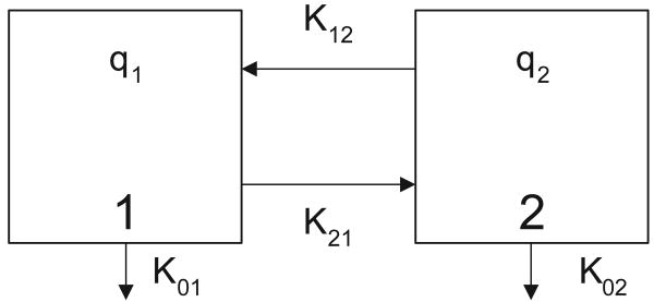
Let us consider the two-compartmental model depicted in Fig. 1. Assume that q_i(t) = v_ic_t, for i = 1, 2 denote the amount of a drug in a specific compartment. Here c_t is the concentration of a drug and v_t is the volume of the i-th compartment and K_ij is the fractional rate of transfer to compartment i from compartment j.

Figure 1. Two-compartment model system with the definition of model parameters.

A simple two-compartment model where the complete amount of drug from the first compartment enters into the second compartment can be written as [9]:

$$\begin{array}{lll}{\tau }^{{\alpha }_1-1}{{}_{0}D}_t^{\alpha 1}{q}_1(t)\hfill & =\hfill & -K_{21}{q}_1(t),\hfill \\ {\tau }^{{\alpha }_2-1}{{}_{0}D}_t^{\alpha 2}{q}_2(t)\hfill & =\hfill & K_{21}{q}_1(t)-K_{02}{q}_2(t),\hfill \end{array}$$ (11)

where we assumed K₀₁ = 0, K₁₂ = 0 and with the initial conditions q₁(0) = d₁ = dose, and q₂(0) = d₂ = 0.

The fractional compartment form of (11) is

$$\begin{array}{lll}{{}_{0}D}_t^{\alpha 1}{q}_1(t)\hfill & =\hfill & -k_{21}{q}_1(t),\hfill \\ {{}_{0}D}_t^{\alpha 2}{q}_2(t)\hfill & =\hfill & k_{21}{q}_1(t)-k_{02}{q}_2(t),\hfill \end{array}$$ (12)

with k₂₁ = K₂₁/τ^α1−1, k₂₁ = K₂₁/τ^α2−1, k₀₂ = K₀₂/τ^α2−1, τ^α1−1 = τ^α2−1, and for mass balance, α₁ = α₂.

The analytical solution of the model (12) has the following form [9]:

$$\begin{array}{lll}{q}_1(t)\hfill & =\hfill & d_1{E}_{{\alpha }_1,1}(-k_{21}{t}^{\alpha 1}),\hfill \\ q_2(t)\hfill & =\hfill & d_2{E}_{{\alpha }_2,1}(-k_{02}{t}^{\alpha 2})+d_1{\int }_0^t{(t-\tau )}^{{\alpha }_2-1}\times E_{{\alpha }_2,{\alpha }_2}[-k_{02}{(t-\tau )}^{{\alpha }_2}]E_{{\alpha }_1,1}(-k_{21}{\tau }^{{\alpha }_1})d\tau ,\hfill \end{array}$$ (13)

where we assume $q_1^{\prime }(0)=q_2^{\prime }(0)=0$ if α ∈ (0, 2].

The solution for q₁(t) and q₂(t) can be obtained for initial conditions d₁ and d₂, which correspond to the amounts of drug in the two compartments, with d₂ = 0. The concentration c₂ in the second compartment is given as c₂(t) = q₂(t)/v₂ and it has the form

$$\begin{array}{ccc}{c}_2(t)& =& d{\int }_0^t{(t-\tau )}^{{\alpha }_2-1}{E}_{{\alpha }_2,{\alpha }_2}[-k_{02}{(t-\tau )}^{{\alpha }_2}]\times E_{{\alpha }_1,1}(k_{21}{\tau }^{{\alpha }_1})d\tau \end{array}$$ (14)

where we consider the quotient d₁/v₂ = d as a parameter that depends on each subject separately. Note that d₁ (dose) is equal for all subjects and that α₁ = α₂ = α.

5 Numerical Solution and Simulations

The numerical solution of the fractional-order two-compartment model (12) is obtained by using relation (6) and it has the following form:

$$\begin{array}{lll}{q}_1(t_k)\hfill & =\hfill & (-k_{21}{q}_1(t_{k-1}))h^{{\alpha }_1}-\sum _{j=v}^k{c}_j^{({\alpha }_1)}{q}_1(t_{k-j}),\hfill \\ q_2(t_k)\hfill & =\hfill & (k_{21}{q}_1(t_k))-k_{02}{q}_2(t_{k-1})h^{{\alpha }_2}\sum _{j=v}^k{c}_j^{({\alpha }_2)}{q}_2(t_{k-j}),\hfill \end{array}$$ (15)

where T_sim is the simulation time, k = 1, 2, 3 …, N, for N = [T_sim/h], and (q₁(0), q₂(0)) is the start point (initial conditions). The binomial coefficients $c_j^{({\alpha }_i)}$, ∀i, are calculated according to relation (5) and v = 1, ∀k.

The experimental results from [9] show that for all subjects the drug concentration appeared in the blood only after some time, i.e., there was a time lag before the concentration started to rise. Also, for all subjects the drug concentration in the blood dropped to zero c₂(t) = 0, t > t* after some characteristic disappearance time t* ∈ [0, 24]. The study by [9] of 12 healthy female and male subjects followed the blood (plasma) level of diclofenac for 24 hours after a single dose oral administration of either the test formulation of (Hemofarm) tablets 100 (mg diclofenac/tab) or the reference formulation of (Geigy) tablets 100 (mg diclofenac/tab).

In [9] the kinetic parameters were determined through a least square numerical procedure applied to the measured data. The results are shown in Table 1. Here, subjects 1, 3, 6 and 9 were given the test formulation (Hemofarm), while subject 8 was given the reference formulation (Geigy).

Table 1. Parameters of the models.

Subject	α	k21 (h−α)	k02 (h−α)	d (mg/l)
1	0.93	2.89	2.74	30.17
3	0.90	1.58	2.65	42.68
6	0.60	0.90	1.68	35.00
8	1.00	0.34	0.37	4.00
9	0.68	1.37	1.27	21.98

In addition, for each subject, [9] plotted a comparison between the measured results and the fitted fractional-order model. In order to compare our model with the results of the [9] study, we first calculated the drug concentration using the Matlab function given in Appendix A and the relationship c₂(t) = q₂(t)/v₂. Note that d₁ (dose) is equal to 100 mg for all subjects.

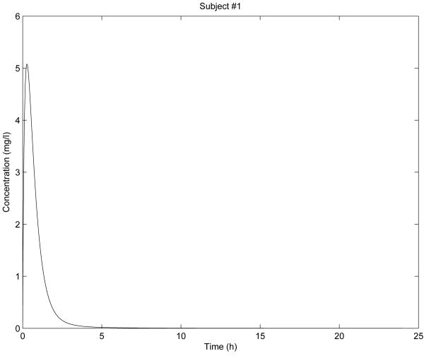
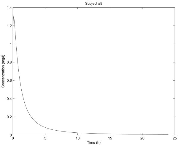
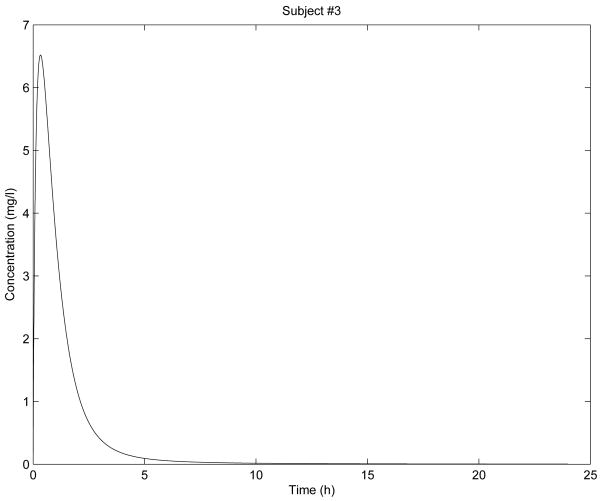
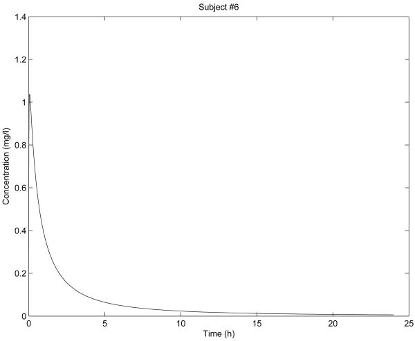
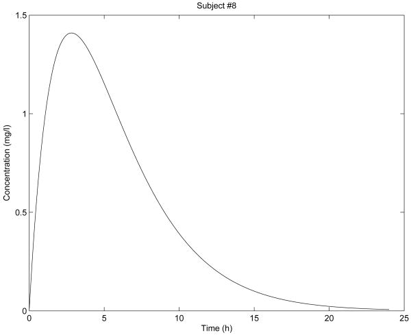
In Fig. 2 - Fig. 6 are shown the diclofenac concentration profiles from the test formulation and the reference formulation as a function of time for 5 subjects. From the results presented in Table 1 and Figures 2-6, we can see that the kinetics of the test formulation of diclofenac (Hemofarm) corresponds to a fractional order of less than one (0.93, 0.90, 0.60, and 0.68), while the reference formulation (Geigy) has an order of 1. These curves are very similar to those given by [9] where he found that while the kinetics of the test formulation of diclofenac depends both on the subject and the formulation. The peak blood concentrations in our curves are slightly different from those in the Popović study [9] because we estimated the parameter depending v₂, and hence the dose d in a different way d = d₁/v₂ for every subject.

Figure 2. Simulation for subject 1 parameters.

Figure 6. Simulation for subject 9 parameters.

Stability analysis of the fractional-order two-compartment model for each particular subject can be done by calculation of matrix (9) eigenvalues and by using a condition (10) for parameters given in Table 1. The stability analysis results can be summarized as follows:

As we can observe in Fig. 2 - Fig. 6, the results of stability analysis given in Table 2 confirm that solution of the fractional-order two-compartment model for each test subject is stable.

Table 2. Results of stability analysis.

Subject	α	eig(A)	|arg(eig(A))|	Result
1	0.93	−2.74, −2.89	π	stable
3	0.90	−2.65, −1.58	π	stable
6	0.60	−1.68, −0.90	π	stable
8	1.00	−0.34, −0.37	π	stable
9	0.68	−1.37, −1.27	π	stable

6 Discussion

The recent application of fractional calculus to multi-compartmental analysis [2, 9] is surprising in at least two ways. First, it is surprising that the fields of pharmacokinetics and pharmacodynamics, which are largely based upon systems of ordinary differential equations, have not been previously examined from the perspective of fractional calculus. Fractional calculus excels at simplifying the dynamics of complex, heterogeneous systems, and there is perhaps no more complicated system than one that tries to describe the uptake, distribution and elimination of drugs by animals and humans. Second, the application of fractional calculus to multi-compartmental drug distribution models is surprising to the degree that fundamental questions are just now arising about the dynamics of such processes [3, 10, 11].

In the field of fractional calculus, current workers are familiar with the difficulty in applied problems of pinning down the proper definition of the fractional derivative, its initial conditions, and its numerical evaluation for each situation. However, in multi-compartment pharmacokinetics, it is not these problems that confound, but the more basic question of how to configure the models in a correct and consistent manner so as to simplify the overall kinetic description without violating linearity, causality, consistency of units, and mass balance, as well as determining the physical meaning of fractional order rate constants. Fractional calculus has one of its strongest roots in modeling heat and mass transfer problems where diffusion is dominant. In pharmacokinetics the transfer of material - usually a drug - from one compartment to another (say, clearance from the blood to the urine in the kidney), is governed by selective filtration, glomerular permeability, bulk fluid flow and diffusion. Thus, we should anticipate success in this application, but not without - as the recent remarks [3, 10, 11] have presented - much discussion of the essential underlying assumptions of linearity, fractional order and mass conservation.

Nevertheless, even without a complete consensus on the proper models for multi-compartmental analysis, it is pleasing to see that all the key researchers are capturing useful information on drug kinetics by way of fractional order models of drug uptake and elimination kinetics [2, 9]. In the present study, we have added new Matlab tools to this analysis and shown that the simplest of cases (two-compartment model) can be solved in multiple ways (analytical, numerical, and via series expansions); all of which can provide essentially complete and useful information on drug kinetics and dynamics.

7 Conclusion

In this article we presented a numerical solution to a specific two-compartment fractional-order model with fractional derivatives of same order. The pharmacokinetics of diclofenac were consistent with the new model proposed by [9]. The numerical solution given in this article suggests possibilities for further investigations of the fractional-order model for various parameters and derivative orders. A Matlab function of the fractional kinetics for this model is presented in Appendix A, and it gives an interesting toolbox for the pharmaceutical scientist.

Figure 3. Simulation for subject 3 parameters.

Figure 4. Simulation for subject 6 parameters.

Figure 5. Simulation for subject 8 parameters.

A Matlab function

function [T,Y]=FO2CM(d1,k21,k02,d,orders,TSim)
%	Numerical solution of two compartments model
%
%	Input:	d1: dose
%		d: d1/v2
%		k21, k02: rate of compartment transfer
%		orders [alpha1,alpha2]: derivatives
%
%	Output:	T: simulation time (0 : Tstep : TSim)
%		Y: solution of model (q1=Y(1),q2=Y(2))
%
%	Authors:	(c) Ivo Petras (ivo.petras@tuke.sk)
%		(c) Richard L. Magin (rmagin@uic.edu)
%
%	Date: April, 2010.
%	time step of calculation:
h=0.0025;
%	number of calculated points:
n=round(t/h);
%	derivative orders:
alpha1=orders(1); alpha2=orders(2);
%	binomial coefficients:
cp1=1; cp2=1;
for	j=1:n
c1(j)=(1-(1+alpha1)/j)*cp1; cp1=c1(j);
c2(j)=(1-(1+alpha2)/j)*cp2; cp2=c2(j);
end
%	initial conditions:
q1(1)=d1; q2(1)=0.0;
%	calculation of the numerical solution:
for	i=2:n
q1(i)=(−k21*q1(i−1))*hˆalpha1 − memo(q1, c1, i);
q2(i)=(k21*q1(i)−k02*q2(i−1))*hˆalpha2 − memo(q2, c2, i);
end
for	j=1:n
	Y(j,1)=q1(j);
	Y(j,2)=q2(j);
end
T=0:h:TSim;
%
function [y] = memo(r, c, k)
%
temp = 0;
for	j=1:k-1
	temp = temp + c(j)*r(k−j);
end
y = temp;
%

References

- 1.Macheas P, Iliadis A. Modeling in Biopharmaceutics, Pharmacokinetics, and Phamacodynamics: Homogeneous and Heterogeneous Approaches. Springer Verlag; New York: 2006. [Google Scholar]
- 2.Dokoumetzidis A, Macheras P. Fractional kinetics in drug absorption and disposition processes. J Pharmacokinet Pharmacodyn. 2009;36:165–178. doi: 10.1007/s10928-009-9116-x. [DOI] [PubMed] [Google Scholar]
- 3.Dokoumetzidis A, Magin RL, Macheras P. A commentary on fractionalization of multi-compartmental models. J Pharmacokinet Pharmacodyn. 2010;37:203–207. doi: 10.1007/s10928-010-9153-5. [DOI] [PubMed] [Google Scholar]
- 4.Dorčák Ľ. Numerical Models for the Simulation of the Fractional-Order Control Systems, UEF-04-94, The Academy of Sciences, Inst of Experimental Physic. Košice, Slovakia: 1994. [Google Scholar]
- 5.Hilfer R. Applications of Fractional Calculus in Physics. Woeld Scientific Publishers; Singapore: 2000. [Google Scholar]
- 6.Magin RL. Fractional Calculus in Bioengineering. Begell House Publishers; 2006. [Google Scholar]
- 7.Matignon D. Stability properties for generalized fractional differential systems. Proc of Fractional Differential Systems: Models, Methods and App. 1998;5:145–158. [Google Scholar]
- 8.Podlubny I. Fractional Differential Equations. Academic Press; San Diego: 1999. [Google Scholar]
- 9.Popović JK, Atanacković MT, Pilipović AS, Rapaić MR, Pilipović S, Atanacković TM. A new approach to the compartmental analysis in pharmacokinetics: fractional time evolution of diclofenac. J Pharmacokinet Pharmacodyn. 2010;37:119–134. doi: 10.1007/s10928-009-9147-3. [DOI] [PubMed] [Google Scholar]
- 10.Popović JK, Atanacković MT, Pilipović AS, Rapaić MR, Pilipović S, Atanacković TM. Remarks on the mass balance for multi-compartmental models: a non-linear compartmental model. J Pharmacokinet Pharmacodyn. 2010;37:217–220. doi: 10.1007/s10928-009-9147-3. [DOI] [PubMed] [Google Scholar]
- 11.Verotta D. Fractional compartmental models and multi-term Mittag-Leffler functions. J Pharmacokinet Pharmacodyn. 2010;37:209–215. doi: 10.1007/s10928-010-9155-3. [DOI] [PMC free article] [PubMed] [Google Scholar]