Toward an Ising Model of Cancer and Beyond

Abstract

The holy grail of tumor modeling is to formulate theoretical and computational tools that can be utilized in the clinic to predict neoplastic progression and propose individualized optimal treatment strategies to control cancer growth. In order to develop such a predictive model, one must account for the numerous complex mechanisms involved in tumor growth. Here we review resarch work that we have done toward the development of an “Ising model” of cancer. The Ising model is an idealized statistical-mechanical model of ferromagnetism that is based on simple local-interaction rules, but nonetheless leads to basic insights and features of real magnets, such as phase transitions with a critical point. The review begins with a description of a minimalist four-dimensional (three dimensions in space and one in time) cellular automaton (CA) model of cancer in which healthy cells transition between states (proliferative, hypoxic, and necrotic) according to simple local rules and their present states, which can viewed as a stripped-down Ising model of cancer. This model is applied to model the growth of glioblastoma multiforme, the most malignant of brain cancers. This is followed by a discussion of the extension of the model to study the effect on the tumor dynamics and geometry of a mutated subpopulation. A discussion of how tumor growth is affected by chemotherapeutic treatment, including induced resistance, is then described. How angiogenesis as well as the heterogeneous and confined environment in which a tumor grows is incorporated in the CA model is discussed. The characterization of the level of organization of the invasive network around a solid tumor using spanning trees is subsequently described. Then, we describe open problems and future promising avenues for future research, including the need to develop better molecular-based models that incorporate the true heterogeneous environment over wide range of length and time scales (via imaging data), cell motility, oncogenes, tumor suppressor genes and cell-cell communication. A discussion about the need to bring to bear the powerful machinery of the theory of heterogeneous media to better understand the behavior of cancer in its microenvironment is presented. Finally, we propose the possibility of using optimization techniques, which have been used profitably to understand physical phenomena, in order to devise therapeutic (chemotherapy/radiation) strategies and to understand tumorigenesis itself.

1. Introduction

Cancer is not a single disease, but rather a highly complex and heterogeneous set of diseases. Dynamic changes in the genome, epigenome, transcriptome and proteome that result in the gain of function of oncoproteins or the loss of function of tumor suppressor proteins underlie the development of all cancers. While some of the mechanisms that govern the transformation of normal cells into malignant ones are rather well understood [1], many mechanisms are either not fully understood or are unknown at the moment. Even if all of the mechanisms could be identified and comprehended, it is not clear progress in understanding cancer could be made without knowledge of how these different mechanisms couple to one another. It has been observed that many complex interactions occur between tumor cells, and between a cancer and the host environment. Multidirectional feedback loops occur between tumor cells and the stroma, immune cells, extracellular matrix and vasculature [2, 3, 4, 5], which are not well understood synergistically. Clearly, our current state of knowledge is insufficient to deduce clinical outcome, not to mention how to control cancer progression in the most malignant forms of cancer.

This suggests that a more quantitative approach to understanding different cancers is necessary in order to control it and increase the lifetime of patients with these deadly diseases. Theoretical/computational modeling of cancer when appropriately linked with experiments and data offers a promising avenue for such an understanding. Such modeling of tumor growth using a variety of different approaches has been a very active area of research for the last two decades or so [6, 7, 8, 9, 10, 11, 12, 13, 14, 15, 16, 17, 18, 19, 20, 21, 22, 23, 24] but clearly is in its infancy. A diverse number of mechanisms have been explored via such models, and a multitude of computational/mathematical techniques have been employed; see Ref. [25] for a review. These models have the common aim of predicting certain features of tumor growth in the hope of finding new ways to control neoplastic progression. Given a model which yields reproducible and accurate predictions, the effects of different genetic, epigenetic and environmental changes, as well as the impact of therapeutically targeting different aspects of the tumor, can be probed. However, these models must be linked to data from experimental assays in a comprehensive and systematic fashion in order to develop of a quantitative understanding of cancer.

The holy grail of computational tumor modeling is to develop a simulation tool that can be utilized in the clinic to predict neoplastic progression and response to treatment. Not only must such a model incorporate the many feedback loops involved in neoplastic progression, the model must also account for the fact that cancer progression involves events occurring over a range of spatial and temporal scales [15]. A successful model would enable one to broaden the conclusions drawn from existing medical data, suggest new experiments, test new hypotheses, predict behavior in experimentally unobservable situations, and be employed for early detection.

There is overwhelming evidence that cancer of all types are emerging, opportunistic systems [26]. Success in treating various cancers as a self-organizing complex dynamical systems will require unconventional, innovative approaches and the combined effort of an interdisciplinary team of researchers. A lofty long-term goal of such an endeavor is not only to obtain a quantitative understanding of tumorigenesis but to limit and control the expansion of a solid tumor mass and the infiltration of cells from such masses into healthy tissue.

Because a comprehensive review of the vast literature concerning biophysical cancer modeling is beyond the scope of this article, we focus on reviewing the work that we have done toward the development of an “Ising model” of cancer. The Ising model is an idealized statistical-mechanical model of ferromagnetism that is based on simple local-interaction rules (see Figure 1), but nonetheless leads to basic insights and features of real magnets, such as phase transitions with a critical point. Toward the goal of developing an analogous Ising model of cancer, we have formulated a four-dimensional (4D) (three dimensions in space and one in time) cellular automaton (CA) model for brain tumor growth dynamics and its treatment [11, 12, 13, 18, 20, 21]. Like the Ising model for magnets, we will see later that this involves local rules for how healthy cells transition into various types of cancer cells. Before describing our computational models for tumor growth, we first briefly summarize several salient features of solid tumor growth as applied to glioblastoma multiforme (GBM), the most malignant of brain cancers.

Figure 1.

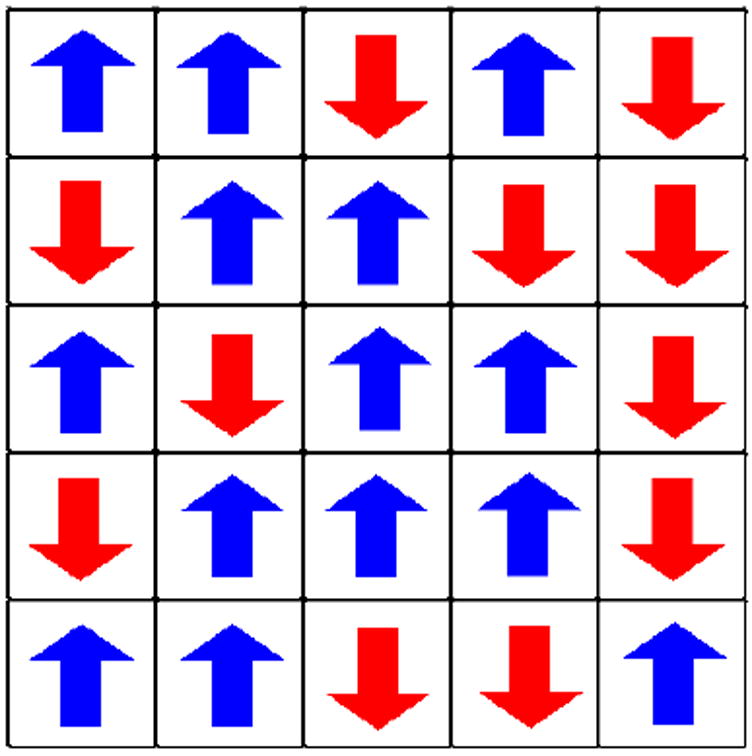
A schematic plot of the Ising model for an idealized ferromagnet. The model consists of spins that can be in one of two states (up or down) arranged in this case on a square lattice. In its simplest rendition, each spin interacts only with its nearest neighbors. Such simple local interaction rules can result in rich collective behavior depending on the temperature of the system.

The rest of paper is organized as follows: In Section 2, some background concerning GBMs and solid tumors in general is presented. In Section 3, a minimalist 4D CA tumor growth model is described in which healthy cells transition between states (proliferative, hypoxic, and necrotic) according to simple local rules and their present states, and apply it to GBMs. This is followed by a discussion of the extension of the model to study the effect on the tumor dynamics and geometry of a mutated subpopulation. How tumor growth is affected by chemotherapeutic treatment is also discussed, including induced resistance. In Section 4, the modification of the CA model to include explicitly the effects of vasculature evolution and angiogenesis on tumor growth are discussed. In Section 5, the effects of physical confinement and heterogeneous environment are described. In Section 6, a simulation tool for tumor growth that merges and improves individual CA models is presented. In Section 7, a descriptions if given of how one might characterize the invasive network organization around a solid tumor using spanning trees. Section 8 discusses some open problems and promising avenues for future research.

2. GBM and Solid Tumor Background

Glioblastoma multiforme (GBM) (see Figure 2), the most aggressive of the gliomas, is a collection of tumors arising from the glial cells or their precursors in the central nervous system [27]. Unfortunately, despite advances made in cancer biology, the median survival time for a patient diagnosed with GBM is only 12-15 months, a fact that has not changed significantly over the past several decades [28]. As suggested by its name (i.e., “multiforme”), GBM is complex at many levels of organization [27]. It exhibits diversity at the macroscopic level, having necrotic, hypoxic and proliferative regions. At the mesoscopic level, tumor cell interactions, microvascular remodeling [29] and pseudopalisading necrosis are observed [30]. Further, the discovery that tumor stem cells may be the sole malignant cell type with the ability to proliferate, self-renew and differentiate introduces yet another level of mesoscopic complexity to GBM [31, 32]. At the microscopic level, GBM cells exhibit point mutations, chromosomal deletions, and chromosomal amplifications [27].

Figure 2.

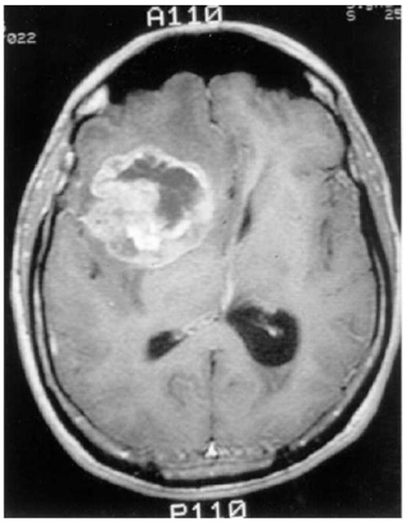
A T₁-contrast enhanced brain MRI-scan showing a right frontal GBM tumor, as adapted from Ref. [11]. Perifocal hypointensity is caused by significant edema formation. The hyper-intense, white region (ring-enhancement) reflects an area of extensive blood-brain/tumor barrier leakage. Since this regional neovascular setting provides tumor cells with sufficient nutrition it contains the highly metabolizing, e.g. dividing, tumor cells Therefore, this area corresponds to the outermost concentric shell of highly proliferating neoplastic cells in our model (see Figure 5).

A substantial amount of research has been conducted to model macroscopic tumor growth either based on microscopic considerations [33, 34, 35]; or in a more phenomenological fashion [6, 36]. One of the early attempts to model empircally the volume V of a solid tumor versus time t is the Gompertz model, i.e.,

$$V=V_0\exp (\frac{A}{B}[1-\exp (-\mathit{Bt})]),$$ (1)

where V₀ is the volume at time t = 0 and A and B are parameters; see Ref. [37] and references therein. Qualitatively, this equation gives exponential growth at small times which then saturates at large times (decelerating growth). In particular, this model considers the tumor as an oversized idealized multicellular tumor spheroid (see Figure 3), which is stage of early tumor growth. We note that modeling an ideal tumor as an oversized spheroid is especially suited for GBM, since this tumor, like a large MTS, comprises large areas of central necrosis surrounded by a rapidly expanding shell of viable cells (Figure 2). However, we note that real tumors always possess much more complex morphology. More importantly, Gompertzian-growth models are very limited; they only capture gross features of tumor growth and cannot explain their underlying “microscopic” mechanisms.

Figure 3.

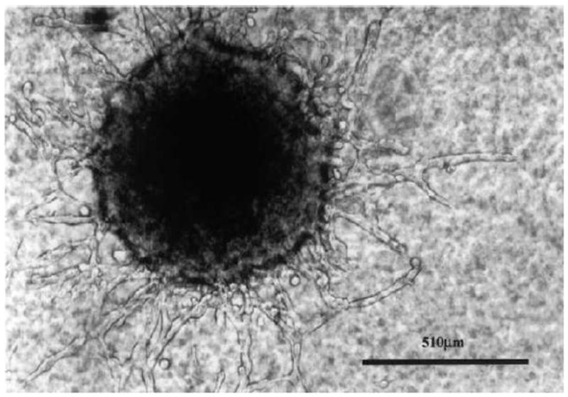
MTS-gel assay showing a central spheroid with multiple “chain”-like invasion pathways leading towards the boundary (magnification: x 200), as adapted from Ref. [11].

One of the hallmarks of high-grade malignant neuroepithelial tumors, such as glioblastoma multiforme (GBM), is the regional heterogeneity, i.e., the relatively large number of clonal strains or subpopulations present within an individual tumor of monoclonal origin [38, 39, 40]. Each of these strains is characterized by specific properties, such as the rate of division or the level of susceptibility to treatment [41]. Therefore the growth dynamics of a single tumor are determined by the relative behaviors of each separate subpopulation. For example, the appearance of a rapidly dividing strain can substantially bias tumor growth in that direction. Tumors supposedly harbor cells with an increased mutation rate, which indicates that these tumors are genetically unstable [42, 43, 44]. Genetic and epigenetic events throughout the tumor may occur randomly or be triggered by environmental and intrinsic stresses. The continuing existence of a subpopulation, however, depends primarily on the subpopulation’s ability to compete with the dominant population in its immediate vicinity.

Clonal heterogeneity within a tumor has been shown to have very pronounced effects on treatment efficacy [45, 46]. Treatment resistance is itself a complex phenomenon. There is no single cause of resistance, and many biochemical aspects of resistance are poorly understood. Chemoresistant strains can either be resistant to a single drug or drug family (individual resistance), or they can be resistant to an array of agents (multidrug/pleotropic resistance) [47]. Cellular mechanisms behind multidrug resistance include increased chemical efflux and/or decreased chemical influx, such as with P-glycoprotein-mediated (P-gp) drug resistance [48, 49].

Complicating the situation further, resistance can arise at variable times during tumor development. Some tumors are resistant to chemotherapy from the onset. This has been described as inherent resistance, because it exists before chemotherapeutic drugs are ever introduced. In other cases, however, treatment initially proves successful, and only later does the tumor prove resistant. This is an example of acquired resistance, as it develops in response to treatment [47]. There are at least two possible mechanisms for this type of tumor behavior. Acquired resistance may result from a small number of resistant cells that are gradually selected for throughout the course of treatment. At the same time, there is also evidence suggesting that chemotherapeutic agents may induce genetic or epigenetic changes within tumor cells, leading to a resistant phenotype [50]. Other studies indicate that chemotherapy may increase cellular levels of P-gp mRNA and protein in various forms of human cancer [51, 52]. A tumor’s response to radiation therapy can also depend on underlying genetic factors. A cell’s inherent radio-resistance may stem from the efficiency of DNA repair mechanisms in sublethally damaged cells [53, 54, 55].

While the properties of GBM cells are very important in understanding growth dynamics, just as important are the properties of the environment in which the tumor grows. For example, GBMs grow in either the brain or spinal cord, and are therefore confined by the shape and size of these organs [20]. Another example of the importance of accounting for the host environment relates to the vascular structure of the brain.

Recent research evidence suggests that tumors arising in vascularized tissue such as the brain do not originate avascularly [29], as originally thought. Instead, it is hypothesized that glioma growth is a process involving vessel co-option, regression and growth. Three key proteins, vascular endothelial growth factor (VEGF) and the angiopoietins, angiopoietin-1 (Ang-1) and angiopoietin-2 (Ang-2), are required to mediate these processes [29]. A picture of what likely occurs during the process of glioma vascularization has been summarized by Gevertz and Torquato [18]. As a malignant mass grows, the tumor cells co-opt the mature vessels of the surrounding brain that express constant levels of bound Ang-1. Vessel co-option leads to the upregulation in Ang-2 and this shifts the ratio of bound Ang-2 to bound Ang-1. In the absence of VEGF, this shift destabilizes the co-opted vessels within the tumor center and marks them for regression [56, 57]. Vessel regression in the absence of vessel growth leads to the formation of hypoxic regions in the tumor mass. Hypoxia induces the expression of VEGF, stimulating the growth of new blood vessels [58]. This robust angiogenic response eventually rescues the suffocating tumor. Glioma growth dynamics remain intricately tied to the continuing processes of vessel regression and growth.

Tumor cell invasion is a hallmark of gliomas [59]. Individual glioma cells have been observed to spread diffusely over long distances and can migrate into regions of the brain essential for the survival of the patient [27]. While MRI scans can recognize mass tumor lesions, these scans are not sensitive enough to identify malignant cells that have spread well beyond the tumor region [60]. Typically, when a solid tumor is removed, these invasive cells are left behind and tumor recurrence is almost inevitable [27].

Numerous models have been developed to model certain tumor behavior or characteristics with a great deal of mathematical rigor (e.g., in the form of coupled differential equations). However, with such approaches, the sets of equations that govern tumor behavior often do not correspond to the characteristics of individual tumor cells. An important goal of studying tumor development is to illustrate how their macroscopic traits stem from their microscopic properties. In addition, most of the equations are problem-specific, which limits their utility as general tools for tumor study. Another potential challenge is that tumor models should be appreciated by as diverse an audience as possible. Ideally, the mathematical complexity that allows theoreticians to analyze subtle aspects of it should not be an obstacle for clinicians who treat GBM. A model that accounts for complex tumor behavior with relative mathematical ease could be valuable.

To this end, we have developed what appears to be a powerful cellular automaton (CA) computational tool for tumor modeling. Based on a few salient set of microscopic parameters, this CA model can realistically model the macroscopic tumor behavior, including growth dynamics, emergence of a subpopulation as well as the effects of tumor treatment and resistance [11, 12, 13]. This model has been extended to study the effects of vasculature evolution on early tumor growth and to simulate tumor growth in confined heterogeneous environments [18, 20, 21]. We have also developed mathematical models to characterize the invasive network organization around a solid tumor [61].

3. Toward an Ising Model of Cancer Growth

In this section, we describe a four-dimensional (4D) cellular automaton (CA) model that we have developed that describes tumor growth as a function of time, using the fewest number of microscopic parameters [11, 12, 13]. We refer to this as a minimalist four-dimensional (4D) model because it involves three spatial dimensions and one dimension in time with the goal of capturing the salient features of tumor growth with a minimal number of parameters. The algorithm takes into account that this growth starts out from a few cells, passes through a multicellular tumor spheroid (MTS) stage (Figure 3) and proceeds to the macroscopic stages at clinically designated time-points for a virtual patient: detectable lesion, diagnosis and death. This 4D CA algorithm models macroscopic GBM tumors as an enormous idealized MTS, mathematically described by a Gompertz-function given by Eq. (1), since this tumor, like a large MTS, comprises large areas of central necrosis surrounded by a rapidly expanding shell of viable cells (Figure 2). In accordance with experimental data, the algorithm also implicitly takes into account that invasive cells are continually shed from the tumor surface and implicitly assumes that the tumor mass is well-vascularized during the entire process of growth. The effects of vasculature evolution are considered explicitly in Sections 5 and 7.

3.1. A 4D Cellular Automaton Model

A CA model is a spatially and temporally discrete model that consists of a grid of cells, with each cell being in one of a number of predefined states. The state of a cell at a given point in time depends on the state of itself and its neighbors at the previous discrete time point. Transitions between states are determined by a set of local rules. The simulation is designed to predict clinically important criteria such as the fraction of the tumor which is able to divide (GF), the non-proliferative (G₀/G₁ arrest) and necrotic fractions, as well as the rate of growth (volumetric doubling time) at given radii. Furthermore, this CA model enables one to study emergence of a subpopulation due to cell mutations as well as the effects of tumor treatment and resistance. The general CA model includes both a proliferation routine which models tumor growth by cell division and a treatment routine which models the cell response to treatment and cell mutations. It also incorporates a novel adaptive automaton cell generation procedure. In particular, the CA model is characterized by several biologically important features:

• The model is able to grow the tumor from a very small size of roughly 1000 real cells through to a fully developed tumor with 10¹¹ cells. This allows a tumor to be grown from almost any starting point, through to maturity.

• The thickness of different tumor layers, i.e. the proliferative rim and the non-proliferative shell, are linked to the overall tumor radius by a 2/3 power relation. This reflects a surface area to volume ratio, which can be biologically interpreted as nutrients diffusing through a surface.

• The discrete nature of the model and the variable density lattice allow us to control the inclusion of mutant “hot spots” in the tumor as well as variable cell sensitivity/resistance to treatment. The variable density lattice will allow us to look at such an area at a higher resolution.

• Our inclusion of mechanical confinement pressure enables us to simulate the physiological confinement by the skull at different locations within the brain differently.

Our CA algorithm can be broken into three parts: automaton cell generation, the proliferation routine and the treatment routine. In the ensuing discussions, we first present the three parts of our algorithm. Then we show that the our model reflects a test case derived from the medical literature very well, proving the hypothesis that macroscopic tumor growth behavior may be modeled with primarily microscopic data.

3.1.1. Cellular Automaton Cell Generation

The first step of the simulation is to generate the automaton cells. The underlying lattice for the algorithm is the Delaunay triangulation, which is the dual lattice of the Voronoi tessellation [11, 62]. In order to develop the automaton cells, a prescribed number of random points are generated in the unit square using the process of random sequential addition (RSA) of hard circular disks. In the RSA procedure, as a random point is generated, it is checked if the point falls within some prescribed distance from any other point already placed in the system [11, 62]. Points that fall too close to any other point are rejected, and all others are added to the system. Each cell in the final Voronoi lattice will contain exactly one of these accepted sites. The Voronoi cell is defined by the region of space nearer to a particular site than any other site. In two-dimensions, this results in a collection of polygons that fill the plane.

Because a real brain tumor grows over several orders of magnitude in volume, the lattice was designed to allowed continuous variation with the radius of the tumor. The density of lattice sites near the center was significantly higher than that at the edge. A higher site density corresponds to less real cells per automaton cell, and so to a higher resolution. The higher density at the center enables us to simulate the flat small-time behavior of the Gompertz curve. In the current model, the innermost automaton cells represent roughly 100 real cells, while the outermost automaton cells represent roughly 10⁶ real cells. The average distance between lattice sites was described by the following relation:

$$\zeta =\frac{1}{6}{r}^{2/3}$$ (2)

in which ζ is the average distance between lattice sites and r is the radial position at which the density is being measured. This relation restricts the increase in the number of proliferating cells as the tumor grows. Note that when modeling the effects of vasculature evolution discussed in the following, a a uniform lattice is used for which each automaton cell includes approximately 10 real cancer cells.

3.1.2. Minimalist 4D Proliferation Algorithm

The proliferation algorithm is designed to allow a tumor consisting of a few automaton cells, representing roughly 1000 real cells, to grow to a full macroscopic size. An idealized model of a macroscopic tumor is an almost spherical body consisting of concentric shells of necrotic, non-proliferative and proliferative regions (see Figure 5). The four microscopic growth parameters of the algorithm are p₀, a, b, and R_max reflecting, respectively, the rate at which the proliferative cells divide, the nutritional needs of the non-proliferative and proliferative cells, and the response of the tumor to mechanical pressure within the skull. In addition, there are four key time-dependent quantities that determine the dynamics of the tumor, i.e., R_t, δ_p, δ_n, p_d giving, respectively, the average overall tumor radius, proliferative rim thickness, non-proliferative thickness and probability of division. These quantities are based on the four parameters (p₀, a, b, R_max) and are calculated according to the following algorithm.

Figure 5.

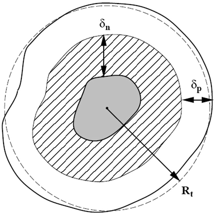
A cross-section of an idealized solid tumor, as adapted from Ref. [11]. The inner gray region is composed of necrotic tissue. The cross-hatched layer is composed of living, quiescent cells (non-proliferative). It has a thickness δ_n. The outer shell, with thickness δ_p, is composed of proliferative cells. Both length scales δ_n and δ_p are determined by nutritional needs of the cells via diffusional transport.

• Initial setup: The cells within a fixed initial radius of the center of the grid are designated proliferative. All other cells are designated as non-tumorous.

• Time is discretized and incremented, so that at each time step:

  • Each cell is checked for type: non-tumorous or (apoptotic and) necrotic, non-proliferative or proliferative tumorous cells.

  • Non-tumorous cells and tumorous necrotic cells are inert.

  • Non-proliferative (growth-arrested) cells more than a certain distance, δ_n, from the tumor’s edge are turned necrotic. This is designed to model the effects of a nutritional gradient. The edge of the tumor is taken to be the nearest non-tumorous cell, i.e.,

    $${\delta }_n=a{R}_t^{2/3}.$$ (3)
  • Proliferative cells are checked to see if they will attempt to divide according to the probability of division, p_d, which is influenced by the location of the dividing cell, reflecting the effects of mechanical confinement pressure. This effect requires the use of an additional parameter, the maximum tumor extent, R_max. p_d is given by

    $$p_d=p_0(1-\frac{r}{R_{\mathit{max}}})$$ (4)
  • If a cell attempts to divide, it will search for sufficient space for the new cell beginning with its nearest neighbors and expanding outwards until either an empty (non-tumorous) space is found or nothing is found within the proliferation radius, δ_p. The radius searched is calculated as:

    $${\delta }_p=b{R}_t^{2/3}.$$ (5)

  • If a cell attempts to divide but cannot find space it is turned into a non-proliferative cell.

• After a predetermined amount of time has been stepped through, the volume and radius of the tumor are plotted as a function of time.

• The type of cell contained in each grid are saved at given times.

The above simulation procedure is also illustrated in Figure 6. We note that the redefinition of the proliferative to non-proliferative transition implemented in the algorithm is one of the most important new features of the model. They allow a larger number of cells to divide, since cells no longer need to be on the outermost surface of the tumor to divide. In addition, it ensured that cells that cannot divide are correctly labeled as such. Table 1 summarizes the important time-dependent functions calculated by the proliferation algorithm and the constant growth parameters used. The readers are referred to Ref. [11] for the detailed description of the algorithm and parameters.

Figure 6.

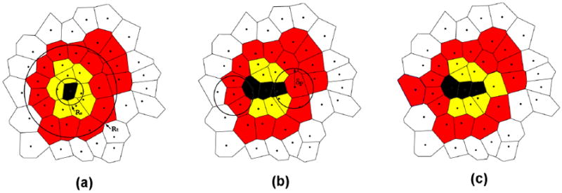
An illustration of the minimalist proliferation algorithm through a cross-section of the solid tumor [11]. (a) A tumor contains necrotic (black), non-proliferative (yellow or light gray) and proliferative cells (red or dark gray). The average overall tumor radius R_t and the necrotic region radius R_n are shown. (b) Two non-proliferative cells that more than δ_n away from the tumor edge are turned into necrotic and two proliferative cells are selected with probability p_d to check for division. If there are non-tumorous cells within a distance δ_d from the selected proliferative cell, it will divide; otherwise, it will turn into a non-proliferative cell. (c) One of the selected proliferative cell divides and the other turns into a non-proliferative cell.

Table 1.

The time-dependent functions and growth, treatment parameters for the model.

Functions within the model (time dependent)
Rt	Average overall tumor radius (see Appendix)
δp	Proliferative rim thickness (determines growth fraction)
δn	Non-proliferative thickness (determines necrotic fraction)
pd	Probability of division (varies with time and position)
Growth parameters
p0	Base probability of division, linked to cell-doubling time (0.192)
a	Base necrotic thickness, controlled by nutritional needs (0.42 mm1/3)
b	Base proliferative thickness, controlled by nutritional needs (0.11 mm1/3)
Rmax	Maximum tumor extent, controlled by pressure response (38 mm)

3.1.3. Extending the 4D CA Model to Study Emergence of a Subpopulation

Malignant brain tumors such as GBM generally consist of a number of distinct subclonal populations. Each of these subpopulations, arising from the constant genetic and epigenetic alteration of existing cells in the rapidly growing tumor, may be characterized by its own behaviors and properties. However, since each single cell mutation only leads to a small number of offspring initially, very few newly arisen subpopulations survive more than a short time. Kansal et al [12] have extended the CA to quantify “emergence,” i.e. the likelihood of an isolated subpopulation surviving for an extended period of time. Only mutations affecting the rate of cellular division were considered in this rendition of the model. In addition, only competition between clones was taken into account; there were no cooperative effects included, although such effects can easily be incorporated.

The simulation procedure is as follows: an initial tumor composed entirely of cells of the primary clonal population is introduced, which is allowed to grow using the proliferation algorithm until it reaches a predetermined average overall radius. Then, a single (or a small number of) automaton cell is changed from the primary strain to a secondary strain with an altered probability of division, which represents very small fractions of the total population of proliferative tumor cells and the tumor is allowed to continue to grow using the proliferation algorithm. It is important to note that this does not represent a single mutation event but rather a mutation event that results in a subpopulation reaching a size dictated by the limits of the lattice resolution employed (i.e., a specified number of cells).

The behavior of the secondary strain was characterized in terms of two properties: the degree α and the relative size β of the initial population of mutated cells, i.e.,

$$\alpha =\frac{p_1}{p_0},$$ (6)

which represents the ratio between the base probability of division of the new clone, p₁, and that of the original clone, p₀; and

$$\beta =\frac{\mathrm{volume\; of\; proliferating\; cells\; of\; the\; new\; clone}}{\mathrm{volume\; of\; proliferating\; cells\; of\; the\; original\; clone}}.$$ (7)

Positive, negative and no competitive advantages are respectively conferred for α > 1, α < 1, and α = 1. The initial value β, i.e., β₀ = β(t = 0), is a parameter of the model reflecting the size of the mutated region introduced.

3.1.4. Extending the 4D CA Model to Study Treatment

Besides the four growth parameters in the minimalist 4D CA model, three additional parameters for treatment were subsequently introduced: γ, ∊, and ϕ, the values of which reflect, respectively, the proliferative cells’ treatment sensitivity, the non-proliferative cells’ treatment sensitivity, and the mutational response of the tumor cells to treatment [13]. Furthermore, there are three additional time-dependent quantities D_pro, D_non and β, giving respectively fraction of proliferative cells that die upon treatment (equivalent to γ), fraction of non-proliferative cells that die upon treatment (equivalent to γ∊) and volume fraction of mutated living cells. These parameters are summarized in Table 2 and a detailed discussion is given in Ref. [13].

Table 2.

Treatment parameters and associated terms for the model.

Treatment parameters
γ	Governs the proliferative cells’ response at each instance of treatment (0.55 – 0.95)
∊	Allows for different treatment responses between proliferative and non-proliferative cells (0 – 0.4)
ϕ	Fraction of surviving proliferative cells that mutate in response to treatment (10−5 – 10−2)
Other Terms
Dpro	Fraction of proliferative cells that die upon treatment; equivalent to γ
Dnon	Fraction of non-proliferative cells that die upon treatment; equivalent to γ∊
β	Volumetric fraction of living cells (proliferative and non-proliferative) belonging to the secondary strain

In the simulation, treatment was introduced as “periodic impulse”, i.e., a small tumor mass is introduced which is intended to represent a GBM after successful surgical resection and allowed to grow using the proliferation algorithm; then treatment is applied and considered effective at discrete time points. In particular, the simulation proceeds through the proliferative steps until every n_w week time-point, at which time the treatment routine is introduced:

• After the last round of cellular division, each proliferative cell is checked to see if it is killed by the treatment. The probability of death for a given proliferative cell D_pro is given by

  $$D_{\mathit{pro}}=\gamma ,$$ (8)

  where γ ∈ (0, 1) is the proliferative treatment parameter. Dead proliferative automaton cells are converted to healthy cells.
• Each non-proliferative cell is checked to see if it is killed. The probability of death for a given non-proliferative cell D_non is given by

  $$D_{\mathit{non}}=\gamma \epsilon ,$$ (9)

  where ∊ ∈ (0, 1) is the non-proliferative treatment parameter and D_non is a fraction of D_pro. A non-proliferative cell is converted to a necrotic cell upon death.

• Each surviving non-proliferative cell is checked to see if it is within the proliferative thickness of a healthy cell (i.e. the tumor surface). If so, the non-proliferative cell is converted back to a proliferative cell.

• All proliferative cells (including newly-designated ones) are checked for mutations for treatment resistance γ with probability ϕ. A new γ ∈ (0, 1) is randomly generated for mutated cells while ∊ remains constant.

Clinically, GBM treatment consists of both radiation therapy and chemotherapy. However, in our model we do not distinguish between the separate effects of these two methods. The tumors’ response to all treatment is captured by the treatment algorithm. Moreover, this response is assumed to be instantaneous at each four-week time point.

4. Putting the 4D CA Model Through Its Paces

4.1. A Test Case for Proliferation Algorithm

The tumor growth data generated via the minimalist 4D CA proliferation algorithm was compared with available experimental data for an untreated GBM tumor from the medical literature [11]. The parameters compared were cell number, growth fraction, necrotic fraction and volumetric doubling time, which are used to determine a tumor’s level of malignancy and the prognosis for its future growth. Because it is impossible to determine the exact time a tumor began growing, the medical data are listed at fixed radii. The different cell fractions used were extrapolated from the spheroid level and compared to data published for cell fractions at macroscopic stages.

Summarized in Table 3 is the comparison between simulation results and data (experimental, as well as clinical) taken from the medical literature (see Ref. [11] for detailed references). The simulation data were created using a tumor which was grown from an initial radius of 0.1 mm. The following parameter set (see Table 1) was used:

$$p_0=0.192,a=0.42{\mathrm{mm}}^{1/3},b=0.11{\mathrm{mm}}^{1/3},R_{\mathit{max}}=37.5\mathrm{mm}$$

This value of p₀ corresponds to a cell-doubling time of 4.0 days. The parameters a and b have been chosen to give a growth history that quantitatively fits the test case. The specification of these parameters corresponds to the specification of a clonal strain. The parameter R_max was similarly chosen to match the test case history. In this case, however, the fit is relatively insensitive to the value of R_max, as long as the parameter is somewhat larger than the fatal radius in the test case. On the whole, the simulation data reproduces the test case very well. The virtual patient would die roughly 11 months after the tumor radius reached 5 mm and 3.5 months after the expected time of diagnosis. The fatal tumor volume is about 65 cm³.

Table 3.

Comparison of simulated tumor growth and experimental data. For each quantity, the simulation data is give on the first line and the experimental data is given on the second line.

	Spheroid	Det. Les.	Diagnosis	Death
Time	Day 69	Day 223	Day 454	Day 560
Radius	0.5 mm	5 mm	18.5 mm	25 mm
	0.5 mm	5 mm	18.5 mm	25 mm
Cell No.	106	109	5 × 1010	1011
	7 × 105	6 × 108	4 × 1010	9 × 1010
Growth fraction	0.36	0.30	0.20	0.09
	0.35	0.30	0.18	0.11
Necrotic fraction	0.46	0.49	0.55	0.60
	0.38	0.53	0.58	0.63
Volume-doubling time	6 days	45 days	70 days	105 days
	9 days	36 days	68 days	100 days

Central cross-sections of the tumors are shown in Figure 7, in which the growth of the tumor can be followed graphically over time. Here necrotic cells are labeled with black, non-proliferative tumorous cells with light gray and proliferative tumor cells with dark gray. A cut-away view of the simulated tumor is shown in Figure 8. As expected in this idealized case, the tumor is essentially spherical, within a small degree of randomness. The high degree of spherical symmetry ensures that the central cross-section is a representative view. The volume and radius of the developing tumor are shown versus time in Figure 9. Note that the virtual patient dies while the untreated tumor is in the rapid growth phase.

Figure 7.

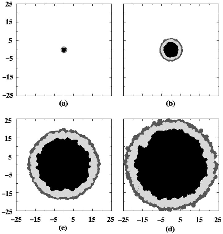
The development of the central section of a tumor as a function of time, as adapted from Ref. [11]. Correspond to: (a) the initial tumor spheroid stage, (b) time to first detectable lesion, (c) time at diagnosis and (d) time at death. The dark gray outer region is comprised of proliferating cells, the light gray is non-proliferative cells and the black is necrotic cells. The length scales are given in millimeters.

Figure 8.

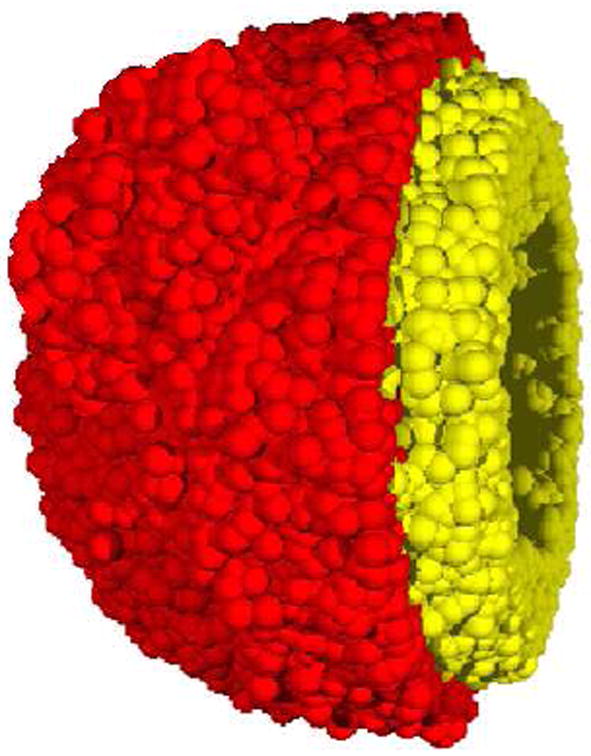
A cut-away view a simulated tumor generated from the minimalist CA algorithm [11]. The inner necrotic core is not depicted in this view. The yellow (light gray) region is comprised of nonproliferative cells and the red (dark gray) shell depicts the proliferative cells.

Figure 9.

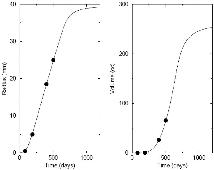
Plots of the radius and volume of the tumor versus time, as adapted from Ref. [11]. The lines correspond to simulation predictions, using the first parameter set given in the text. The plotted points reflect the test case derived from the medical literature. A quantitative comparison of the simulation with the test case is given in Table 2.

4.2. Modeling the Emergence of A Subpopulation

Recall that the parameter α reflects the degree of advantage of the mutated subpopulation over the primary clone (positive, negative and no competitive advantages are respectively conferred for α > 1, α < 1, and α = 1) and the initial value β, i.e., β₀ = β(t = 0), is a parameter of the model reflecting the size of the mutated region introduced. A subpopulation is considered to have emerged once it comprises 5% of the actively dividing cell population or if it remains in the actively dividing state once the tumor has reached a fully developed size. Numerous simulations (at least 100) were run at each parameter set by Kansal et al [12] in order to calculate the expected probabilities of emergence, i.e.,

$$P=\frac{\mathrm{number\; of\; trials\; in\; which\; emergence\; occurs}}{\mathrm{total\; number\; of\; trials}}.$$ (10)

along with confidence intervals, σ, defined as

$$\sigma =\sqrt{\frac{\overline{p}(1-\overline{p})}{N}}$$ (11)

where p̄ represents the observed probability of emergence in N trials. We note that the probability of emergence is actually a conditional probability: it is the probability that a subpopulation with a mutation of degree α emerges given that a region of relative size β₀ has mutated.

The results represented were run with a parameter set in which

$$\begin{array}{c}{p}_0=0.192,p_1={\mathit{\alpha p}}_0,a=0.42{\mathrm{mm}}^{1/3},\\ b=0.11{\mathrm{mm}}^{1/3},R_{\mathit{max}}=37.5\mathrm{mm}\end{array}$$

for the primary strain, in a simulation in which each time step represents one day [12]. Figure 10 depicts the observed probability of emergence, P, for a subpopulation of initial size β₀ = 6 × 10⁻⁵ as a function of α, which gives an approximation of the true, asymptotic, probability of emergence. Also shown in Figure 10 is a cut-away view of the simulated tumor with a subpopulation. Not surprisingly, P is a monotonically increasing function that tends to 0 for α < 1 and to 1 as α become significantly greater than 1.

Figure 10.

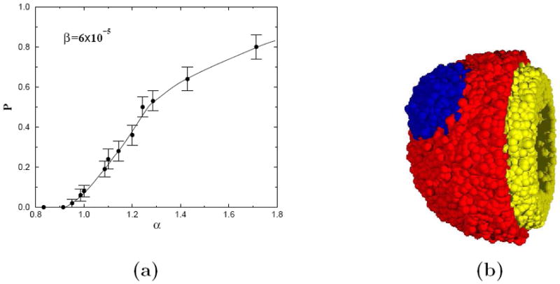
(a) A plot of probability of emergence P versus the degree of mutation α, i.e., growth advantage (α > 1) or disadvantage (α < 1), as adapted from Ref. [12]. The error bars indicate confidence intervals defined by one standard deviation from the mean. Each data point represents the average of roughly 100 simulated tumors. The line is drawn as a guide for the eye. (b) A cut-away view a simulated tumor with a mutated population. The inner necrotic core is not depicted in this view. The yellow (light gray) region is comprised of nonproliferative cells and the red (dark gray) shell depicts the proliferative cells of the primary strain and the blue (darker gray) shows the proliferative cells of the secondary strain.

Perhaps the most striking feature of these results is that there is a non-zero probability of emergence for a very small population with no growth rate advantage, or even with a small disadvantage (i.e. α ≈ 0.95). This suggests that a mutated subpopulation may arise even without any growth advantage. These populations could represent “dormant” clones which confer an advantage not being selected for at the time. An example would be the appearance of hypoxia tolerant or even treatment resistant clones. It should be stressed that populations with less competitive advantages over other tumor strains can have a nonzero probability of emergence especially if they are localized in space, which leads to a minimum surface area between the two populations per unit tumor volume. In this way, the population with smaller competitive advantage can compete more effectively. We will see in the next subsection that this same principle is at work when resistance is induced due to treatment. It was also found that the emergence probability P is a monotonically increasing function in β₀ and has a logarithmic dependence on β₀ [12].

Figure 11 shows the effects of growth of the subpopulation on the tumor geometry. It can be seen clearly that the center of mass of the tumor is significantly shifted by the emergence of the subpopulation. Another example of the importance of subpopulations is depicted in Figure 12 [12]. In this example, a diagnosis was made (on day t₀) giving information about the macroscopic size and growth rate of the tumor. From this information three possible growth histories of the tumor are plotted. One is the time history of the tumor with an emergent subpopulation. The others represent limiting cases, each with a monoclonal tumor of either the primary (“base p₀”) or secondary (“high p₀”) clonal strain. Note that at the time of diagnosis all three scenarios have very similar dynamics. So any of the three histories is a reasonable prediction given only size and growth rate information. However, estimating a fatal tumor volume to be 65 cm³ and defining the survival time to be the time required to reach this volume, the base case mis-predicts survival times to be 90 days, which is 30 days more than the 60 days of the “true” course.

Figure 11.

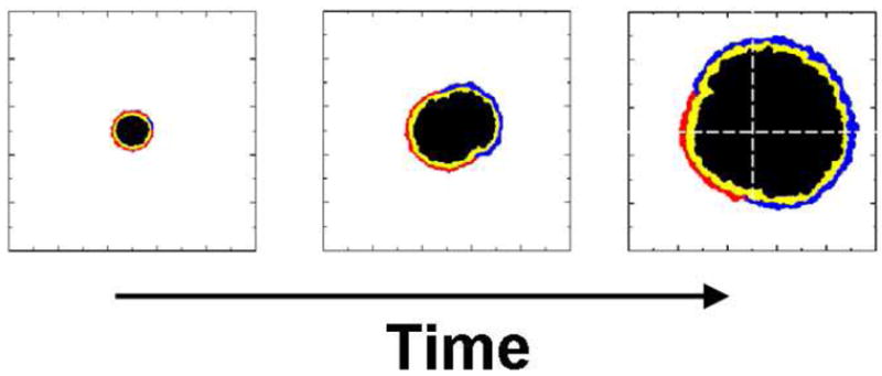
The effects of the emergence of a subpopulation on the tumor geometry, as adapted from Ref. [12]. The center of mass of the tumor is significantly shifted as the growth of the subpopulation,

Figure 12.

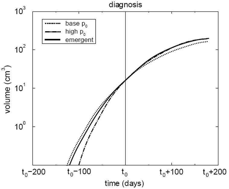
Volume of a simulated tumor with an emergent subpopulation in time, as adapted from Ref. [12]. Volumes of tumors composed entirely of the primary strain and the secondary strain are also shown and labeled “base p₀” and “high p₀,” respectively. Each tumor is set to have the same volume at some “diagnosis” time t₀. Note that the emerging tumor’s dynamics initially follow the base case, but later follow the highly aggressive case.

It is noteworthy that from this perspective the overall future growth dynamics of the entire tumor closely follows that of the most aggressive case, indicating that the more aggressive clone dominates overall outcome and should therefore also define the appropriate treatment. This finding supports the current practice in pathology of grading tumors according to the most malignant area (i.e. population) found in any biopsy material. Although of less clinical significance, the high case similarly mis-predicts the past history of the tumor. If the diagnosis had been made earlier, the base case would yield still worse future predictions. Similarly the “high” p₀ case would yield worse past predictions for a diagnosis made at a later time. The predictive errors arising from the assumption of a monoclonal tumor indicate how important an accurate estimate of the clonal composition of a tumor is in establishing a complete history and prognosis. Note that the numbers given here are intended to show the scale of the inaccuracy possible, not to reflect any data extracted from actual patients.

4.3. Modeling the Effects of Tumor Treatment and Resistance

Combining the proliferation algorithm and the treatment algorithm, the behavior of tumors that are able to develop resistance throughout the course of treatment were investigated [13]. Recall that additional parameters were introduced in the treatment routine: γ, ∊, and ϕ, the values of which reflect, respectively, the proliferative cells’ treatment sensitivity, the non-proliferative cells’ treatment sensitivity, and the mutational response of the tumor cells to treatment (see Table 2).

These investigation consisted of three individual case studies. In Case 1, the growth dynamics of monoclonal tumors are studied to determine how tumor behavior is affected by the treatment parameters γ and ∊. Case 2 builds upon this information, analyzing the behavior of two-strain tumors. Here, a secondary treatment-resistant strain exists alongside a primary treatment-sensitive strain. A secondary sub-population was introduced at the onset of each simulation, initializing it in different spatial arrangements and at several (small) relative volumes. In both Cases 1 and 2, no additional sub-populations arise in the tumors once the simulation has begun (i.e. ϕ = 0). In Case 3, however, tumors were studied that were capable of undergoing resistance mutations in response to each round of treatment (ϕ > 0). In these simulations, the growth and morphology of the tumors were analyzed in relation to the fraction of mutating cells.

Here we only report on the results of Cases 2 and 3. In Case 2, the smaller subpopulation of a secondary treatment-resistant strain was initially spatially distributed in two different ways on the tumor surface that primarily consist of the primary treatment-sensitive strain: a localized and scattered scenario, reflecting possible effects of the result of surgery, for example (see Figure 13). In the simulation, the tumors were initialized as a single strain, i.e., monoclonally with γ = 0.95 and ∊ = 0.05 and treatment was introduced every four weeks while the tumor is growing from a small mass with a radius of 4mm, corresponding to approximately 99% of surgical volume resection. For the scattered resistance scenario, the resistant strain was found to compete more effectively with the sensitive strain and it was shown that the initial number of resistant cells were not a significant indicator or prognosis.

Figure 13.

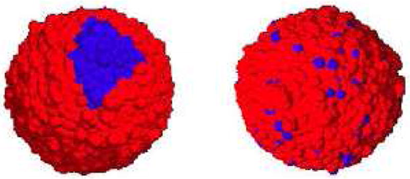
Initial images of two-strain tumors, as adapted from Ref. [13]. The resistant subpolulation is localized (left panel) and scattered (right panel). The blue cells of each tumor belong to the resistant subpopulation, while the blues ones belong to the sensitive subpopoluation.

These conclusions may at first glance seem to contradict the those reported by by Kansal et al [12]. Recall that in this work the selection pressure was different (growth-rate competition versus treatment effects). Moreover, the roles of the primary and secondary strains are reversed in the Case 2 example: the primary strain possessed a competitive advantage over the secondary strain. Nevertheless, the conclusions of both papers [12, 13] follow precisely the same principle. The proliferative ability of a strain with a competitive advantage varies directly with its contact area with the less comptetive strain per cell.

Unlike Case 2, the tumors in Case 3 begin the simulations as a single strain. Here, however, treatment can induce the appearance of mutant strains (ϕ > 0). In these simulations, the growth and morphology of the tumors were analyzed in relation to the fraction of mutating cells. The tumors in Case 3 are all initialized monoclonally with γ = 0.95 and ∊ = 0.05. With this initial γ-value, nearly every mutant strain that arises from the initial population will posses a lower γ-value. This is not to suggest that all induced mutations must possess increased resistance. This fact here merely stems from the initial sensitive tumor under consideration.

At first, the tumors in Case 3 will develop like treatment-sensitive, monoclonal tumors; growth will then accelerate as resistant cells begin to dominate. This corresponds to a case of acquired resistance via induced (genetic and epigenetic) mutations. Overall, the tumor dynamics here are more variable than in Cases 1 and 2. When a new strain appears, it begins as a single automaton cell. Unlike Case 2, not all new strains will be able to proliferate to an appreciable extent. Some are overwhelmed by the parent strain from which they arise.

The mean survival time of the tumors were determined as a function of ϕ and these data are summarized in Figure 14. plots this data; From ϕ = 10⁻⁵ to ϕ = 10⁻², the survival times vary nearly logarithmically with ϕ. When ϕ = 10⁻⁵, the mean time is near 27 months, as most tumors remain monoclonal (or nearly monoclonal) with γ = 0.95, ∊ = 0.05. As ϕ increases, resistant strains appear more commonly and survival times fall.

Figure 14.

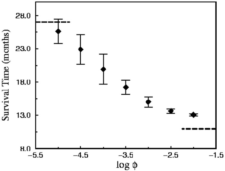
Survival times associated with continuously mutating tumors, as adapted from Ref. [13]. This figure depicts data of the mean survival time (with error bars) as a function of ϕ, the expected fraction of tumor cells that mutate at each instance of treatment.

One of the more intriguing observations in this case involves the gross morphology of the mutating tumors. Their three-dimensional geometries exhibit an interesting dependence on the value of ϕ. Figure 15 presents representative images of the fully-developed tumors for small, intermediate and large fractions of mutated proliferative cells ϕ after treatment. For small ϕ (left panel of Figure 15), some tumors develop a secondary strain while others do not. The tumors that remain monoclonal maintain their spherical geometry. When a resistant sub-population does develop, it appears as a lobe on the parental tumor. For intermediate ϕ, resistant sub-populations consistently arise from the parental strain. The middle panel of Figure 15 depicts a typical tumor, whose geometries consistently deviate from an ideal sphere. These tumors are multi-lobed in appearance, and the original strain is commonly overwhelmed. However, when ϕ is large, the geometric trend reverses, i.e., the tumors (right panel of Figure 15) again appear more spherical, despite the fact that they experience the greatest fraction of mutations per treatment event. These images suggest that extreme mutational responses can lead to similar macroscopic geometries. Non-spherical geometries result from intermediate ϕ-values.

Figure 15.

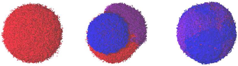
Images of continuously mutating tumors, as adapted from Ref. [13]. Shown are representative images of tumors with small ϕ (left panel), intermediate ϕ (middle panel) and large ϕ (right panel). The distinct clonal sub-populations in each tumor are represented with a different color, ranging from red (highest γ-values) to violet (lowest γ-values). All tumors here are fully-developed.

5. Modeling the Effects of Vasculature Evolution

As pointed out in the Introduction, there are complex interactions occurring between between a tumor and the host environment, which makes it very difficult in predicting clinical outcome, even if mutations responsible for oncogenesis that determine tumor growth are beginning to be understood. These interactions include the effects of vasculature evolution on tumor growth, the organ-imposed physical confinement as well as the host heterogeneity. While the three studies described in the previous section were successful at analyzing and characterizing GBM growth both with and without treatment, in each case, the CA model made the simplifying assumption that the tumor mass was well-vascularized (the vascular network and angiogenesis were implicitly accounted for) and the effects of mechanical confinement were limited to one parameter (R_max), which allowed for growth of spherically symmetric tumors with a maximum radius. Spherical-like growth is realistic provided that the environment is effectively homogeneous, but heterogeneous environments will cause apsherically-shaped tumors.

In order to incorporate a greater level of microscopic detail, a 3D (two dimensions in space and one in time) hybrid variant of the original CA model that allows one to study how changes in the tumor vasculature due to vessel co-option, regression and sprouting influence GBM was developed by Gevertz and Torquato [18]. This computational algorithm is based on the co-option-regression-growth experimental model of tumor vasculature evolution [29, 56]. In this model, as a malignant mass grows, the tumor cells co-opt the mature vessels of the surrounding tissue that express constant levels of bound angiopoietin-1 (Ang-1). Vessel co-option leads to the upregulation of the antagonist of Ang-1, angiopoietin-2 (Ang-2). In the absence of the anti-apoptotic signal triggered by vascular endothelial growth factor (VEGF), this shift destabilizes the co-opted vessels within the tumor center and marks them for regression [29, 56]. Vessel regression in the absence of vessel growth leads to the formation of hypoxic regions in the tumor mass. Hypoxia induces the expression of VEGF, stimulating the growth of new blood vessels.

A system of reaction-diffusion equations was developed to track the spatial and temporal evolution of the aforementioned key factors involved in blood vessel growth and regression [18] (see Section 6 for a detailed description). Based on a set of algorithmic rules, the concentration of each protein and bound receptor at a blood vessel determines if a vessel will divide, regress or remain stagnant. The structure of the blood vessel network, in turn, is used to estimate the oxygen concentration at each cell site. Oxygen levels determine the proliferative capacity of each automaton cell. The reader is referred to [18] for the full details of this algorithm. The model proved to quantitatively agree with experimental observations on the growth of tumors when angiogenesis is successfully initiated and when angiogenesis is inhibited. Further, due to the biological details incorporated into the model, the algorithm was used to explore tumor response to a variety of single and multimodal treatment strategies [18].

6. Modeling the Effects of Physical Confinement and Heterogeneous Environment

An assumption made in both the original CA algorithm and the one that explicitly incorporates vascular evolution is that the tumor is growing in a spherically symmetric fashion. In a study performed by Helmlinger et al [63], it was shown that neoplastic growth is spherically symmetric only when the environment in which the tumor is developing imposes no physical boundaries on growth. In particular, it was demonstrated that human adenocarcinoma cells grown in a 0.7% gel that is placed in a cylindrical glass tube develop to take on an ellipsoidal shape, driven by the geometry of the capillary tube. However, when the same cells are grown in the same gel outside the capillary tube, a spherical mass develops [63]. This experiment clearly highlights that the assumption of radially symmetric growth is only valid when a tumor grows in an unconfined or spherically symmetric environment.

Since many organs, including the brain and spinal cord, impose non-radially symmetric physical confinement on tumor growth, the original CA algorithm was modified to incorporate boundary and heterogeneity effects on neoplastic progression [20]. The first modification that was made to the original algorithm was simply to specify and account for the boundary that is confining tumor growth. Several modifications were made to the original automaton rules to account for the impact of this boundary on neoplastic progression. The original CA algorithm imposed radial symmetry in order to determine whether a cancer cell is proliferative, hypoxic, or necrotic. The assumption of radially symmetric growth was also utilized in determining the probability a proliferative cell divides. In order to allow tumor growth in any confining environment, all assumptions of radial symmetry from the automaton evolution rules were removed. It was demonstrated that models that do not account for the geometry of the confining boundary and the heterogeneity in tissue structure lead to inaccurate predictions on tumor size, shape and spread (the distribution of cells throughout the growth-permitting region). The readers are referred to Ref. [20] for the details of this investigation, but an illustration of confinement effects are given in the next section.

7. A Merged Tool for Growing Heterogeneous Tumors In Silico

7.1. Algorithmic Details

Each of the previously discussed algorithms were designed to answer a particular set of questions and successfully served their purpose. Hence, Gevertz and Torquato [21] merged each algorithm into a single cancer simulation tool that would not only accomplish what each individual algorithm had accomplished, but had the capacity to have emergent properties not identifiable prior to model integration. In developing the merged algorithm, some modifications were made to the original automaton rules to more realistically mimic tumor progression. The merged simulation tool is summarized as follows:

1. Automaton cell generation: A Voronoi tessellation of random points generated using the nonequilibrium procedure of random sequential addition of hard disks determines the underlying lattice for our algorithm [11, 62]. Here a uniform density lattice is used instead of the lattice with variable density. Each automaton cell created via this procedure represents a cluster of a very small number of biological cells (~ 10).

2. Define confining boundary: Each automaton cell is divided into one of two regimes: nonmalignant cells within the confining boundary and nonmalignant cells outside of the boundary.

3. Healthy microvascular network: The blood vessel network which supplies the cells in the tissue region of interest with oxygen and nutrients is generated using the random analog of the Krogh cylinder model detailed in Ref. [18]. One aspect of the merger involved limiting blood vessel development to the subset of space in which tumor growth occurs.

4. Initialize tumor: Designate a chosen nonmalignant cell inside the growth-permitting environment as a proliferative cancer cell.

5. Tumor growth algorithm: Time is then discretized into units that represent one real day. At each time step:

   1. Solve PDEs: A previously-developed system of partial differential equations [18] is numerically solved one day forward in time. The quantities that govern vasculature evolution, and hence are included in the equations, are concentrations of VEGF (v), unoccupied VEGFR-2 receptors (r_v0), the VEGFR-2 receptor occupied with VEGF (r_v), Ang-1 (a₁), Ang-2 (a₂), the unoccupied angiopoietin receptor Tie-2 (r_a0), the Tie-2 receptor occupied with Ang-1 (r_a1) and the Tie-2 receptor occupied with Ang-2 (r_a2). The parameters in these equations include diffusion coefficients of protein x (D_x), production rates b_x and b̄_x, carrying capacities K_x, association and dissociation rates (k_y and k_−y) and decay rates μ_x. Any term with a subscript i denotes an indicator function; for example, p_i is a proliferative cell indicator function. It equals 1 if a proliferative cell is present in a particular region of space, and it equals 0 otherwise. Likewise, h_i is the hypoxic cell indicator function, n_i is necrotic cell indicator function and e_i is the endothelial cell indicator function. The equations solved at each step of the algorithm are:

      $$\frac{\mathit{\partial }v}{\mathit{\partial }t}=D_v\mathrm{\Delta }v+b_v{h}_i(h-v^2/K_v)-k_0{\mathit{vr}}_{v0}+k_{-0}{r}_v-{\mu }_{v}v$$ (12)

      $$\frac{\mathit{\partial }{a}_1}{\mathit{\partial }t}=b_{a1}{e}_i(p_i+h_i+n_i)(e_0-a_1^2/K_a)-k_1{a}_1{r}_{a0}+k_{-1}{r}_{a1}-{\mu }_{a1}{a}_1$$ (13)

      $$\begin{array}{ll}\frac{\mathit{\partial }{a}_2}{\mathit{\partial }t}& =D_{a2}\mathrm{\Delta }{a}_2+b_{a2}{e}_i(p_i+h_i+n_i)(e_0-a_2^2/K_a)\\ & +{\overline{b}}_{a2}{h}_i(h-a_2^2/K_a)-k_2{a}_2{r}_{a0}+k_{-2}{r}_{a2}-{\mu }_{a2}{a}_2\end{array}$$ (14)

      $$\frac{\mathit{\partial }{r}_{v0}}{\mathit{\partial }t}=-k_{0}v{r}_{v0}+k_{-0}{r}_v$$ (15)

      $$\frac{\mathit{\partial }{r}_{a0}}{\mathit{\partial }t}=-k_1{a}_1{r}_{a0}+k_{-1}{r}_{a1}-k_2{a}_2{r}_{a0}+k_{-2}{r}_{a2}$$ (16)

      $$\frac{\mathit{\partial }{r}_v}{\mathit{\partial }t}=k_0{\mathit{vr}}_{v0}-k_{-0}{r}_v$$ (17)

      $$\frac{\mathit{\partial }{r}_{a1}}{\mathit{\partial }t}=k_1{a}_1{r}_{a0}-k_{-1}{r}_{a1}$$ (18)

      $$\frac{\mathit{\partial }{r}_{a2}}{\mathit{\partial }t}=k_2{a}_2{r}_{a0}-k_{-2}{r}_{a2}$$ (19)

      In these equations, h(x, y, t) represents the concentration of hypoxic cells and e₀ represents the endothelial cell concentration per blood vessel. The system of differential equations contains 21 parameters, 13 of which were taken from experimental data. Parameters were unable to be found in the literature were estimated. For more details on the parameter values, as well as information on the initial and boundary conditions and the numerical solver, the reader is referred to Ref [18].
   2. Vessel Evolution: Check whether each vessel meets the requirements for regression or growth. Vessels with a concentration of bound Ang-2 six times greater than that of bound Ang-1 regress [57], provided that the concentration of bound VEGF is below its critical value. Vessel tips with a sufficient amount of bound VEGF sprout along the VEGF gradient.
   3. Nonmalignant Cells: Healthy cells undergo apoptosis if vessel regression causes its oxygen concentration to drop below a critical threshold (more particularly, if the distance of a healthy cell from a blood vessel exceeds the assumed diffusion length of oxygen, 250 μm). Further, nonmalignant cells do not divide in the model. While nonmalignant cell division occurs in some organs, a hallmark of neoplastic growth is that tumor cells replicate significantly faster than the corresponding normal cells. Hence, we work under the simplifying assumption that nonmalignant division rates are so small compared to neoplastic division rates that they become relatively unimportant in the time scales being considered. In the cases where this assumption does not hold, nonmalignant cellular division would have to be incorporated into the model.
   4. Inert Cells: Tumorous necrotic cells are inert. This assumption is certainly valid for the tumor type that motivated this modeling work, glioblastoma multiforme. In the case of glioblastoma, the presence of necrosis is an important diagnostic feature and, in fact, negatively correlates with patient prognosis.
   5. Hypoxic Cells: A hypoxic cell turns proliferative if its oxygen level exceeds a specified threshold [18] and turns necrotic if the cell has survived under sustained hypoxia for a specified number of days. In the original algorithms, the transition from hypoxia to necrosis was based on an oxygen concentration threshold. However, given that cells (both tumorous and nonmalignant alike) have been shown to have a limited lifespan under sustained hypoxic conditions, a temporal switch more accurately describes the hypoxic to necrotic transition. Thus, a novel aspect of the merged algorithm is a temporal hypoxic to necrotic transition. It has been measured that human tumor cells remain viable in hypoxic regions of a variety of xenografts for 4-10 days [18]. In our simulations, we will use the upper-end of this measurement and assume that tumor cells can survive under sustained hypoxia for 10 days.
   6. Proliferative Cells: A proliferative cell turns hypoxic if its oxygen level drops below a specified threshold. However, if the oxygen level is sufficiently high, the cell attempts to divide into the space of a viable nonmalignant cell in the growth-permitting region. The probability of division p_div is given by

      $$p_{\mathit{div}}=p_0(1-r/L_{\mathit{max}})$$ (20)

      where p₀ is the base probability of division, r is the distance of the dividing cell from the geometric center of the tumor and L_max is the distance between the closest boundary cell in the direction of tumor growth and the tumor’s center. In the original implementations of the algorithm, p₀ was fixed to be 0.192, giving a cell-doubling time of ln(2)/ln(1 + p₀) ≈ 4 days. In the merged algorithm proposed here, we wanted to account for fact that tumor cells with a higher oxygen concentration likely have a larger probability of dividing than those with a lower oxygen concentration. For this reason, we have modified the algorithm so that p₀ depends on the distance to the closest blood vessel d_vessel (which is proportional to the oxygen concentration at a given cell site). The average value of p₀ was fixed to be 0.192, and we have specified that p₀ takes on a minimum value p_min of 0.1 and a maximum value p_max of 0.284. This means that a proliferative cell in the model can have a cell doubling time anywhere in the range of three to seven days. The formula used to determine p₀ is

      $$p_0=\frac{p_{\mathit{min}}-p_{\mathit{max}}}{D_{o2}}{d}_{\mathit{vessel}}+p_{\mathit{max}},$$ (21)

      where D_O2 is the diffusion length of oxygen, taken to be 250 μm [20, 18]. Both p_min and p_max depend on the average probability of division. If this average probability changes, so does p_min and p_max.
   7. Tumor Center and Area: After each cell has evolved, recalculate the geometric center and area of the tumor.

The readers are referred to Ref. [21] for more details, including how cell-level phenotypic heterogeneity is also considered in a similar fashion to the manner done in Refs [12] and [13].

7.2. Simulating Heterogeneous Tumor Growth

The 3D cancer simulation tool described here was employed to study tumor growth in a confined environment: a two-dimensional representation of the cranium in space as a function of time [21]. The cranium is idealized as an elliptical growth-permitting environment with two growth-prohibiting circular obstacles representing the ventricular cavities. Tumor growth is initiated in between a ventricular cavity and the cranium wall. In this setting, we find that the early-time characteristics of the tumor and the vasculature are not significantly different than those observed when radial symmetry is imposed on tumor growth. In particular, after 45 days of growth (Figure 16(a)), vessels associated with the radially symmetric tumor begin to regress and hypoxia results in the tumor center. Twenty days later (Figure 16(b)), a strong, disordered angiogenic response has occurred in the still radially symmetric tumor. Over the next 50 days of growth (Figure 16(c) and (d)), the disorganized angiogenic blood vessel network continues to vascularized the growing tumor, but the tumor’s shape begins to deviate from that of a circle due to the presence of the confining boundary. The patterns of vascularization observed are consistent with the patterns observed in the original vascular model [18], suggesting that the merged algorithm maintains the functionality of the original vascular algorithm.

Figure 16.

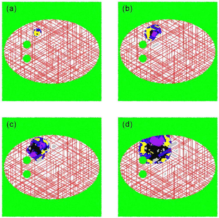
The temporal development of a tumor growing in a two-dimensional representation of the cranium in space, as adapted from Ref. [21]. (a) After 40 days, the dimensionless area is 0.0049 units², with 30% of the cells being proliferative, 66.4% being hypoxic and 3.6% being necrotic. (b) After 65 days, the dimensionless area is 0.0195 units², with 51.2% of the cells being proliferative, 33.0% being hypoxic and 15.8% being necrotic. (c) After 85 days, the dimensionless area is 0.0362 units², with 48.2% of the cells being proliferative, 16.8% being hypoxic and 35.0% being necrotic. (d) After 115 days, the dimensionless area is 0.0716 units², with 45.1% of the cells being proliferative, 18.6% being hypoxic and 36.3% being necrotic. The deep blue outer region (darkest of the grays in black and white) is comprised of proliferative cells, the yellow region (lightest of the grays in black and white) consists of hypoxic cells and the black center contains necrotic cells. Green cells (intermediate gray shade in black and white) are apoptotic. The white speckled region of space represents locations in which the tumor cannot grow. The lines represent blood vessels. If viewing the image in color, red vessels were part of the original tissue vasculature, and the purple vessels grew via angiogenesis.

However, if the results of this simulation are compared with those of the environmentally-constrained algorithm without the explicit incorporation of the vasculature [20], we find that the merged model responds to the environmental constraints in a way that is more physically intuitive. In the original environmentally-constrained algorithm [20], the tumor responds quickly and drastically to the confining boundary and ventricular cavities. This occurs because the original evolution rules not only determine the probability of division based on the distance to the boundary, but also determine the state of a cell based on a measure of its distance to the boundary. In the merged model which explicitly incorporates the vasculature, the state of each cell depends on the blood vessel network, and only the probability of division directly depends on the boundary. For this reason, the merged algorithm exhibits an emergent property in that it grows tumors that respond more gradually and naturally to environmental constraints than does the algorithm without the vasculature.

The tumor growth in a two-dimensional irregular region of space that truly allows the neoplasm to adapt its shape as it grows in time (i.e., a 3D model) was also investigated by Gevertz et al [20]; see also Gevertz and Torquato [21]. As with the two-dimensional representation of the cranium in space, an emergent property of the merged algorithm in which that a more subtle and natural response to the effects of physical confinement is found occurs. The studies taking into account mutations responsible for phenotypic heterogeneity have been carried out by Gevertz and Torquato [21], to which the readers are referred for more details. We note that all the results presented in this section need to be validated experimentally.

8. Analysis of the Invasion Network: Minimal Spanning Trees

It is well known that cancer cells can break off the main tumor mass and invade healthy tissue. For many cancers, this process can eventually result in metastases to other organs. Tumor-cell invasion is a hallmark of glioblastomas, as individual tumor cells have been observed to spread diffusely over long distances and can migrate into regions of the brain essential for the survival of the patient [27]. In certain cases, the invading tumor cells form branched chains (see Figure 3), i.e., tree structures [61]. The brain offers these invading cells a variety of pathways they can invade along (such as blood vessel and white fiber tracts), which may be interpreted as the edges of an underlying graph with the various “resistances” values along these pathways playing the role of edge weights. The underlying physics behind the formation of the observed patterns are only beginning to be understood.

The competition between local and global driving forces is a crucial factor is determining the structural organization in a wide variety of naturally occurring branched networks [64, 65, 66]. As an attempt toward a model of the invasive network emanating from a solid tumor, Kansal and Torquato [61] investigated the impact of a global minimization criterion versus a local one on the structure of spanning trees. Spanning trees are defined as a loopless, connected set of edges that connect all of the nodes in the underlying graph (see Figure 17). In particular, these authors considered the generalized minimal spanning tree (GMST) and generalized invasive spanning tree (GIST), because they generally offer extremes of global (GMST) and local (GIST) criteria. Both GMST and GIST are defined on graphs in which the nodes are partitioned into groups and each edge has an assigned weight. GMST is refined (relative to that of a spanning tree) such that the requirement that every node of the graph is included in the tree is replaced by the inclusion of at least one node from each group with the additional requirement that the total weight of tree is minimized [67]. GIST can be constructed by growing a connected cluster of edges by “invading” the remaining the edge with the minimal weight at its boundary with the requirement of the inclusion of at least one node from each group in the final tree [61].

Figure 17.

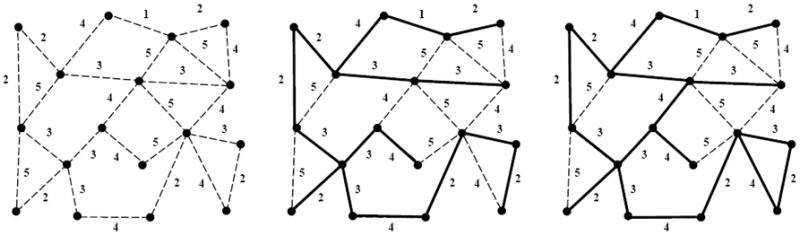
Example of a weighted graph and the resulting minimal spanning tree, as adapted from Ref. [61]. (a) Shows all of the edges and nodes in a graph, with the weight of each edge indicated next to the edge. Graph edges are depicted by broken lines. (b) Shows the minimal spanning tree for this graph, which is the set of edges that connects every node in the graph in the tree with the lowest total weight. Edges included in the tree are shown as solid lines, while edges not included remain broken lines. The total weight of the tree in (b) is 40, and the occupied edge density (number of edges included in the tree divided by total number of edges in the graph) is 15/25 = 0.6. (c) Shows the invasion percolation network for the same graph. Note that the invasion percolation network may have loops and in this case there are two closed loops. If loop formation is prevented (resulting in the highest weight edge in any loop remaining unoccupied) the result is the acyclic invasion percolation network. As can be readily seen by comparing figures (b) and (c) the acyclic invasion percolation network is identical to the minimal spanning tree.

Kansal and Torquato [61] have developed efficient algorithms to generate both GMST and GIST structures, as well as a method to convert GIST structure incrementally into a more globally optimized GMST-like structure (see Figure 18). The readers are referred to the original paper for more algorithmic details. These methods allow various structural features to be observed as a function of the degree to which either criterion is imposed and the intermediate structures can then serve as benchmarks for comparison when a real image is analyzed.

Figure 18.

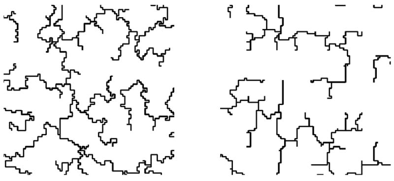
Examples of (a) backbone of generalized invasive spanning tree (GIST) (b) generalized minimal spanning tree (GMST), as adapted from Ref. [61].

We note that a general procedure by which information extracted from a single, fixed network structure can be utilized to understand the physical processes which guided the formation of that structure is highly desirable in understanding the invasion network of tumor cells, since the temporal development of such a network is extremely difficult to observe. To this end, Kansal and Torquato [61] examined a variety of structural characterizations and found that the occupied edge density (i.e., the fraction of edges in the graph that are included in the tree) and the tortuosity of the arcs in the trees (i.e., the average of the ratio of the path length between two arbitrary nodes in the tree and the Euclidean distance between them) correlate well with the degree to which an intermediate structure resembles the GMST or GIST. Since both characterizations are straightforward to determine from an image (e.g., only the information of the tree is required for tortuosity and additional information of underlying graph is needed for occupied edge density), they are potentially useful tools in the analysis of the formation of invasion network structures. Once the distribution of the invasive cells in the brain is understood, a cellular automaton simulation tool for glioblastoma that is useful in a clinical setting could be developed. This of course would apply more generally to invasion networks around other solid tumors.

9. Conclusions and Future Work

In this paper, we have reviewed the work that we have performed to attempt to develop an Ising model of cancer. We began by describing a minimalist 4D cellular automaton model of cancer in which healthy cells transition between states (proliferative, hypoxic, and necrotic) according to simple local rules and their present states, which can viewed as a stripped-down Ising model of cancer [11, 12, 13]. Using four proliferation parameters, this model was shown to reflect the growth dynamics of a clinically untreated tumor very well [11]. This was followed by discussion of an extension of the model to study the effect on the tumor dynamics and geometry of a mutated subpopulation [12] and how tumor growth is affected by chemotherapeutic treatment, including induced resistance, with additional three treatment parameters [13]. An improved CA model that explicitly accounts for angiogenesis [18] as well as the heterogeneous and confined environment in which a tumor grows [20] were discussed. A general cancer simulation tool that merges, adapts and improves all of the aforementioned mechanism into a single CA model was also presented and applied to simulate the growth the GBM in a vascularized confined cranium [21]. Finally, we touched on how one might characterize the invasive network organization (local versus global organization) around a solid tumor using spanning trees [61]. However, we must move well beyond the improved CA model as well as other computational models of cancer in order to make real progress on controlling this dreaded set of diseases.

9.1. The Obvious but Necessary

Formulating theoretical and computational tools that can be utilized clinically to predict neoplastic progression and propose individualized optimal treatment strategies to control cancer growth is the holy grail of tumor modeling. Although the development of our most comprehensive cellular automaton model is potentially a useful step towards the long-term goal of an Ising model for cancer, numerous complex mechanisms involved in tumor growth and their interactions needs to be identified and understood in order to truly achieve this goal.

For example, an effective Ising model of cancer must incorporate molecular-level information via a better understanding of the cellular origin of the tumor. Such information might become available if imaging techniques for spatial statistics of cell/molecular heterogeneity can be developed. This would enable an improved understanding of invading cancer cells: cell motility, cell-cell communication and phenotypes of invading cells. Such knowledge is crucial in order to predict the effects of treatment and tumor recurrence. The incorporation of stem cells, oncogenes and tumor suppressor genes in computational models would aid in our understanding of tumor progression.

In addition, we must quantitatively characterize the biological (host) environment (i.e., a heterogeneous material/medium) in which cancer evolves, including both the microstructure and the associated physical properties. For example, a better knowledge of diffusion and transport of nutrients, drugs, etc. would significantly improve the accuracy of the model simulating the effects of vasculature evolution and treatment. Similarly, cell mechanics and mechanical stresses must be understood. In such cases, imaging of the biological environment over a wide spectrum of length and time scales will be crucial.

It is important to emphasize that the theory heterogeneous media is a huge field within the physical sciences that can be brought to bear to better understand the host heterogeneous microenvironment of cancer and metastases (see Figure 19). For example, there exist powerful and sophisticated theoretical/computational techniques to characterize the microstructure of heterogeneous materials and predict their physical properties [62]. Specifically, the details of complex microstructures are described in terms of various statistical descriptors (different types of correlation functions), which in turn determine the physical properties of the heterogeneous materials [62]. In particular, the effective properties that have been predicted include the diffusion coefficient [68], reaction rates [69, 70], elastic/viscoelastic moduli [71, 72], thermal conductivity [73], thermal expansion coefficient [74], fluid permeability [75], and electrical conductivity [76, 77]. Accurate characterizations of these properties of the host environment and tumor mass are essential in order to significantly improve models for tumor growth and invasion. For example, a knowledge of the elastic properties enables one to better model the effects of physical confinement and the mechanical response of solid tumor; while the diffusion coefficient and fluid permeability are crucial to model transport of nutrients and proteins, delivery of drugs and even the migration of cancer cells. These techniques have been used to propose a novel biologically constrained three-phase model of the brain microstructure [78].

Figure 19.

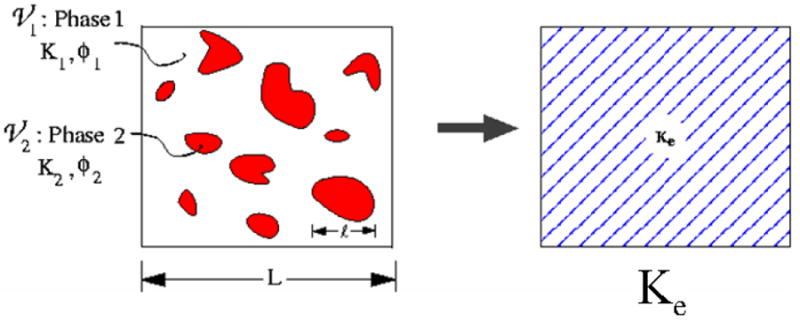
A schematic illustration of heterogeneous materials, as adapted from Ref. [62]. Left panel: A two-phase heterogeneous material with properties K₁ and K₂ and volume fractions ϕ₁ and ϕ₂. The quantity K_i represents any general physical property of phase i (e.g., diffusion coefficient, electrical or thermal conductivity, elastic moduli, viscosity, and magnetic permeability). The material phases can either be solid, liquid or gas depending on the specific context. Here L and l represent the macroscopic and microscopic length scales, respectively. Right panel: When L is much bigger than l, the heterogeneous material can be replaced by homogeneous medium with an effective property K_e.

Given such information, the CA model can be modified accordingly to take into account the available cell/molecular details of the tumor mass, its invasion network and the host heterogeneity (e.g., the capillary vasculature and adaptive physical confinement). Real-time tumor growth and treatment simulations can be carried out to generate data of clinical utility. For example, instead of only producing data which qualitatively reflects the general effects of tumor treatment and resistance, one could use the model to make reliable prognosis and to optimize individual treatment strategy.

It would be fascinating to see if a more refined Ising model for cancer predicted a “phase transition” phenomenon, which would be in keeping with the behavior of the standard Ising model for spin systems. For example, it is not hard to imagine that part of the tumorigenesis process involves a “phase transition” between pre-malignant cells and malignant cells.

9.2. Not So Obvious: Optimization and Cancer

We also note that variational principles [62, 79] and optimization techniques [80, 81, 82, 83] have been fruitfully applied to design structures with optimal properties. Can optimization techniques be applied to understand and control cancer? Although optimization methods have begun to be employed for such purposes, there full potential has yet to be realized. For tumor treatment, for example, optimization techniques could be employed to design chemotherapy/radiation strategies depending on tumor size, genomic information and the heterogeneous environment as well as the optimal durations of treatment and rest periods. Given sufficient patient-specific information, optimized treatment strategies can be designed for individual patients. A variety of optimization techniques could be brought to bear here, including simulated annealing methods, and linear and nonlinear programming techniques.

We have developed an optimization methodology that provides a means of optimally designing multifunctional composite microstructures [81, 83]. We have shown how the competition between two different performance demands (thermal versus electrical behaviors or electrical versus mechanical behaviors) results in unexpected microstructures, namely, minimal surfaces [81, 82] (see Figure 20), which also appear to optimal for fluid transport [84] as well as diffusion-controlled reactions [85]. This work suggests that it may be fruitful to explore the development of cancer, which not only involves competition but cooperation, from a rigorous multifunctional optimization viewpoint. Cancer processes involve a competition between the primary clone, sub-clones, healthy tissue, immune system, etc. as well as a cooperation between different cells types (e.g., stroma cells and cancer cells) in a heterogeneous environment. This competition/cooperation can be translated into an optimization problem in space and time. Adaptation of this multifunctional optimization approach to cancer modeling could provide an alternative to game-theory approaches to understanding cancer [86].

Figure 20.

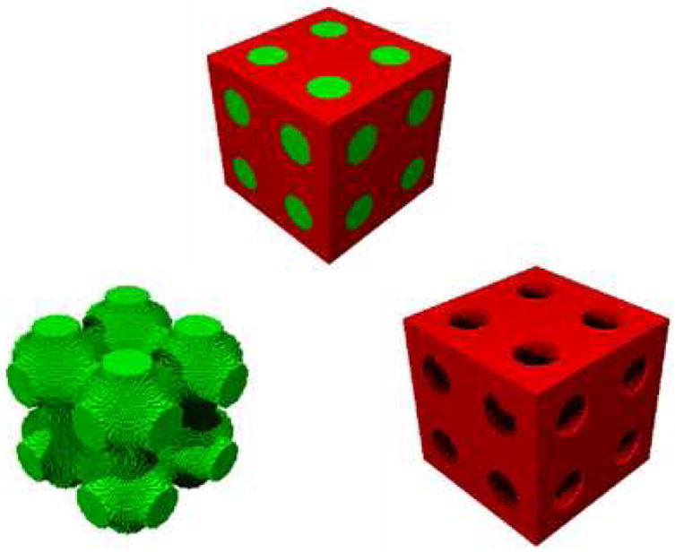
Two-phase composite whose interface is the Schwartz P minimal surface, which simultaneously optimizes heat and electrical conduction [81] or electrical conduction and elastic moduli [82]. The image at the top shows the two-phase composite. The bottom left image shows only one of the phases (green), which can be seen to be the Schwartz P minimal surface, and the bottom right image shows only the other phase (red).

9.3. The Far Out

Even more challenging and intriguing questions can be asked: Can we exploit the unique properties of normal stem cells [87] to control cancer (e.g., to deliver therapy to tumors or to have them compete with the tumor)? Can we use inverse optimization methods to design “hypothetical” cancers or stem cells with particular the cell-cell interactions to yield targeted behaviors and then make them in the lab? These “inverse” problems are motivated by their analog in statistical mechanics [88, 89, 90, 91]. In statistical mechanics, the “forward problem” is one in which a Hamiltonian (interaction potential) for a many-body system is specified and then structure of the system and its thermodynamics are predicted. By contrast, the “inverse” problem of statistical mechanics seeks to find the “optimal” interaction potential that leads spontaneously to a novel “targeted” structure (or behavior). We have discovered optimal interaction potentials that yield unusual or counterintuitive targeted ground (zero-temperature) states, e.g., low-coordinated diamond crystal [89] and disordered states [90] with only isotropic pair potentials (see Figure 21). Ground states are those many-particle configurations that arise as a result of slowly cooling a liquid to absolute zero temperature. The aforementioned obtained targeted ground states are so unusual because much of our experience involves ground states that are highly-coordinated crystal structures [91]. An extremely challenging and fascinating question is whether we can devise inverse optimization techniques to control cancer?

Figure 21.

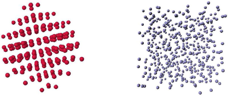
The ground-state structures for isotropic pair interaction potentials obtained via “inverse” optimization techniques discussed in the text. Left panel: A diamond-crystal ground state [89]. Right panel: A disordered ground state [90].

It is clear that theoretical methods based in the physical and mathematical sciences offer many different fruitful ways to contribute to tumor research. However, for this approach to be successful, intensive interactions with cell biologists, oncologists, radiologists, clinicians, physicists, chemists, engineers, and applied mathematicians are essential. Such an interdisciplinary approach appears to be necessary in order to control this deadly disease. This could be achieved most effectively if we could have an analog of the “Manhattan Project” in which there was a single facility with such an interdisciplinary team of scientists dedicated to this supreme achievement.

Figure 4.

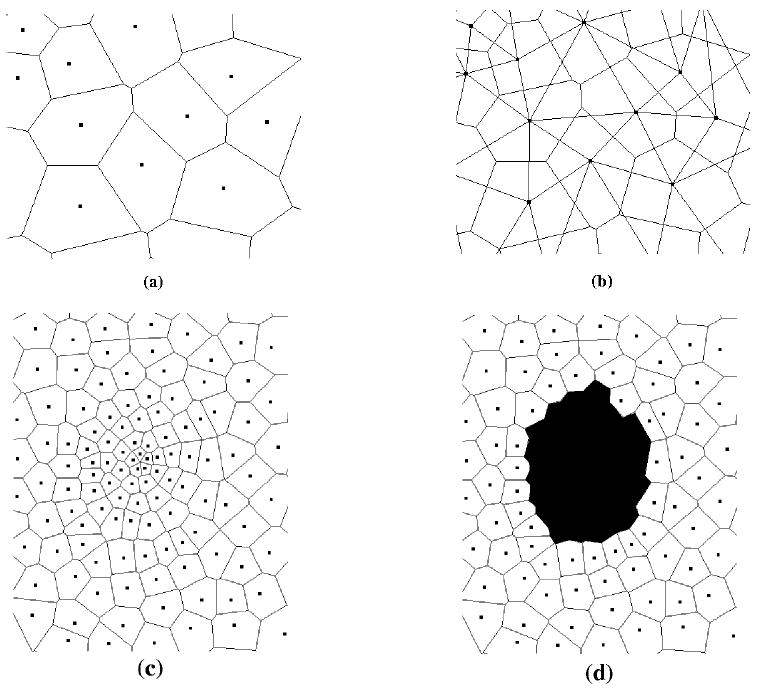
Two-dimensional space tiled into Voronoi cells, as adapted from Ref. [11]. Points represent sites and lines denote boundaries between cells. Figures (a) and (b) depict a very small section of a lattice. (a) shows the Voronoi cells, while (b) shows both the Voronoi cells, along with the Delaunay tessellation. Figures (c) and (d) show a more representative section of the lattice, with the variable density of sites evident. Panel (c) shows the entire lattice section, (d) shows the same section with the darkened cells representing a tumor.

Glossary

Neoplasm

A neoplasm is a synonym for a tumor

Glioma

A collection of tumors arising from the glial cells or their precursors in the central nervous system

Cellular automaton

A spatially and temporally discrete model that consists of a grid of cells, with each cell being in one of a number of predefined states. The state of a cell at a given point in time depends on the state of itself and its neighbors at the previous discrete time point. Transitions between states are determined by a set of local rules

Ising model

The Ising model is an idealized statistical-mechanical model of ferromagnetism that is based on simple local-interaction rules, but nonetheless lead to basic insights and features of real magnets, such as phase transitions with a critical point

Voronoi cell

Given a set of points, the Voronoi cell is the cell that is formed about an arbitrary point in the set by finding the region of space closer to that point than any other point in the system (Torquato, 2002)

Delaunay triangulation

Given a Voronoi graph (a set of Voronoi cells), the Delaunay graph is its dual that results from joining all pairs of sites that share a Voronoi face. If this graph consists of only simplices, the graph is called a Delaunay triangulation (Torquato, 2002)

Quiescent

A cell is considered quiescent if it is in the G0 phase of the cell cycle and is not actively dividing

Necrotic

A cell is considered necrotic if it has died due to injury or disease, such as abnormally low oxygen levels

References

- 1.Hanahan D, Weinberg RA. The hallmarks of cancer. Cell. 2000;100:57–70. doi: 10.1016/s0092-8674(00)81683-9. [DOI] [PubMed] [Google Scholar]
- 2.Crossa FR, Tinkelenberga AH. A potential positive feedback loop controlling cln1 and cln2 gene expression at the start of the yeast cell cycle. Cell. 1991;65:875–883. doi: 10.1016/0092-8674(91)90394-e. [DOI] [PubMed] [Google Scholar]
- 3.Deisboeck TS, Berens ME, Kansal AR, Torquato S, Rachamimov A, Louis DN, Chiocca EA. Patterns of self-organization in tumor systems: Complex growth dynamics in a novel brain tumor spheroid model. Cell Proliferat. 2001;34:115–134. doi: 10.1046/j.1365-2184.2001.00202.x. [DOI] [PMC free article] [PubMed] [Google Scholar]
- 4.Brand U, Fletcher JC, Hobe M, Meyerowitz EM, Simon1dagger R. Dependence of stem cell fate in arabidopsis on a feedback loop regulated by clv3 activity. Science. 2000;289:617–619. doi: 10.1126/science.289.5479.617. [DOI] [PubMed] [Google Scholar]
- 5.Kitano H. Cancer as a robust system: implications for anticancer therapy. Nature Reviews Cancer. 2004;4:227–235. doi: 10.1038/nrc1300. [DOI] [PubMed] [Google Scholar]
- 6.Chaplain MAJ, Sleeman BD. Modelling the growth of solid tumours and incorporating a method for their classification using nonlinear elasticity theory. J Math Biol. 1993;31:431–473. doi: 10.1007/BF00173886. [DOI] [PubMed] [Google Scholar]
- 7.Tracqui P, Cruywagen GC, Woodward DE, Bartoo GT, Murray JD, Alvord EC. A mathematical model of glioma growth: The effect of chemotherapy on spatio-temporal growth. Cell Proliferation. 1995;28:17–31. doi: 10.1111/j.1365-2184.1995.tb00036.x. [DOI] [PubMed] [Google Scholar]
- 8.Gatenby RA. Applications of competition theory to tumour growth: Implications for tumour biology and treatment. Eur J Cancer. 1996;32:722–726. doi: 10.1016/0959-8049(95)00658-3. [DOI] [PubMed] [Google Scholar]
- 9.Anderson ARA, Chaplain MAJ. Continuous and discrete mathematical models of tumor-induced angiogenesis. Bull Math Biol. 1998;60:857900. doi: 10.1006/bulm.1998.0042. [DOI] [PubMed] [Google Scholar]
- 10.Panetta JC. A mathematical model of drug resistance: Heterogeneous tumors. Mathematical Biosciences. 1998;147:41–61. doi: 10.1016/s0025-5564(97)00080-1. [DOI] [PubMed] [Google Scholar]
- 11.Kansal AR, Torquato S, Harsh GR, Chiocca EA, Deisboeck TS. Simulated brain tumor growth using a three-dimensional cellular automaton. J Theo Bio. 2000;203:367–382. doi: 10.1006/jtbi.2000.2000. [DOI] [PubMed] [Google Scholar]
- 12.Kansal AR, Torquato S, Chiocca EA, Deisboeck TS. Emergence of a subpopulation in a computational model of tumor growth. J Theo Bio. 2000;207:431–441. doi: 10.1006/jtbi.2000.2186. [DOI] [PubMed] [Google Scholar]
- 13.Schmitz JE, Kansal AR, Torquato S. A cellular automaton model of brain tumor treatment and resistance. J Theo Medicine. 2002;4:223–239. [Google Scholar]
- 14.McDougall SR, Anderson ARA, Chaplain MAJ, Sherrat JA. Mathematical modelling of flow through vascular networks: implications for tumor-induced angiogenesis and chemotherapy strategies. Bull Math Biol. 2002;64:673–702. doi: 10.1006/bulm.2002.0293. [DOI] [PubMed] [Google Scholar]
- 15.Alarcón T, Byrne HM, Maini PK. A multiple scale model for tumor growth. Multiscale Model Simul. 2005;3:440–475. [Google Scholar]
- 16.Cristini V, Frieboes HB, Gatenby R, Caerta S, Ferrari M, Sinek J. Morphological instability and cancer invasion. Clin Cancer Res. 2005;11:6772–6779. doi: 10.1158/1078-0432.CCR-05-0852. [DOI] [PubMed] [Google Scholar]
- 17.Frieboes HB, Zheng X, Sun Chung-Ho, Tromberg B, Gatenby R, Cristini V. An integrated computational/experimental model of tumor invasion. Cancer Res. 2006;66:1597–1604. doi: 10.1158/0008-5472.CAN-05-3166. [DOI] [PubMed] [Google Scholar]
- 18.Gevertz JL, Torquato S. Modeling the effects of vasculature evolution on early brain tumor growth. J Theo Bio. 2006;243:517. doi: 10.1016/j.jtbi.2006.07.002. [DOI] [PubMed] [Google Scholar]
- 19.Swanson KR, Rockne R, Rockhill JK, Alvord EC., Jr Combining mathematical modeling with serial mr imaging to quantify and predict response to radiation therapy in individual glioma patient. Neuro-Oncology. 2007;9:575. [Google Scholar]
- 20.Gevertz JL, Gillies G, Torquato S. Simulating tumor growth in confined heterogeneous environments. Physical Biology. 2008;5:036010. doi: 10.1088/1478-3975/5/3/036010. [DOI] [PubMed] [Google Scholar]
- 21.Gevertz J, Torquato S. Growing heterogeneous tumors in silico. Phys Rev E. 2009;80:051910. doi: 10.1103/PhysRevE.80.051910. [DOI] [PubMed] [Google Scholar]
- 22.Gerlee P, Anderson AR. Evolution of cell motility in an individual-based model of tumour growth. J Theor Biol. 2009;259:67–83. doi: 10.1016/j.jtbi.2009.03.005. [DOI] [PMC free article] [PubMed] [Google Scholar]
- 23.Ramis-Conde I, Chaplain MA, Anderson AR, Drasdo D. Multi-scale modelling of cancer cell intravasation: the role of cadherins in metastasis. Phys Bio. 2009;6:16008. doi: 10.1088/1478-3975/6/1/016008. [DOI] [PubMed] [Google Scholar]
- 24.Frieboes HB, Jin F, Chuang YL, Wise SM, Lowengrub JS, Cristini V. Three-dimensional multispecies nonlinear tumor growth- II: Tumor invasion and angiogenesis. J Theor Biol. 2010;264:1254–78. doi: 10.1016/j.jtbi.2010.02.036. [DOI] [PMC free article] [PubMed] [Google Scholar]
- 25.Byrne H. Dissecting cancer through mathematics: from the cell to the animal model. Nature Review. 2010;10:221–231. doi: 10.1038/nrc2808. [DOI] [PubMed] [Google Scholar]
- 26.Coffey DS. Self-organization, complexity and chaos: the new biology for medicine. Nat Med. 1998;4:882–885. doi: 10.1038/nm0898-882. [DOI] [PubMed] [Google Scholar]
- 27.Holland EC. Glioblastoma multiforme: the terminator. PNAS. 2000;97:6242–6244. doi: 10.1073/pnas.97.12.6242. [DOI] [PMC free article] [PubMed] [Google Scholar]
- 28.Wheeler CJ, Black KL, Liu G, Mazer M, Zhang X-X, Pepkowitz S, Goldfinger D, Ng H, Irvin D, Yu JS. Vaccination elicits correlated immune and clinical responses in i glioblastoma multiforme patients. Cancer Res. 2010;68:5955–5964. doi: 10.1158/0008-5472.CAN-07-5973. [DOI] [PubMed] [Google Scholar]
- 29.Holash J, Maisonpierre PC, Compton D, Boland P, Alexander CR, Zagzag D, Yancopoulos GD, Weigand SJ. Vessel cooption, regression, and growth in tumors mediated by angiopoietins and vegf. Science. 1999;284:1994–1998. doi: 10.1126/science.284.5422.1994. [DOI] [PubMed] [Google Scholar]
- 30.Brat DJ, Castellano-Sanchez AA, Hunter SB, Pecot M, Cohen C, Hammond EH, Devi SN, Kaur B, Van Meir EG. Pseudopalisades in glioblastoma are hypoxic, express extracellular matrix proteases, and are formed by an actively migrating cell popultion. Cancer Res. 2004;64:920–927. doi: 10.1158/0008-5472.can-03-2073. [DOI] [PubMed] [Google Scholar]
- 31.Singh SK, Clarke ID, Hide T, Dirks PB. Cancer stem cells in nervous system tissues. Oncogene. 2004;23:7267–7273. doi: 10.1038/sj.onc.1207946. [DOI] [PubMed] [Google Scholar]
- 32.Singh SK, Hawkins C, Clarke ID, Squire JA, Bayani J, Hide T, Mekelman RM, Cusimano MD, Dirks PB. Identification of human brain tumour initiating cells. Nature. 2004;432:396–401. doi: 10.1038/nature03128. [DOI] [PubMed] [Google Scholar]
- 33.Düchting W, Vogelsaenger T. Recent progress in modelling and simulation of three-dimensional tumor growth and treatment. Biosystems. 1985;18:79–91. doi: 10.1016/0303-2647(85)90061-9. [DOI] [PubMed] [Google Scholar]
- 34.Qi AS, Zheng X, Du CY, An BS. A cellular automaton model of cancerous growth. J Theor Biol. 1993;161:1–12. doi: 10.1006/jtbi.1993.1035. [DOI] [PubMed] [Google Scholar]
- 35.Smolle J, Stettner H. Computer simulation of tumour cell invasion by a stochastic growth model. J Theor Biol. 1993;160:63–72. doi: 10.1006/jtbi.1993.1004. [DOI] [PubMed] [Google Scholar]
- 36.Wasserman R, Acharya R, Sibata C, Shin KH. A patient-specific in vivo tumor model. Math Biosci. 1996;136:111–140. doi: 10.1016/0025-5564(96)00045-4. [DOI] [PubMed] [Google Scholar]
- 37.Steel GG, Peckham MJ. Exploitable mechanisms in combined radiotherapy-chemotherapy: The concept of additivity. Int J Rad Oncol. 1997;5:85–91. doi: 10.1016/0360-3016(79)90044-0. [DOI] [PubMed] [Google Scholar]
- 38.Berkman RA, Clark WC, Saxena A, Robertson JT, Oldfield EH, Ali IU. Clonal composition of glioblastoma multiforme. J Neurosurg. 1992;77:432–437. doi: 10.3171/jns.1992.77.3.0432. [DOI] [PubMed] [Google Scholar]
- 39.Coons SW, Johnson PC. Regional heterogeneity in the DNA content of human gliomas. Cancer. 1993;72:3052–3060. doi: 10.1002/1097-0142(19931115)72:10<3052::aid-cncr2820721030>3.0.co;2-7. [DOI] [PubMed] [Google Scholar]
- 40.Paulus W, Peiffer J. Intratumoral histologic heterogeneity of gliomas. a quantitative study. Cancer. 1989;64:442–447. doi: 10.1002/1097-0142(19890715)64:2<442::aid-cncr2820640217>3.0.co;2-s. [DOI] [PubMed] [Google Scholar]
- 41.Yung WA, Shapiro JR, Shapiro WR. Heterogeneous chemosensitivities of subpopulations of human glioma cells in culture. Cancer Res. 1982;42:992–998. [PubMed] [Google Scholar]
- 42.Nowell PC. The clonal evolution of tumor cell populations. Science. 1976;194:23–28. doi: 10.1126/science.959840. [DOI] [PubMed] [Google Scholar]
- 43.Loeb LA. Microsatellite instability: Marker of a mutator phenotype in cancer. Cancer Res. 1994;54:5059–5063. [PubMed] [Google Scholar]
- 44.Lengauer C, Kinzler KW, Vogelstein B. Genetic instabilities in human cancers. Nature. 1998;396:643–649. doi: 10.1038/25292. [DOI] [PubMed] [Google Scholar]
- 45.Heppner GH, Miller BE. Therapeutic implications of tumor heterogeneity. Bull Mathemat Biol. 1989;16:91–105. [PubMed] [Google Scholar]
- 46.Schnipper LE. Clinical implications of tumor cell heterogeneity. New Eng J Med. 1986;314:1423–1431. doi: 10.1056/NEJM198605293142206. [DOI] [PubMed] [Google Scholar]
- 47.Bredel M. Anticancer drug resistance in primary human brain tumors. Brain Research Reviews. 2001;35:161–204. doi: 10.1016/s0165-0173(01)00045-5. [DOI] [PubMed] [Google Scholar]
- 48.Endicott LC, Ling V. The biochemistry of the p-glycoprotein-mediated multidrug resistance. Annual Reviews in Biochemistry. 1989;58:137–171. doi: 10.1146/annurev.bi.58.070189.001033. [DOI] [PubMed] [Google Scholar]
- 49.German UA. P-glycoprotein–a mediator of multidrug resistance in tumour cells. European Journal of Cancer. 1996;32:927–944. doi: 10.1016/0959-8049(96)00057-3. [DOI] [PubMed] [Google Scholar]
- 50.Poppenborg H, Munstermann G, Knopfer MM, Hotfilder M, Wolff JEA. C6 cross-resistant to cisplatin and radiation. Anticancer Research. 1997;17:2073–2077. [PubMed] [Google Scholar]
- 51.Chadhary PM, Roninson IB. Induction of multidrug resistance in human cells by transient exposure to different chemotherapeutic drugs. Journal of the National Cancer Institute. 1993;85:632–639. doi: 10.1093/jnci/85.8.632. [DOI] [PubMed] [Google Scholar]
- 52.Gekeler V, Beck J, Noller A, Wilisch A, Frese G, Neumann M, Handgretinger R, Ehninger G, Probst H, Niethammer D. Drug-induced changes in the expression of mdr-associated genes - investigations on cultured cell lines and chemotherapeutically treated leukemias. Annals of Hematology. 1994;69:S19–S24. doi: 10.1007/BF01757350. [DOI] [PubMed] [Google Scholar]
- 53.Gerweck LE, Kornblinth PL, Burlett P, Wang J, Sweigert S. Radiation sensitivity of cultured glioblastoma cells. Radiology. 1977;125:231–241. doi: 10.1148/125.1.231. [DOI] [PubMed] [Google Scholar]
- 54.Kayama T, Yoshimoto T, Fujimoto S, Sakurai Y. Intratumoral oxygen pressure in malignant brain tumors. Journal of Neurosurgury. 1991;74:55–59. doi: 10.3171/jns.1991.74.1.0055. [DOI] [PubMed] [Google Scholar]
- 55.Zhang W, Hara A, Sakai N, Andoh T, Yamada H, anf PH, Gutin YN, Kornblinth PL. Radiosensitization and inhibition of deoxyribonucleic acid repair in rat glioma cells by long term treatment with 12-o-tetradecanoylphorbol 13-acatate. Neurosurgury. 1993;32:432–437. doi: 10.1227/00006123-199303000-00015. [DOI] [PubMed] [Google Scholar]
- 56.Holash J, Wiegand SJ, Yancopoulos GD. New model of tumor angiogenesis: dynamic balance between vessel regression and growth mediated by angiopoietins and vegf. Oncogene. 1999;18:5356–5362. doi: 10.1038/sj.onc.1203035. [DOI] [PubMed] [Google Scholar]
- 57.Maisonpierre CS, Suri C, Jones PF, Bartunkova S, Wiegand SJ, Radziejewski C, Compton D, McClain J, Aldrich TH, Papadlopoulous N, Daly TJ, Davis S, Sato TN, Yancopoulos GD. Angiopoietin-2, a natural antagonist for tie2 that disrupts in vivo angiogenesis. Science. 1997;277:55–60. doi: 10.1126/science.277.5322.55. [DOI] [PubMed] [Google Scholar]
- 58.Secomb TW, Hsu R, Beamer NB, Coull BM. Theoretical simulation of oxygen transport to brain by networks of microvessels: effects on oxygen supply and demand on tissue hypoxia. Microcirculation. 2000;7:237–247. [PubMed] [Google Scholar]
- 59.Giese A, Manfred W. Glioma invasion in the central nervous system. Neurosurgery. 1996;39:235–252. doi: 10.1097/00006123-199608000-00001. [DOI] [PubMed] [Google Scholar]
- 60.Visted T, Enger PO, Lund-Johansen M, Bjerkvig R. Mechanisms of tumor cell invasion and angiogenesis in the central nervous system. Front in Bioscience. 2003;8:289–304. doi: 10.2741/1026. [DOI] [PubMed] [Google Scholar]
- 61.Kansal AR, Torquato S. Globally and locally minimal weight branched tree networks. Physica A. 2001;301:601–619. [Google Scholar]
- 62.Torquato S. Random Heterogeneous Materials: Microstructure and Macroscopic Properties. Springer-Verlag; New York: 2002. [Google Scholar]
- 63.Helmlinger G, Netti PA, Lichtenbeld HC, Melder RJ, Jain RK. Solid stress inhibits the growth of multicellular tumor spheroids. Nat Biotechnol. 1997;15:778–83. doi: 10.1038/nbt0897-778. [DOI] [PubMed] [Google Scholar]
- 64.Sun T, Meakin P, Jossang T. Minimum energy dissipation model for river basin geometry. Phys Rev E. 1994;49:48654872. doi: 10.1103/physreve.49.4865. [DOI] [PubMed] [Google Scholar]
- 65.RodriguezIturbe I, Rinaldo A. Fractal River Basins. Cambridge University Press; Cambridge: 1997. [Google Scholar]
- 66.West GB, Brown JH, Enquist BJ. A general model for the origin of allometric scaling laws in biology. Science. 1997;276:122126. doi: 10.1126/science.276.5309.122. [DOI] [PubMed] [Google Scholar]
- 67.Haouari M, Dror M, Chaouachi J. Generalized spanning trees. Eur J Oper Res. 2000;120:583–592. [Google Scholar]
- 68.Torquato S, Kim IC, Cule D. Effective conductivity, dielectric constant, and diffusion coefficient of digitized composite media via first-passage-time-equations. J Appl Phys. 1999;85:1560–1572. [Google Scholar]
- 69.Lee SB, Kim IC, Miller CA, Torquato S. Random-walk simulation of diffusion-controlled processes among static traps. Phys Rev B. 1989;39:11833–11839. doi: 10.1103/physrevb.39.11833. [DOI] [PubMed] [Google Scholar]
- 70.Torquato S. Diffusion and reaction among traps: some theoretical and simulation results. J Stat Phys. 1991;65:1173–1207. [Google Scholar]
- 71.Quintanilla J, Torquato S. New bounds on the elastic moduli of suspensions of spheres. J Appl Phys. 1995;77:4361–4372. [Google Scholar]
- 72.Torquato S. Exact epression for the effective elastic tensor of disordered composites. Phys Rev Lett. 1997;79:681–685. [Google Scholar]
- 73.Kim IC, Torquato S. Effective conductivity of suspensions of hard spheres by Brownian motion simulation. J Appl Phys. 1991;69:2280–2289. [Google Scholar]
- 74.Gibiansky LV, Torquato S. Thermal expansion of isotropic multiphase composites and polycrystals. J Mech Phys of Solids. 1997;45:1223–1252. [Google Scholar]
- 75.Torquato S, Lu B. Rigorous bounds on the fluid permeability: effect of polydispersivity in grain size. Phys Fluids A. 1990;2:487–491. [Google Scholar]
- 76.Torquato S. Effective electrical conductivity of two-phase disordered composite media. J Appl Phys. 1985;58:3790–3797. [Google Scholar]
- 77.Sen AK, Torquato S. Effective electrical conductivity of two-phase disordered anisotropic composite media. Phys Rev B. 1989;39:4504–4516. doi: 10.1103/physrevb.39.4504. [DOI] [PubMed] [Google Scholar]
- 78.Gevertz JL, Torquato S. A novel three-phase model of brain tissue microstructure. Plos Comput Bio. 2008;4:e100052. doi: 10.1371/journal.pcbi.1000152. [DOI] [PMC free article] [PubMed] [Google Scholar]
- 79.Torquato S, Pham DC. Optimal bounds on the trapping constant and permeability of porous media. Phys Rev Lett. 2004;92:255505. doi: 10.1103/PhysRevLett.92.255505. [DOI] [PubMed] [Google Scholar]
- 80.Sigmund O, Torquato S. Design of materials with extreme thermal expansion using a three-phase topology optimization method. J Mech Phys Solids. 1997;45:1037–1067. [Google Scholar]
- 81.Torquato S, Hyun S, Donev A. Multifunctional composites: optimizing microstructures for simultaneous transport of heat and electricity. Phys Rev Lett. 2002;89:266601. doi: 10.1103/PhysRevLett.89.266601. [DOI] [PubMed] [Google Scholar]
- 82.Torquato S, Donev A. Minimal surfaces and multifunctionality. Proc R Soc Lond A. 2004;460:1849–1856. [Google Scholar]
- 83.Torquato S. Optimal design of heterogeneous materials. Ann Rev Mater Res. 2010;40:101–129. [Google Scholar]
- 84.Jung Y, Torquato S. Fluid permeabilities of triply periodic minimal surfaces. Phys Rev E. 2005;92:255505. doi: 10.1103/PhysRevE.72.056319. [DOI] [PubMed] [Google Scholar]
- 85.Gevertz JL, Torquato S. Mean survivial times of absorbing triply periodic minimal surfaces. Phys Rev E. 2009;80:011102. doi: 10.1103/PhysRevE.80.011102. [DOI] [PubMed] [Google Scholar]
- 86.Dingli D, Chalub FACC, Santos FC, Van Segbroeck S, Pacheco JM. Cancer phenotype as the outcome of an evolutionary game between normal and malignant cells. Brit J Cancer. 2009;101:1130–1136. doi: 10.1038/sj.bjc.6605288. [DOI] [PMC free article] [PubMed] [Google Scholar]
- 87.Reya T, Morrison SJ, Clarke MF, Weissman1 IL. Stem cells, cancer, and cancer stem cells. Nature. 2001;414:105–111. doi: 10.1038/35102167. [DOI] [PubMed] [Google Scholar]
- 88.Rechtsman M, Stillinger FH, Torquato S. Optimized interactions for targeted self-assembly: application to honeycomb lattice. Phys Rev Lett. 2005;95:228301. doi: 10.1103/PhysRevLett.95.228301. [DOI] [PubMed] [Google Scholar]
- 89.Rechtsman M, Stillinger FH, Torquato S. Synthetic diamond and wurtzite structures self-assemble with isotropic pair interactions. Phys Rev E. 2007;75:031403. doi: 10.1103/PhysRevE.75.031403. [DOI] [PubMed] [Google Scholar]
- 90.Batten RD, Stillinger FH, Torquato S. Novel low-temperature behavior in classical many-particle systems. Phys Rev Lett. 2009;103:050602. doi: 10.1103/PhysRevLett.103.050602. [DOI] [PubMed] [Google Scholar]
- 91.Torquato S. Inverse optimization techniques for targeted self-assembly. Soft Matter. 2009;5:1157–1174. [Google Scholar]