

Abstract
A method for estimating dipole preserving and polarization consistent (DPPC) charges is described, which reproduces exactly the molecular dipole moment as well as the local, atomic hybridization dipoles determined from the corresponding wave function, and can yield accurate molecular polarization. The method is based on a model described by Thole and van Duijnen and a new feature is introduced in the DPPC model to treat molecular polarization. Thus, the DPPC method offers a convenient procedure to describe molecular polarization in applications using semiempirical models and ab initio molecular orbital theory with relatively small basis functions such as 6-31+G(d,p) or without inclusion of electron correlation; these methods tend to underestimate molecular polarizability. The trends of the DPPC partial atomic charges are found to be in good accord with those of the CM2 model, a class IV charge analysis method that has been used in a variety of applications. The DPPC method is illustrated to mimic the correct molecular polarizability in a water dimer test case and in water-halide ion complexes using the explicit polarization (X-Pol) potential with the AM1 Hamiltonian.
1. Introduction
Partial atomic charges are not physical observables that can be measured experimentally,1 but the concept is extremely useful in our qualitative understanding of structure and reactivity and in sophisticated applications such as biomolecular simulations. In practice, they are obtained according to the specific need and there are many ways of deriving partial charges.2 In this article, we describe a method to produce atomic partial charges that can be used in combined quantum mechanical and molecular mechanical (QM/MM)3 or mixed QM/QM potentials,4–5 or in the explicit polarization (X-Pol)6–10 quantal force field for biomolecular simulations.11 In this article, we make use of semiempirical methods that are computationally efficient and capable of yielding excellent molecular dipole moments,12–14 although we emphasize that any quantum mechanical models can be employed. Storer et al.15 classified the way by which partial charges are derived into four categories, including (i) extraction from experimental data, (ii) population analysis of the molecular wave function,16–17 (iii) property fitting18–20 such as the electrostatic potential obtained from quantum mechanical calculations21–24 or from experiments,1 and (iv) semiempirical mapping that transforms the population charges to best reproduce the experimental dipole moments.15,25 Each category has its own strengths and weaknesses and they have been lucidly discussed in the past.2,15,26 One particular approach is the Mulliken population analysis17 which is often criticized for its lack of consistency, especially using large basis sets. Nevertheless, the Mulliken population analysis enjoys its simplicity, which can provide an indication of the relative charge separation in a molecular system.25 Mulliken population charges have been used as the reference point in the class IV charge models,15,25,27 which has been adopted in combined QM/MM simulations.28
Thole and van Duijnen19 described a population analysis that preserves the dipole moment of the molecule by distributing partial atomic charges with the constraint that the molecular dipole moment is identical to that determined from the molecular wave function. The original method of Thole and van Duijnen only utilizes molecular geometry about which the charge reassignment was made;19 however, as the complexity of a molecule increases, it is difficult to choose a proper weighting function to take into account the properties of functional groups. Subsequently, Swart et al.29 extended that approach to preserve atomic multipole moments that are derived from atomic charge densities using density functional theory. Although the latter approach is very appealing especially in calculations using high quality electron densities with augmented basis functions, it is less useful in situations when relatively small basis functions are used such as 6-31+G(dp) or the minimal basis in semiempirical models.30–31 In the later case, Mulliken population analysis in fact provides an adequate starting point, as shown by Truhlar and Cramer et al. in their development of class IV charge models15,25 to map partial charges that can yield molecular dipole moments in good agreement with experiments. This strategy is particularly attractive for applications using semiempirical methods such as the Austin model 1 (AM1)12 or the recently developed parameterization model 6 (PM6)13 because they have been parameterized to reproduce experimental dipole moments.
Our goal is to use partial atomic charges to represent the molecular electrostatic moments of the molecular wave function of individual fragments in solution or in a macromolecular system in combined QM/MM,3 multilayer QM/QM,4–5 and the X-Pol quantal force field.7,11 The procedure described by Thole and van Duijnen19 and later revised by Swart et al.19,29 meet this criterion. In this article, we present a method for deriving partial atomic charges from semiempirical Hamiltonians (or ab initio methods) by preserving the molecular dipole moment determined from the corresponding wave function exactly. Rather than redistributing partial atomic charges completely as was done in ref 29, we use the Mulliken charge as a reference state, and treat only the hybridization components in the dipole calculation for charge redistribution based on atomic electronegativity. The method is applicable both to neutral molecules and charged systems, independent of the origin of the coordinate system. Significantly, not only the qualitative features of the Mulliken population analysis are retained in this procedure, but also the local hybridization dipole components as well as the total molecular dipole moment from the wave function is preserved.12–13
In addition, we incorporate Thole’s interaction dipole (TID)32 polarization method into the dipole preserving scheme to ensure that the generally weakly polarized semiempirical wave function can also adequately represent molecular polarization. Together, the present method preserves molecular dipole moment from the wave function and ensures consistent molecular polarization; the partial atomic charges derived from semiempirical Hamiltonians can be suitable for dynamics simulations of macromolecular systems and modeling of protein-ligand interactions using multilayer QM/QM potentials4–5 or a fully quantal (X-Pol) force field.6,8,11
In this paper we first summarize the dipole-preserving algorithm employed in our implementation, which is a modified approach used by Swart et al.29 Then, we describe the incorporation of a molecular polarization consistent procedure, which is a new contribution of this work. We call this approach the dipole preserving and polarization consistent (DPPC) charge analysis. We choose a set of molecules that were used in the work of Storer et al.15 in the development of the CM1A charges based on the AM1 Hamiltonian to illustrate the performance and qualitative trends of the DPPC charges in the gas phase because both methods are developed with the aim to produce molecular dipole moments in good agreement with experiment. The Class IV charge models of Cramer and Truhlar are derived based on empirical fit to experimental dipole moments of a database, whereas the present DPPC method is an analytical procedure without empirical parameters except a weighting function for charge distribution. Excluding nitrile compounds, the semiempirical AM1, PM3, and PM6 models, and the corresponding DPPC charges, can yield molecular dipole moments in excellent agreement with experiments with standard errors of about 0.3 D for this database, which is comparable or smaller than the standard errors of the CM1A method (or the latter CM2 model). In a subsequent study of condensed phase systems, including liquids and solutions, the ability to recover correct molecular polarization will be tested in statistical mechanical Monte Carlo and molecular dynamics simulations, employing the explicit polarization (X-Pol)8,11 quantal force field.7
2. Method
2.1. Background
The Mulliken population charge of atom k is partitioned from the density matrix P as
| (1) |
where Zk is the nuclear charge, P is the one-electron density matrix and S is the overlap matrix of the basis functions. The superscript “o” in eq 1 is to indicate that the Mulliken population charges will be used as the reference state for deriving the DPPC charges. Although the method is general, here, we focus on sermiempirical methods based on the NDDO approximation,30 in which the quantum mechanical (QM) molecular dipole moment is determined as a sum of two contributing terms:33
| (1) |
where DMP is the contribution from Mulliken charges, and Dhyb is the one-center s and p hybridization contribution. The Mulliken population (MP) dipole is simply:
| (2) |
where N is the number of atoms, and {rk; k = 1, ⋯, N} are the atomic positions. The s-p hybridization component is written as:
| (3) |
where (Psp)k is a diagonal matrix with the densities of the s and p orbitals on atom k, and Rk is the corresponding dipole integral. It is well-known that the one-center hybridization polarization terms make substantial contributions to the total molecular dipole moment.33 As a result, DMP is not expected to yield good agreement with experimental dipole.
Our goal is to incorporate additionally distributed charges, called residual charges, to exactly reproduce the hybridization contribution in eq 3 such that the sum of the residual and Mulliken population charges will preserve the local, atomic (hybridization) point dipoles and the total molecular dipole moment from the full density of the molecular wave function. In our approach, the hybrid polarization dipole is defined as the optimization target in the residual charge distributing procedure:19
| (4) |
It is important to emphasize that the net molecular charge is represented by the Mulliken population charges, while the hybridization term Dhyb has no net charge contributions. Consequently, ΔD in eq 4 is translationally and rotationally invariant both for neutral and ionic systems such that the charge preserving method describe in this paper is applicable both to neutral molecules and to ions. As shown in eq 3, the total polarization dipole can be written as a sum of atomic contributions; thus, the optimization target can also be expressed in terms of atomic components:
| (5) |
Of course, there are other ways of decomposing the total molecular dipole, or generally, multipole moments, into atomic components. For example, the atomic multipole moments can be obtained from atomic electron densities fitted to reproduce the total molecular electron density (either from the wave function in a QM calculation or from X-ray diffraction).1 Typically, an auxiliary basis of Slater orbitals is used to represent the atomic density (as in DFT calculations), from which atomic multipole moments are derived. Although this method is very appealing, a very large basis set must be used to obtain a good fit to the molecular electron density, which is not particularly useful for semiempirical models employing a minimal basis. Further, the fitted auxiliary densities generally do not reproduce the molecular dipole and multipole moments computed directly from the electronic structure method. Consequently, additional auxiliary functions and constraints must be imposed.29
The density fitting procedure was used in the multipole derived charge introduced by Swart et al.,29 who described an algorithm that preserves atomic multipole moments at any order. The approach employed in our study is similar to that method,19,29 but the procedure and details are different. In the method of Swart et al., the atomic charges are obtained by fully redistributing the residual charges to all atomic centers with the constraint that the atomic or molecular moments are reproduced. In the present study, the Mulliken population charges are kept as the zeroth order reference, from which the error in the Mulliken population charge, ΔDi, relative to the exact quantum mechanical moment is defined as the fitting target. Thus, the redistributed charges may be regarded as perturbations to the Mulliken population charge. In the following, we limit our discussion to dipole preservation, although the procedure can be analogously applied to moments at any order.29
2.2. Locally distributed dipole-preserving charges (DPC)
For each atomic (i.e., s-p hybridization polarization) dipole to be preserved, ΔDi, where i = 1,⋯, N, we wish to assign a set of atomic charges, called residual charges, distributed to atomic centers in the molecule such that they reproduce the target hybridization dipole exactly:
| (6) |
where is the residual atomic charge on atom k, associated with the atomic dipole ΔDi located on atom i. We seek to obtain a set of residual charges that make the smallest perturbation to the Mulliken population charges under the constraints that the net change is zero, thereby preserving the net molecular charge.
| (7) |
The total atomic charge of atom k is thus the sum of the Mulliken population charge and the residual charges due to the preservation of all atomic hybridization dipole moments:
| (8) |
The residual charges associated with the dipole moment ΔDi (i = 1,⋯, N), are obtained by using the Lagrange multiplier method, in which we minimize the charge variation subject to the constraints of eqs 6 and 7, i.e., that the residual dipole, or the error in the Mullike population dipole is exactly corrected and the total charge variation is zero. Thus, for atom i,
| (9) |
where α and β are the Lagrangian multipliers, and is a set of weighting functions (vide infra) that controls the way that the charge redistribution is accomplished.
The residual charges should be dominantly distributed to sites closest to the dipole ΔDi on atom i that they aim to reproduce. In addition, it is important to be proportionally distributed according to the relative electron-withdrawing ability of different atoms. For example, for acetaldehyde, CH3CH=O, one expects to enhance the partial charges of oxygen and carbon, rather than dominantly on the methyl and hydrogen atoms. The weighting function may be constructed based on the relative values of the off-diagonal matrix elements of the density matrix that contribute to the residual dipole moment, or devised according to the relative Mulliken charges. We choose a weighting function dependent on the relative electronegativity and the interatomic distance as follows:
| (10) |
where λ is a constant, chosen to be close to 1.0 Å−2, ηi and ηk are the Pauling electronegativity of atoms i and k, respectively. A weighting function without the use of electronegativity has been used previously19,29 and tested, which distributes charges equally to atomic sites with the same distance from the reference atom i without discriminating their relative electron-withdrawing powers.
Minimization of the Lagrangian (eq 9) by variation with respect to yields
| (11) |
where the superscript T indicates a matrix (vector) transpose. The solution of this equation, whose details are given in the Appendix, yields a final expression for the charge increments associated with the atomic hybridization dipole ΔDi:
| (12) |
where the various terms are defined as follows:
| (13) |
| (14) |
| (15) |
2.3. Molecular polarization consistent charges
The procedure outlined above also offers a convenient way to correct the errors in computed molecular polarization in semiempirical methods, which prevent a good description of hydrogen bonding interactions. Generally, it is necessary to use large basis functions with electron correlations to accurately predict molecular polarizability in electronic structure calculations. Further, higher order polarization terms are ignored in the treatment of intermolecular interactions in condensed phase simulations.
Let αSE be the molecular polarizability tensor of an approximate quantum chemical model such as AM1 or PM6, and αtarget be the target molecular polarizability tensor from experiment, from a high-level quantum mechanical calculation, or from an empirical dipole polarization model that has been shown to be able to yield a good prediction of molecular polarizability. Our goal is to derive a set of polarized DPPC charges to correct the error due to αSE and to reproduce the molecular polarization described by αtarget.
In the presence of an external electrostatic field, we write the total molecular dipole moment DSE as a sum of the permanent dipole in the absence of the external field and the induced dipole moment :
| (16) |
where the induced dipole moment is related to the external electrostatic field E(R) due to all other molecules, R, in the condensed phase by
| (17) |
Accurate calculation of molecular polarizability requires a large basis set with augmented functions as well as correlation. Typically, the computed molecular polarizabilities from semiempirical methods are too small in comparison with experiments. For example, the scalar polarizability for water is only 0.5 Å3 using AM1 and other semiempirical modes, whereas the experimental value is 1.47 Å3. Thus, if the current semiempirical models are used directly to model biomolecular systems or aqueous solution where polarization effects are important, intermolecular interactions due to polarization are also poorly treated.7 The error in the computed induced dipole moment due to the use of a small molecular polarizability can be expressed as follows:
| (18) |
which can be recast in terms of the computed induced dipole moment:
| (19) |
Here, ΔΔDind is the error due to the use of a weakly polarized model (from semiempirical or ab initio quantum calculations with small basis sets without including electron correlation), which can be included as part of the dipole-preservation target in the charge redistribution scheme described in Section 2.2. In this case, both the intrinsic, gas-phase dipole moment and the correct induced dipole moment due to an external electrostatic field from the environment will be preserved. This approach is called the DPPC method. We further assume (vide infra) that the total induced dipole moment can be decomposed into atomic contributions; here, we note that there is no unique way of decomposing molecular polarizability into atomic contributions, but abundant data exist, showing that atomic and group additivity schemes can be used to estimate the total molecular polarizability.34–35 Then, the Lagrangian optimization constraint of eq 5 for atomic point dipoles is replaced by
| (20) |
It should be emphasized that both the hybridization and induction polarization in eq 20 are obtained using the polarized wave function in the presence of the instantaneous external field E(R). The second term, which is the error in the computed molecular induced dipole, becomes zero in the absence of the external electrostatic field. In this case, the DPPC analysis is simply reduced to a dipole preserving charge (DPC) calculation outlined in the previous section. Obviously, if the quantum mechanical method used can accurately describe molecular polarization, the second term in eq 20 is also negligible since Δα is close to zero. Using the current semiempirical models, which describe molecular polarization rather poorly, we can, with eq 20, obtain a set of atomic partial charges that preserve the molecular dipole moment along with the extra induced dipole moment not adequately represented by the original wave function in condensed phase simulations.
The remaining task is to present a procedure so that only atomic parameters are needed to describe molecular polarization in the presence of an external field. To this end, we adopt another Thole’s contribution,32 the interacting dipole (TID) polarization model, which has been adopted, at least conceptually, in many polarizable force fields currently being developed.36–41 One remarkable feature of the Thole interacting dipole model is that isotropic atomic parameters that depend only on atomic numbers are used, but excellent agreement with experimental or high-level quantum mechanical results can be obtained on anisotropic molecular polarizabilities.32 A recent parameter set was reported by van Duijnen and Swart,42 and our own investigation confirmed that essentially the same atomic parameters were optimized using a much larger set of compounds in the fitting procedure (unpublished data; J. Pu and J. Gao, 2008). In the TID model,32 the total molecular polarizability can be conveniently decomposed into atomic site contributions,38,42 well suited for the present purposes.
Specifically, the TID molecular polarizability is given as follows:38,42
| (21) |
where the Greek letter subscripts specify a Cartesian coordinate (x, y or z), is an element of the molecular polarizability tensor, αTID is a diagonal matrix of isotropic atomic polarizabilities (the atomic parameters in the TID model),32,37,42 ) is the second-rank atomic interaction tensor (see eq 6 of ref 38), and the superscripts i and j run over atoms in the molecule. In the TID model, the molecular polarizability tensor is completely determined given a set of isotropic atomic polarizability and its geometry. It provides one of the most physical theories on molecular polarization that bridges electronic structure and classical models.
The atomic components of the total molecular polarizability tensor at atom i are defined by summing over the second summation in eq 21,34,38,42 which is
| (22) |
The ith mean atomic polarizability can be approximated as the average value of the three principal polarizability components determined by eq 22, .34,42 If we assume that the relative atomic contribution to the total molecular polarizability is the same in the semiempirical method as that of the TID model, eq 19 can be simplified as
| (23) |
Eqs 12, 20 and 23 provide a general approach that links a set of atomic polarizabilities (which have proven to be very good for describing molecular polarization)42 and a given QM model to yield a set of dipole and polarization preserving charges that may be used in association with the explicit polarization (X-Pol)11 potential to represent interfragment interactions or in multilayer QM/QM calculations.5
3. Rationale
The class IV charge models (CM1 through CM4, or simply CMx)15,43–44 have been shown to be useful for obtaining partial atomic charges, capable of yielding molecular dipole moments in excellent agreement with experiment. The CMx charges have been used as the fundamental electrostatic input to develop the accompanying solvation models (SMx) for prediction of solvent effects,43–44 and the method has been adopted in combined QM/MM simulations of chemical and enzymatic reactions.28 Thus, it provides a good standard for comparison with the partial charges derived from the present DPPC method since the latter is also developed based on the principle to reproduce molecular dipole moments. Unlike the philosophy adopted in the CM1-CM4 charge models,15,27 the present DPPC approach does not require a training set of molecular dipole moments to parameterize the model. The DPPC analysis is an optimization procedure to yield partial atomic charges that exactly reproduce the molecular dipole moment from the corresponding quantum mechanical wave function. However, it is important to use a quantum chemical model, either semiempirical, ab initio or density functional theory, that can yield good results on molecular dipole moment in comparison with experiments. Therefore, we use the training set of molecules in the parameterization of the CM1 charges15 to illustrate that the current semiempirical models,12–13,45 consequently, the DPPC charges, can produce molecular dipole moments as accurately as the CMx charges.
The CM1 database consisting of 185 neutral molecules were selected from several compilations of experimental dipole moments with relative precision within ±0.02 D.15 Storer et al. described the construction of this database as “mainly monofunctional organic molecules that have been chosen to isolate possible systematic deficiencies in the AM1 and PM3 wave functions.”15 For H, C, N and O containing compounds, the database includes 12 alcohols, 8 esters and lactones, 16 carbonyl compounds, 9 acids, 10 ethers, 13 amines, 3 amides, 7 imines and aromatics, and 24 mono and multifunctional nitrile compounds. In addition, 83 compounds are included to cover halogen, silicon and sulfur containing compounds. The root mean square (RMS) errors for CM1-AM1 charges from ref 15 are duplicated in Table 1, along with that of the recently developed PM6 model. Overall, AM1 and PM3, respectively, have RMS errors of ±0.45 and ±0.47 D for the 185 compounds, while the RMS errors in the dipole moments computed using the CM1 and CM2 charges are ±0.25 and ±0.22 D. AM1 and PM3 perform very poorly for the nitriles with average errors greater than 1.0 D and 0.8 D, respectively. If the 24 cyano compounds are excluded, the errors in the semiempirical models are reduced to ±0.34 D for AM1, compared with the CM1A charge model of ±0.24 D. If we only consider the H, C, N and O containing compounds, which are the most relevant to biomolecular systems, excluding the nitriles, the AM1 error in dipole moment is ±0.24 D, even smaller than that of ±0.29 D from the CM1A charge model and ±0.32 D from CM2 charges. If the Mulliken charges are directly used to estimate molecular dipole moments, the errors are very large, in the range of ±0.8 to ±0.9 D.15 Overall, the comparison suggests that the current semiempirical models12–13,45 are excellent for estimating molecular dipole moments despite their inconsistent performance on relative energies.
Table 1.
Root mean square errors in the computed dipole moment (debye) from experimental data for compounds used in the parameterization of the class IV charge model (CM1A).
| compounds | No. | PM3 | PM6 | AM1 | CM1A | CM2(AM1)a |
|---|---|---|---|---|---|---|
| Alcohols | 12 | 0.61 | 0.43 | 0.17 | 0.21 | 0.25 (0.17) |
| Esters, lactones | 8 | 0.30 | 0.38 | 0.25 | 0.24 | 0.33 (0.18) |
| Carbonyls | 16 | 0.42 | 0.43 | 0.25 | 0.18 | 0.32 (0.17) |
| Acids | 9 | 0.23 | 0.41 | 0.31 | 0.41 | 0.58 (0.16) |
| Ethers | 10 | 0.19 | 0.45 | 0.17 | 0.18 | 0.14 (0.20) |
| Amines | 13 | 0.25 | 0.64 | 0.25 | 0.17 | 0.14 (0.17) |
| Amides | 3 | 0.52 | 0.26 | 0.15 | 0.69 | 0.23 (0.23) |
| Imines | 7 | 0.35 | 0.38 | 0.28 | 0.43 | 0.34 (0.31) |
| Nitriles | 24 | 0.78 | 0.30 | 1.00 | 0.16 | 0.29 (0.21) |
| H, C, N, O without nitriles | 78 | 0.38 | 0.46 | 0.24 | 0.29 | 0.32 |
| All H, C, N, O | 102 | 0.47 | 0.43 | 0.47 | 0.29 | 0.31 (0.21) |
| Other compounds | 83 | 0.47 | 0.40 | 0.19 | ||
| All compounds | 185 | 0.47 | 0.37b | 0.45 | 0.25 | (0.22) |
Values in parentheses were obtained using the HF/MIDI! geometry in ref. 25.
4. Computational Details
Molecular geometries for the H, C, O, and N subset of the CM1-database have been optimized using the corresponding semiempirical model to determine the DPPC charges. We have also implemented and recomputed the CM2 charges, from which the CM2 dipole moments were estimated. Note that the CM2 parameters were optimized using geometries optimized with the HF/MIDI! method, thereby the small difference between the present CM2 dipoles and those reported in ref 46.
The DPPC method is not without parameters since a weighting function is used to redistribute the residual partial charges associated the constrained dipole target. The parameters include the distance damping factor λ in eq 6, which is chosen to be unity, and the Pauling electronegativity for each element (H: 2.20; C: 2.55; N: 3.04; and O: 3.44). To preserve the desired molecular polarizability using the Thole interaction dipole model, isotropic atomic polarizability parameters will be needed; these parameters have been optimized and reported by van Duijnen and Swart.42 In addition, the DPPC method involves the inversion of a 3×3 geometrical matrix δi, which could be singular in certain situations such as a planer molecule. In this case, we adopted the eigenvalue smoothing approach to ensure numerical stability. Thus, the three eigenvalues of δi are perturbed with a small increment of θ = 10−5 to avoid singularity:19
| (24) |
where ω is one of the three eigenvalus of δi and ωmax is the largest eigenvalue.
5. Illustrative examples
We first present the dipole preserving charges (DPC) in the gas phase for the compounds in the CM1 database in Sections 5.1 through 5.6. Then, the effect of including polarization consistency in the DPPC method is discussed next.
5.1. Water and alcohols
The Mulliken population, DPC and CM2 atomic charges for water and methanol determined using AM1, PM3 and PM6 models (note that there are no CM2 parameters for the PM6 method) are shown in Figure 1. The absolute values of standard Mulliken population charges are generally too small in comparison with the typical values used in the force fields for biomolecular simulations and that needed in the generalized Born-base solvation models. The dipole moments computed using the Mulliken population charges are substantially smaller than the results from the corresponding wave function and experiments. The DPC charge for oxygen of water is enhanced from −0.38 e to −0.65 e, which is slightly smaller than the CM2 charge of −0.71. The latter over-estimates the molecular dipole moment proportionally. For alcohols, the oxygen partial charge is increased by about 0.2 a.u. similar to that from the empirical fit in the CM2 model. As in the CM2 model, the partial charges on atoms of the alkyl group are not significantly affected by the Lagrangian minimization procedure, and it is of interest to point out that the hydrogen atoms attached to a carbon can have different partial charges, depending on their conformational orientation, whereas in they are typically assigned with an identical partial charge in force fields such as OPLS47 and CHARMM,48 independent on the instantaneous environment. Overall, the mean unsigned errors in the computed dipole moments for the 12 alcohol compounds are 0.13 D for the AM1-DPC charges, 0.33 D for PM3, 0.36 D for PM6, and 0.20 D for CM2, while the RMS errors are 0.17, 0.61, 0.43, and 0.25 D, respectively.
Figure 1.
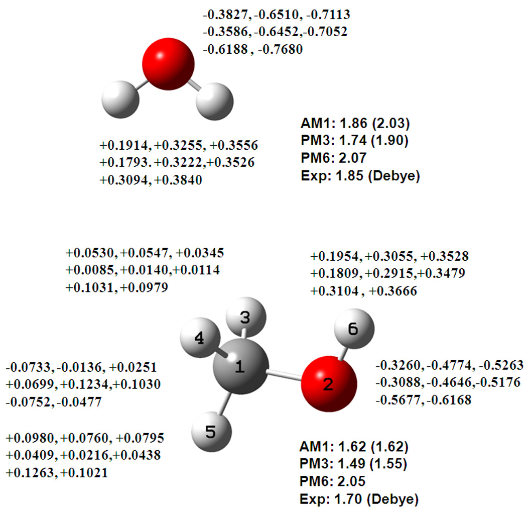
Computed dipole moments and partial atomic charges for water and methanol from Mulliken population (first), the DPC method (second), and the CM2 model (third), using the AM1 (top line), PM3 (middle line), and PM6 (lower line) models. Partial charges are determined by Mulliken population analysis given first, followed by the DPPC charges and CM2 charges. The first row for each atom lists charges from the AM1 method, the second row shows charges from the PM3 model, and the third row depicts charges from the PM6 Hamiltonian. All charges are given in electron charge unit. Computed dipole moments from each model are given in Debye followed by values determined with the CM2 charges, and the experimental dipole value is listed last. This convention is used throughout Figures 1 to 5.
5.2. Esters and lactones
Eight compounds are included for the esters and lactones functional groups in the CM1 database. The RMS errors in the computed dipole moments for the DPC model are 0.25, 0.30, 0.38 D from the AM1, PM3 and PM6 models, compared to the CM2 error of 0.33 D using the AM1 wave function. To illustrate the qualitative trend, the partial atomic charges are depicted in Figure 2 for methyl acetate. The positive charge on the carbonyl carbon and the negative charge on the ester and carbonyl oxygen atoms are significantly enhanced in the DPC model and the results are in excellent accord with the CM2 method.
Figure 2.
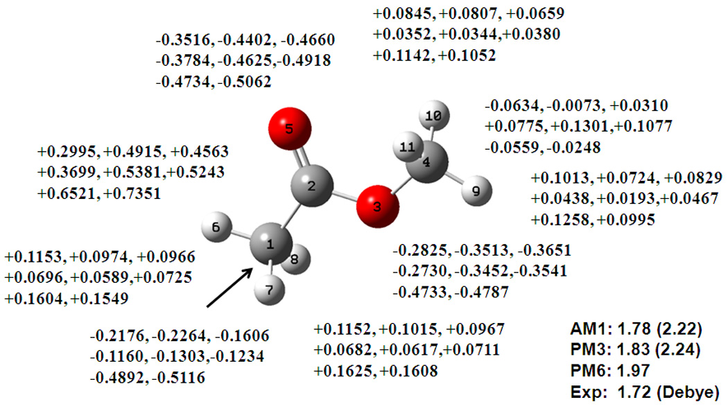
Computed dipole moment and partial atomic charges for methy acetate from Mulliken population (first), the DPC method (second), and the CM2 model (third), using the AM1 (top line), PM3 (middle line), and PM6 (lower line) models. See also Figure 1 caption.
5.3. Carbonyl compounds
A total of sixteen carbonyl compounds, ranging from aldehyde and ketones to cyclic and conjugated carbonyls are included, which have RMS errors of 0.25, 0.42 and 0.43 D using AM1, PM3, and PM6, respectively. The CM2 error using AM1 is 0.32 D, somewhat larger than that of the original CM1A charges (0.21 D). The partial atomic charges from the DPC and CM2 models are shown in Figure 3 for 2-butanone. Although the carbonyl oxygen and carbon net charges are increase by about 0.1 a.u., they are still smaller than that used in the CHARMM force field,48 which are −0.51 and +0.51 a.u. for oxygen and carbon, respectively. The force field charges are designed for condensed-phase simulations that include effective polarization effects. It would be interesting to examine the DPC performance in solution and biomolecular simulations. The CM2 charges are slightly more enhanced than the DPC charges for the carbonyl group, and the general patterns of the partial atomic charges from both models (DPC and CM2) are very similar.
Figure 3.
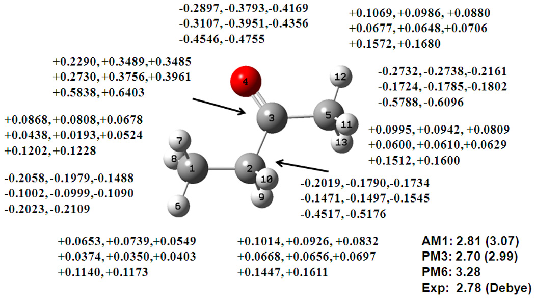
Computed dipole moment and partial atomic charges for 2-butanone from Mulliken population (first), the DPC calculation (second), and the CM2 model (third), using the AM1 (top line), PM3 (middle line), and PM6 (lower line) models. See also Figure 1 caption.
5.4. Carboxylic acids and ethers
Although the average errors for the nine carboxylic acids appear to be large from all methods, this is somewhat skewed by the two acrylic acid configurations. Nevertheless, the results are reasonable with RMS errors of 0.31, 0.23, and 0.41 D for AM1, PM3, and PM6, respectively, and it is 0.58 D from the CM2 charges. The ether compounds are very well described by all models with RMS errors less than 0.2 D, except PM6, which has a relatively large RMS deviation of 0.45 D.
5.5. Amines and ammonia
Although the molecular dipole moments are very well reproduced by the AM1 and PM3 models, with an average error of 0.25 D in comparison with experiments, it is well known that the charge separation between nitrogen and attached (polar) hydrogen atoms are not well described. The later PM6 model performs much worse overall, with an RMS error of 0.64 D. The main problem is that the negative charge on the amino nitrogen atom is small in comparison with that optimized for condensed phase simulations. The redistribution of the hybridization polarization charges in the DPC model enhances the nitrogen negative charges of alkyl amines and ammonia significantly, in good accord with the corresponding CM2 charges. This is illustrated for methylamine and ammonia in Figure 4. However, the planer aniline group is still under estimated in the DPC charges, suggesting that further improvements may be needed to circumvent the singularity issue in the geometrical matrix inversion.
Figure 4.
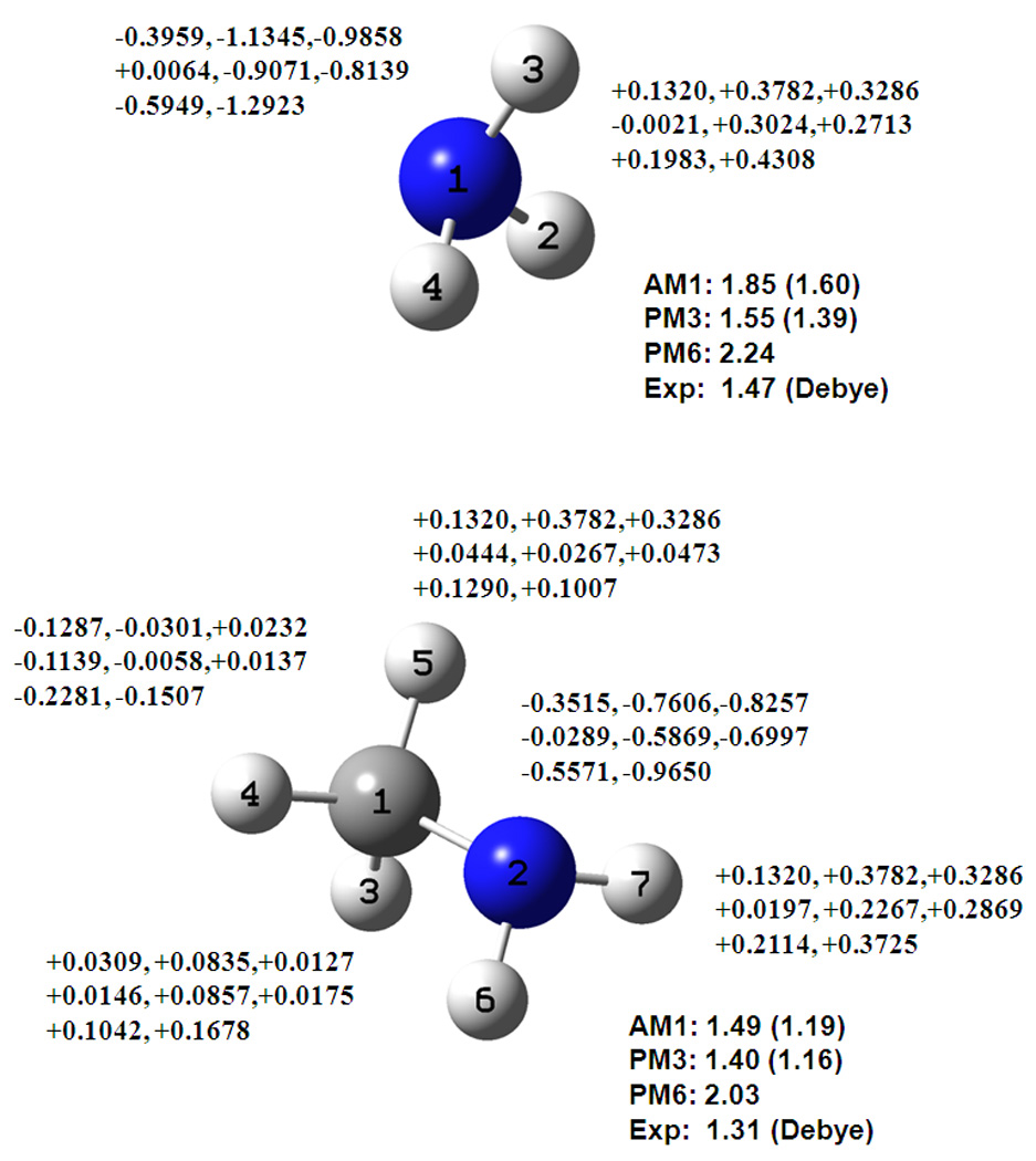
Computed dipole moments and partial atomic charges for ammonia and methylamine from Mulliken population (first), the DPC analysis (second), and the CM2 model (third), using the AM1 (top line), PM3 (middle line), and PM6 (lower line) models. See also Figure 1 caption.
5.6. Amides and imines
The atomic charges for acetamide and N-methylformamide are shown in Figure 5. Atomic charges on the nitrogen atom in amides and imines from the DPC model are significantly smaller than those mapped with the CM2 model. In the latter case, more than −0.4 a.u. of negative charge is placed on the nitrogen atom, along with proportional increase in the positive charges on the hydrogen atoms attached to the amide and imine nitrogen atoms and the carbonyl or imine carbon atoms. The partial charges on the amide nitrogen atom used in the OPLS47 and CHARMM48 force fields are −0.57 and −0.47 a.u., respectively. Although the force field charges take into account average polarization effects in aqueous solution, the magnitude is significantly smaller than the CM2 charges. It is expected that the DPC charges will be enhanced in aqueous solution due to polarization effects. Interestingly, despite the large range of negative charge on the amide nitrogen atom from different models, the overall molecular dipole moments are not significantly affected, reflecting the arbitrariness of partial charge assignment.
Figure 5.
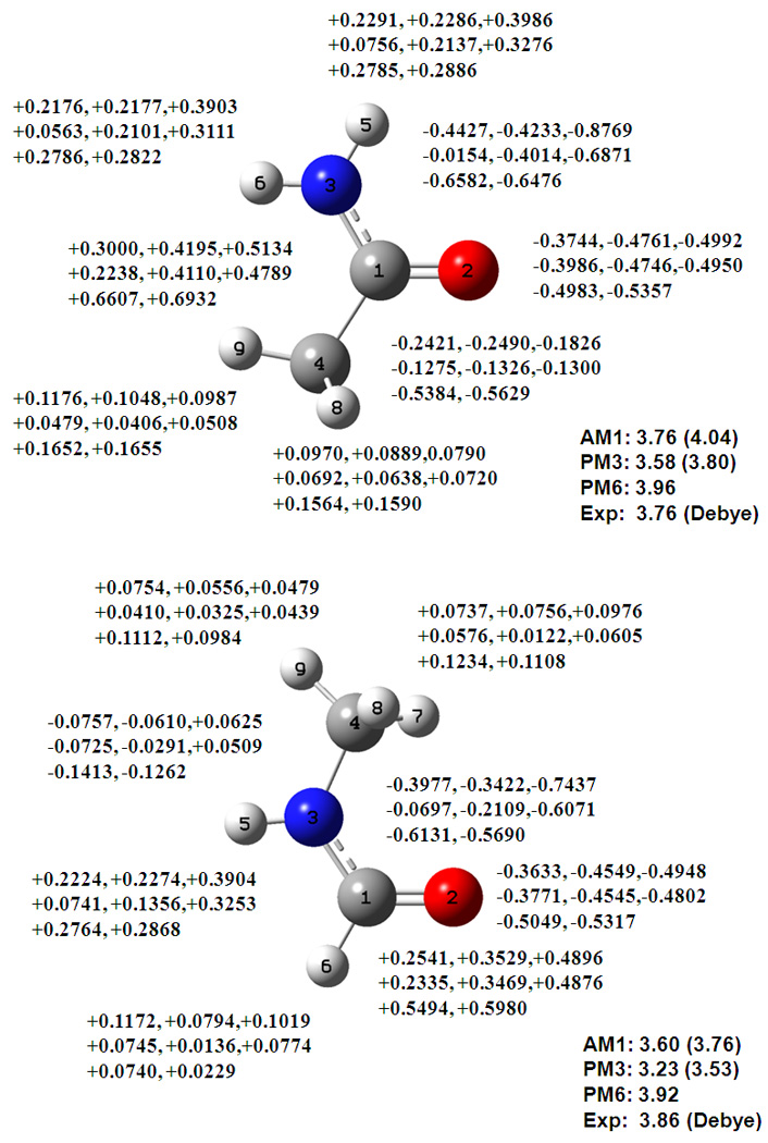
Computed dipole moments and partial atomic charges for acetamide and N-methylformamide from Mulliken population (first), the DPC method (second), and the CM2 model (third), using the AM1 (top line), PM3 (middle line), and PM6 (lower line) models. See also Figure 1 caption.
5.7. Polarization
Although the current semiempirical models can yield an excellent estimate of molecular dipole moment in the gas phase, polarization effects are severely underestimated, preventing these methods to be applied to model biomolecular interactions such as solvation and ligand-protein binding. The DPPC method is designed to reproduce the correct electronic polarization with a better description of the induced dipole moment in the presence of an external electric field. To properly test this approach, statistical mechanical Monte Carlo and molecular dynamics simulations of solutions are required, which is beyond the scope of this paper, but will be carried out subsequently. Here, we examine the polarization preservation capability of the DPPC model by considering the interaction profile of two water molecules along the minimum interaction energy path (Figure 6), and the bimolecular complexes of one water with a fluoride ion and with a chloride ion.
Figure 6.
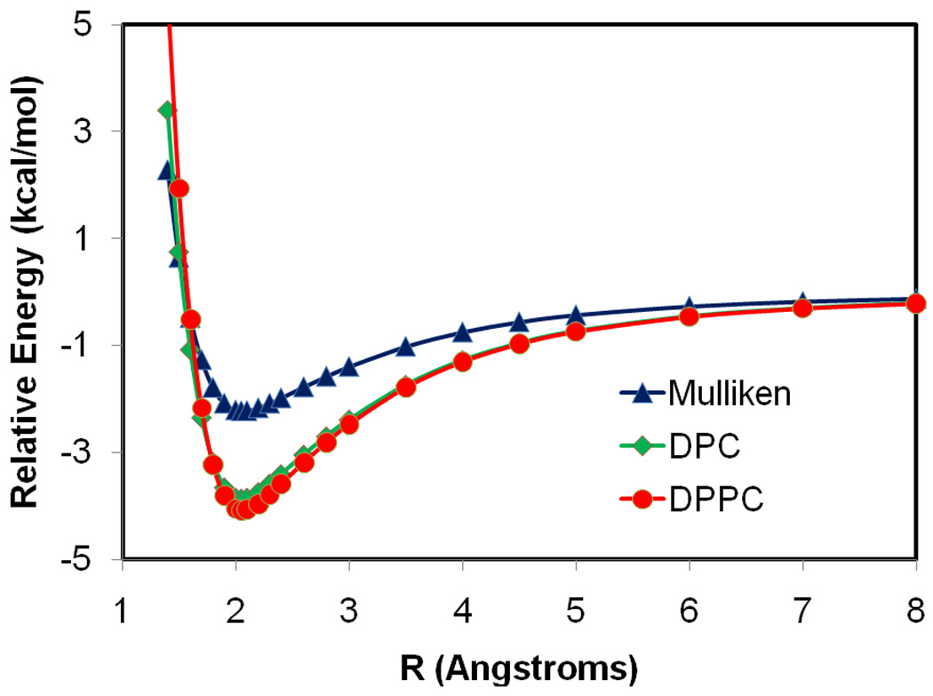
Interaction energy profiles for a water dimer complex as a function of the donor hydrogen and acceptor oxygen distance. The structural arrangement of the dimer complex is depicted by the inlay in the figure. The X-Pol potential with the AM1 Hamiltonian is used with each water molecule treated as a separate fragment. In the present calculation, a value of 2.0 was used for the semiempirical α parameter in QM/MM type integrals,50 and the long-range dispersion interactions modeled by a Lennard-Jones term was not included. The Coulomb interactions between the two water fragments are determined by the X-Pol theory using the self-consistently optimized Mulliken population charges in blue, the dipole preserving charges (DPC) in green, and the dipole preserving and polarization consistent (DPPC) charges in red.
We use the X-Pol potential with the AM1 model in the present calculation,6 in which the molecular orbitals are block-localized within each monomer space. The system is represented by a two fragments,6–10 in which charge transfer effects are not included.49 First, the induced dipole moment for each water is determined by subtracting the “permanent” (i.e., gas-phase) dipole moment of water from that of the polarized monomer wave functions optimized from the X-Pol method. Then, the errors for the atomic induced dipoles, , in each water monomer from the AM1 Hamiltonian are estimated according to eq 23, using the Thole interaction dipole model.42 The induced dipole error together with the hybridization polarization is used to derive the polarized DPPC charges, which are included in SCF optimization of the X-Pol wave function.
The X-Pol interaction energies from the AM1 dipole preserving model (DPC) only and from the full DPPC charges are compared in Figure 6. The Mulliken population charges are too small to adequately represent the Coulomb potential from the original (AM1) wave function. These charges are significantly enhanced to preserve the dipole moment of the individual water molecules that are polarized in the presence of the electrostatic field of the other monomer. Thus, the binding energy is lowered by 1.6 kcal/mol (from −2.2 to −3.8 kcal/mol) using the DPC charges in the X-Pol(AM1) potential. The DPPC model yields stronger hydrogen bonding interactions (−4.1 kcal/mol) than the DPC model alone, due to correction of dipole polarization effects. At the interaction minimum, the binding energy from DPPC model is 6% greater than that with polarization preservation contributions. The partial atomic charges at the optimal geometry are shown in Figure 7. The Thole interacting dipole model yields a molecular polarizability identical to the experimental value for water; the partial charge on the acceptor oxygen atom is enhanced by 0.04 e units in going from the AM1 model (DPC charges) to the correctly polarized model (DPPC). Note that the X-Pol potential constructed from monomer block-localized molecular orbitals does not include charge transfer energy between the two monomers; thus, the total interaction energy is smaller than high-level ab initio results. In addition, the present calculations did not include the long-range dispersion interactions modeled by Lennard-Jones terms.6–7 Charge transfer and exchange repulsion can be explicitly incorporated into the X-Pol theory.49
Figure 7.
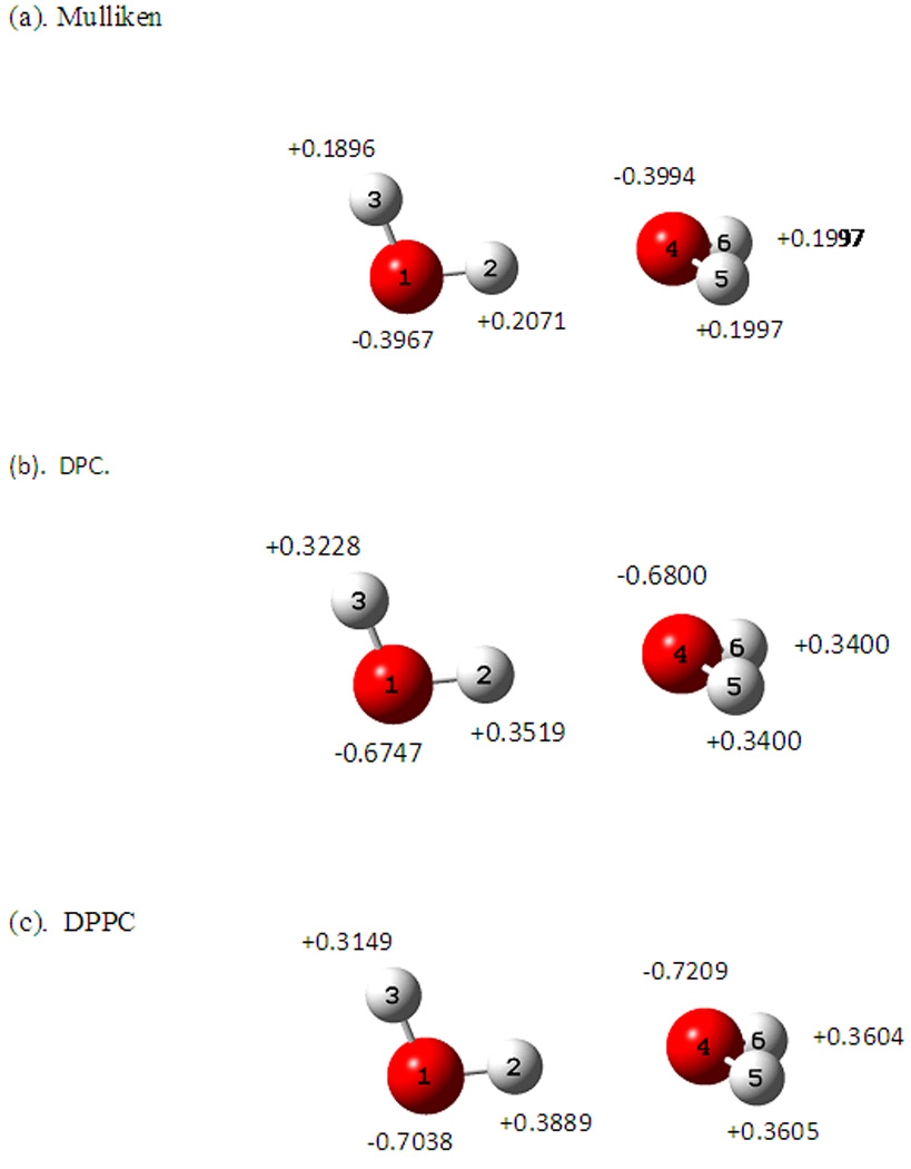
Equilibrium partial charges at the optimized dimer configuration, determined from the fully polarized monomer wave functions by the electrostatic field of the other water molecule using (a) Mulliken population analysis, (b) dipole preserving charge only, and (c) the full dipole preserving and polarization consistent analysis.
The polarization effect is further examined by placing a negative charge at distances of 2.049 and 1.550 Å from one of the hydrogen atoms of water at an angle of about 152° from oxygen (Figure 8), which mimics bimolecular hydrogen bonding complexes with a chloride ion and with a fluoride ion, respectively. There is no net polarization effect on the anion in the present minimum basis set representation of the full shell halogen ions and there is no charge transfer between water and the ion in this analysis, so only the wave function of the water molecule is polarized. Clearly, the dipole preserving feature (DPC) is important in charge estimation in comparison with the Mullike population analysis (Figure 8). Importantly, the inclusion of polarization consistency in the DPPC procedure to mimic the Thole interaction dipole polarizability, which is identical to that of the experimental value, further enhances the atomic charge separation by as much as 0.13 and 0.17 |e| units on the donor hydrogen atom for the chloride and fluoride ion complexes, respectively (Figure 8). Concomitantly, the interaction energies are enhanced from −13.9 to −15.4 kcal/mol for the chloride ion complex, and from −20.2 to −20.7 kcal/mol for the fluoride ion complex. Apparently, there are some saturation effects in dipole polarization since the probe ion is very close to bonding distance where the neglect of charge transfer effects is no longer a good approximation in the X-Pol model. In the latter case, if the water structure is allowed to relax, the AM1 model yields a hydroxide and hydrogen fluodride complex instead.
Figure 8.
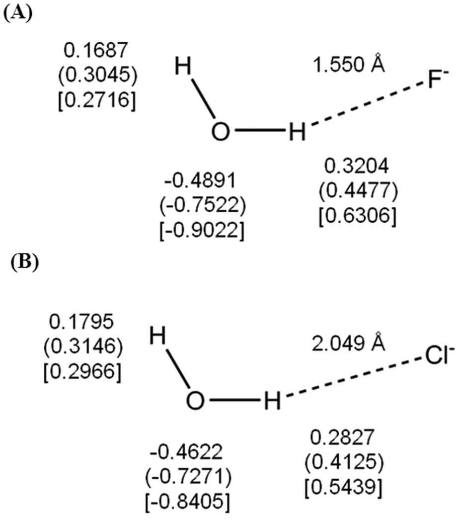
Computed partial atomic charges (a.u.) on the water molecule in (A) HOH…Cl− and (B) HOH…F− bimolecular complexes, in which the water geometry is held as that in the gas phase from AM1 optimization. The Mulliken population charges are given first, followed by the dipole preserving charge (DPC) in parentheses and the dipole preserving and polarization consistent (DPPC) charges in square brackets. The ion charges are negative one in the present minimum basis set representation using the AM1 model.
6. Conclusions
In the present study, we describe a method for estimating atomic partial charges, in which dipole moment from the corresponding quantum mechanical calculation is exactly preserved and the molecular polarizability is consistently incorporated. The method is called the dipole preserving and polarization consistent (DPPC) charge method. The dipole preservation approach has an origin from the work of Thole and van Duijnen;19 the new features of the DPPC model include charge redistribution based on relative atomic electronegativity and the treatment of molecular dipole polarization, consistent with the experimental or theoretical molecular polarizability. The latter is typically underestimated in semiempirical methods and in ab initio molecular orbital theory without inclusion of electron correlation. It was emphasized that the semiempirical models such as AM1, PM3 and PM6 can yield excellent results on molecular dipole moments in comparison with experiment, making these methods well suited for the DPPC analysis. The standard errors on the computed dipole moments from these semiempirical methods are similar to that determined using the well-parameterized Class IV charge models that have been successfully used in a variety of applications.
Using the database designed in the optimization of the CM1 model, excluding nitrile compounds that are not adequately treated by the semiempirical models, we show that the trends of the DPPC partial atomic charges are in good accord with those obtained from the CM2 model (using AM1). Furthermore, it was illustrated that the DPPC method can effectively introduce enhanced electronic polarization to mimic the correct molecular polarizability in a water dimer test case as well as in water-halogen ion bimolecular complexes using the X-Pol potential with AM1 Hamiltonian. One main difference between the present DPPC method and other charge models is that the DPPC partial charges reproduce the local (hybridization) and molecular dipole moments exactly, whereas partial atomic charges derived from electrostatic potential fitting procedure are known to have difficulties for atoms in the interior of a large molecule such as a protein. The DPPC analysis can also be coupled with combined QM/MM or QM/QM simulations to derive polarization consistent charges for use in empirical force fields.
Supplementary Material
Acknowledgments
This work was supported in part by the National Institutes of Health (RC1 GM091445) and the National Science Foundation (CHE09-57162).
Appendix. Derivation of Equation 12
We start with for the charge distribution over all N atoms in the molecule, , that preserves the atomic dipole ΔDi,
| (A1) |
The total charge variation, by definition, is
| (A2) |
where the total weight Wi and the weighted average coordinate associated with the dipole ΔDi have been defined in eqs 11 and 12, respectively. Similarly, the total residual (dipole-preserving and polarization-correction) dipole is
| (A3) |
Multiply both sides of eq A1 by <r>i from the right side, we obtain
| (A4) |
Subtract eq A4 from A3 to yield
| (A5) |
where we have used the definition for the matrix δi (eq 10). Multiplying both sides by the inverse matrix of δi we obtain
| (A6) |
Obviously,
| (A2) |
Since
| (A7) |
we separate the result term by term and obtain
| (A8) |
Footnotes
Supporting Information Available: Partial atomic charges for H, C, N and O containing compounds derived using the DPPC charge analysis and the CM2 model with the AM1 Hamiltonian. This material is available free of charge via the Internet at http://pubs.acs.org.
References
- 1.Coppens P. X-ray charge densities and chemical bonding. Chester, England: Oxford University Press; 1997. [Google Scholar]
- 2.Bachrach S. In: Rev. Comput. Chem. Lipkowitz KB, Boyd DB, editors. Vol. 5. Weinheim: VCH; 1994. [Google Scholar]
- 3.Gao J, Xia X. Science. 1992;258:631. doi: 10.1126/science.1411573. [DOI] [PubMed] [Google Scholar]
- 4.Hratchian HP, Parandekar PV, Raghavachari K, Frisch MJ, Vreven T. J. Chem. Phys. 2008;128:034107. doi: 10.1063/1.2814164. [DOI] [PubMed] [Google Scholar]
- 5.Parandekar PV, Hratchian HP, Raghavachari K. J. Chem. Phys. 2008;129:145101. doi: 10.1063/1.2976570. [DOI] [PubMed] [Google Scholar]
- 6.Gao J. J. Phys. Chem. B. 1997;101:657. [Google Scholar]
- 7.Gao J. J. Chem. Phys. 1998;109:2346. [Google Scholar]
- 8.Xie W, Gao J. J. Chem. Theory Comput. 2007;3:1890. doi: 10.1021/ct700167b. [DOI] [PMC free article] [PubMed] [Google Scholar]
- 9.Xie W, Song L, Truhlar DG, Gao J. J. Chem. Phys. 2008;128 doi: 10.1063/1.2936122. 234108/1. [DOI] [PMC free article] [PubMed] [Google Scholar]
- 10.Song L, Han J, Lin YL, Xie W, Gao J. J. Phys. Chem. A. 2009;113:11656. doi: 10.1021/jp902710a. [DOI] [PMC free article] [PubMed] [Google Scholar]
- 11.Xie W, Orozco M, Truhlar DG, Gao J. J. Chem. Theory Comput. 2009;5:459. doi: 10.1021/ct800239q. [DOI] [PMC free article] [PubMed] [Google Scholar]
- 12.Dewar MJS, Zoebisch EG, Healy EF, Stewart JJP. J. Am. Chem. Soc. 1985;107:3902. [Google Scholar]
- 13.Stewart JJP. J. Mol. Model. 2007;13:1173. doi: 10.1007/s00894-007-0233-4. [DOI] [PMC free article] [PubMed] [Google Scholar]
- 14.Tuttle T, Thiel W. Phys. Chem. Chem. Phys. 2008;10:2159. doi: 10.1039/b718795e. [DOI] [PubMed] [Google Scholar]
- 15.Storer JW, Giesen DJ, Cramer CJ, Truhlar DG. J Comput.-Aided Mol. Des. 1995;9:87. doi: 10.1007/BF00117280. [DOI] [PubMed] [Google Scholar]
- 16.Lowdin P-O. J. Chem. Phys. 1950;18:365. [Google Scholar]
- 17.Mulliken RS. J. Chem. Phys. 1964;61:20. [Google Scholar]
- 18.Hall D, Williams DE. Acta Crystallogr. 1975;A 31:56. [Google Scholar]
- 19.Thole BT, Vanduijnen PT. Theor. Chim. Acta. 1983;63:209. [Google Scholar]
- 20.Sternberg U, Koch FT, Mollhoff M. J. Comput. Chem. 1994;15:524. [Google Scholar]
- 21.Singh UC, Kollman PA. J. Comput. Chem. 1984;5:129. [Google Scholar]
- 22.Luque FJ, Illas F, Orozco M. J. Comput. Chem. 1990;11:416. [Google Scholar]
- 23.Momany FA. J. Phys. Cem. 1978;82:592. [Google Scholar]
- 24.Gao J, Luque FJ, Orozco M. J. Chem. Phys. 1993;98:2975. [Google Scholar]
- 25.Li J, Zhu T, Cramer CJ, Truhlar DG. J. Phys. Chem. A. 1998;102:1820. [Google Scholar]
- 26.Coppens P. Angew. Chem. Int. Ed. 2005;44:6810. doi: 10.1002/anie.200501734. [DOI] [PubMed] [Google Scholar]
- 27.Kalinowski JA, Lesyng B, Thompson JD, Cramer CJ, Truhlar DG. J. Phys. Cem. A. 2004;108:2545. [Google Scholar]
- 28.Acevedo O, Jorgensen WL. Acc. Chem. Res. 2010;43:142. doi: 10.1021/ar900171c. [DOI] [PMC free article] [PubMed] [Google Scholar]
- 29.Swart M, Van Duijnen PT, Snijders JG. J. Comput. Chem. 2001;22:79. [Google Scholar]
- 30.Pople JA, Santry DP, Segal GA. J. Chem. Phys. 1965;43:S129. [Google Scholar]
- 31.Stewart JJP. J. Comput.-Aided Mol. Des. 1990;4:1. doi: 10.1007/BF00128336. [DOI] [PubMed] [Google Scholar]
- 32.Thole BT. Chem. Phys. 1981;59:341. [Google Scholar]
- 33.Pople JA, Segal GA. J. Chem. Phys. 1965;43:S136. [Google Scholar]
- 34.Applequist J, Carl JR, Fung K-K. J. Am. Chem. Soc. 1972;94:2952. [Google Scholar]
- 35.Miller KJ. J. Am. Chem. Soc. 1990;112:8533. [Google Scholar]
- 36.Gao J, Habibollazadeh D, Shao L. J. Phys. Chem. 1995;99:16460. [Google Scholar]
- 37.Xie W, Pu J, MacKerell AD, Jr., Gao J. J. Chem. Theory Comput. 2007;3:1878. doi: 10.1021/ct700146x. [DOI] [PMC free article] [PubMed] [Google Scholar]
- 38.Xie W, Pu J, Gao J. J. Phys. Chem. A. 2009;113:2109. doi: 10.1021/jp808952m. [DOI] [PMC free article] [PubMed] [Google Scholar]
- 39.Ren P, Ponder JW. J. Comput. Chem. 2002;23:1497. doi: 10.1002/jcc.10127. [DOI] [PubMed] [Google Scholar]
- 40.Ren P, Ponder JW. J. Phys. Chem. B. 2003;107:5933. [Google Scholar]
- 41.Harder E, Anisimov VM, Vorobyov IV, Lopes PEM, Noskov SY, MacKerell AD, Jr., Roux B. J. Chem. Theory Comput. 2006;2:1587. doi: 10.1021/ct600180x. [DOI] [PubMed] [Google Scholar]
- 42.van Duijnen PT, Swart M. J. Phys. Chem. A. 1998;102:2399. [Google Scholar]
- 43.Li J, Zhu T, Cramer CJ, Truhlar DG. J. Phys. Chem. A. 2000;104:2178. [Google Scholar]
- 44.Chamberlin AC, Cramer CJ, Truhlar DG. J. Phys. Chem. B. 2006;110:5665. doi: 10.1021/jp057264y. [DOI] [PubMed] [Google Scholar]
- 45.Stewart JJP. J. Comp. Chem. 1989;10:209. [Google Scholar]
- 46.Zhu T, Li J, Hawkins GD, Cramer CJ, Truhlar DG. J. Chem. Phys. 1998;109:9117. [Google Scholar]
- 47.Jorgensen WL, Tirado-Rives J. J. Am. Chem. Soc. 1988;110:1657. doi: 10.1021/ja00214a001. [DOI] [PubMed] [Google Scholar]
- 48.MacKerell AD, Jr., Bashford D, Bellott M, Dunbrack RL, Evanseck JD, Field MJ, Fischer S, Gao J, Guo H, Ha S, Joseph-McCarthy D, Kuchnir L, Kuczera K, Lau FTK, Mattos C, Michnick S, Ngo T, Nguyen DT, Prodhom B, Reiher WE, III, Roux B, Schlenkrich M, Smith JC, Stote R, Straub J, Watanabe M, Wiorkiewicz-Kuczera J, Yin D, Karplus M. J. Phys. Chem. B. 1998;102:3586. doi: 10.1021/jp973084f. [DOI] [PubMed] [Google Scholar]
- 49.Gao J, Cembran A, Mo Y. J. Chem. Theory Comput. 2010;6:2402. doi: 10.1021/ct100292g. [DOI] [PubMed] [Google Scholar]
- 50.Gao J. In: Rev. Comput. Chem. Lipkowitz KB, Boyd DB, editors. Vol. 7. New York: VCH; 1995. p. 119. [Google Scholar]
Associated Data
This section collects any data citations, data availability statements, or supplementary materials included in this article.