Approximate Lesion Localization in Dermoscopy Images

Abstract

Background

Dermoscopy is one of the major imaging modalities used in the diagnosis of melanoma and other pigmented skin lesions. Due to the di culty and subjectivity of human interpretation, automated analysis of dermoscopy images has become an important research area. Border detection is often the first step in this analysis.

Methods

In this article, we present an approximate lesion localization method that serves as a preprocessing step for detecting borders in dermoscopy images. In this method, first the black frame around the image is removed using an iterative algorithm. The approximate location of the lesion is then determined using an ensemble of thresholding algorithms.

Results

The method is tested on a set of 428 dermoscopy images. The localization error is quantified by a metric that uses dermatologist determined borders as the ground truth.

Conclusion

The results demonstrate that the method presented here achieves both fast and accurate localization of lesions in dermoscopy images.

1 Introduction

Malignant melanoma, the most deadly form of skin cancer, is one of the most rapidly increasing cancers in the world, with an estimated incidence of 62,480 and an estimated total of 8,420 deaths in the United States in 2008 alone [1]. Early diagnosis is particularly important since melanoma can be cured with a simple excision if detected early.

Dermoscopy, also known as epiluminescence microscopy, has become one of the most important tools in the diagnosis of melanoma and other pigmented skin lesions. This non-invasive skin imaging technique involves optical magnification, which makes subsurface structures more easily visible when compared to conventional clinical images [2]. This in turn reduces screening errors and provides greater differentiation between di cult lesions such as pigmented Spitz nevi and small, clinically equivocal lesions [3]. However, it has also been demonstrated that dermoscopy may actually lower the diagnostic accuracy in the hands of inexperienced dermatologists [4]. Therefore, in order to minimize the diagnostic errors that result from the di culty and subjectivity of visual interpretation, the development of computerized image analysis techniques is of paramount importance [5].

Automated border detection is often the first step in the automated or semi-automated analysis of dermoscopy images [6][7][8][9][10]. It is crucial for the image analysis for two main reasons. First, the border structure provides important information for accurate diagnosis, as many clinical features, such as asymmetry, border irregularity, and abrupt border cutoff, are calculated directly from the border. Second, the extraction of other important clinical features such as atypical pigment networks, globules, and blue-white areas, critically depends on the accuracy of border detection. Automated border detection is a challenging task due to several reasons: (i) low contrast between the lesion and the surrounding skin, (ii) irregular and fuzzy lesion borders, (iii) artifacts such as black frames, skin lines, hairs, and air bubbles, (iv) variegated coloring inside the lesion.

A number of methods have been developed for preprocessing dermoscopy images. Most of these focused on the removal of artifacts such as hairs and bubbles. Of the studies dealing with hair removal, Lee et al. [11] and Schmid [6] approached the problem using mathematical morphology. Fleming et al. [5] applied curvilinear structure detection with various constraints followed by gap filling. More recently, Zhou et al. [12] improved Fleming et al.’s approach using feature guided examplar-based inpainting. A method for bubble removal was introduced in [5], where the authors utilized a morphological top-hat operator followed by a radial search procedure.

In this article, we present a method for approximate lesion localization in dermoscopy images. First, the black frame around the image is removed using an iterative algorithm. Then, the approximate location of the lesion is determined using an ensemble of thresholding algorithms.

2 Materials and Methods

2.1 Black Frame Removal

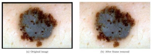
Dermoscopy images often contain black frames that are introduced during the digitization process. These need to be removed because they might interfere with the subsequent lesion localization procedure. In order to determine the darkness of a pixel with (R, G, B) coordinates, the lightness component of the HSL color space [13] is utilized:

$$L=\frac{\max (R,G,B)+\min (R,G,B)}{2}$$ (1)

In particular, a pixel is considered to be black if its lightness value is less than 20. Using this criterion, the image is scanned row-by-row starting from the top. A particular row is labeled as part of the black frame if it contains 60% black pixels. The top-to-bottom scan terminates when a row that contains less than the threshold percentage of pixels is encountered. The same scanning procedure is repeated for the other three main directions. Fig. 1 shows the result of this procedure on a sample image.

Figure 1.

Black frame removal

2.2 Approximate Lesion Localization

Although dermoscopy images can be quite large, the actual lesion often occupies a relatively small area. Therefore, if we can determine the approximate location of the lesion, the border detection algorithm can focus on this region rather than the whole image. An accurate bounding box (the smallest axis-aligned rectangular box that encloses the lesion) might be useful for various reasons: (i) it provides an estimate of the lesion size (certain image segmentation algorithms such as region growing and morphological flooding can use the size of the region as a termination criterion), (ii) it might improve the border detection accuracy since the procedure is focused on a region that is guaranteed to contain the lesion, (iii) it speeds up the border detection since the procedure is performed on a region that is often smaller than the whole image, (iv) its surrounding might be utilized in the estimation of the background skin color, which is useful for various operations including the elimination of spurious regions that are discovered during the border detection procedure [10] and the extraction of dermoscopic features such as blotches [14] and blue-white areas [15].

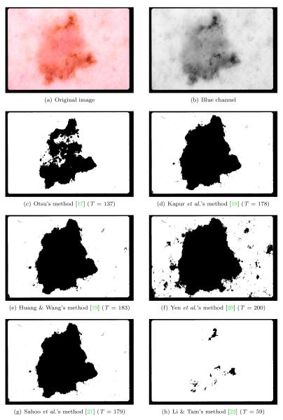
In many dermoscopic images, the lesion can be roughly separated from the background skin using a grayscale thresholding method applied to the blue channel [8][9]. While there are a number of thresholding methods that perform well in general, the effectiveness of a method strongly depends on the statistical characteristics of the image [16]. Fig. 2 illustrates this phenomenon¹. Here, methods 2(d), 2(e), and 2(g) perform quite well. In contrast, methods 2(c) and 2(h) underestimate the optimal threshold, whereas method 2(f) overestimates the optimal threshold. Although method 2(c) is the most popular thresholding algorithm in the literature [23], for this particular image, it performs the second worst.

Figure 2.

Comparison of various thresholding methods (T : threshold)

A possible approach to overcome this problem is to fuse the results provided by an ensemble of thresholding algorithms. In this way, it is possible to exploit the peculiarities of the participating thresholding algorithms synergistically, thus arriving at more robust final decisions than is possible with a single thresholding algorithm. We note that the goal of the fusion is not to outperform the individual thresholding algorithms, but to obtain accuracies comparable to that of the best thresholding algorithm independently of the image characteristics. In this study, we used the threshold fusion method proposed by Melgani [16], which we describe briefly in the following.

Let X = {x_mn : m = 0, 1, … , M — 1, n = 0, 1, … , N — 1} be the original scalar M × N image with L possible gray levels (x_mn ∈ {0, 1, … , L — 1}) and Y = {y_mn : m = 0, 1, … , M — 1, n = 0, 1, … , N — 1} be the binary output of the threshold fusion. Consider an ensemble of P thresholding algorithms. Let T_i and A_i (i = 1, 2, … , P ) be the threshold value and the output binary image associated with the i-th algorithm of the ensemble, respectively. Within a Markov Random Field (MRF) framework the fusion problem can be formulated as an energy minimization task. Accordingly, the local energy function U_mn to be minimized for the pixel (m, n) can be written as follows:

$${\mathrm{U}}_{mn}={\beta }_{SP}\cdot {\mathrm{U}}_{SP}[y_{mn},Y^S(m,n\left)\right]+\sum _{i=1}^P{\beta }_i\cdot {\mathrm{U}}_{II}[y_{mn},A_i^S(m,n\left)\right]$$ (2)

where S is a predefined neighborhood system associated with pixel (m, n), U_SP (·) and U_II(·) refer to the spatial and inter-image energy functions, respectively, whereas β_SP and β_i (i = 1, 2, … , P) represent the spatial and inter-image parameters, respectively. The spatial energy function can be expressed as:

$${\mathrm{U}}_{SP}[y_{mn},Y^S(m,n\left)\right]=-\sum _{y_{pq}\in Y^S(m,n)}\mathrm{I}(y_{mn},y_{pq})$$ (3)

where I(., .) is the indicator function defined as:

$$\mathrm{I}(y_{mn},y_{pq})=\{\begin{array}{cc}1\hfill & \text{if}{y}_{mn}=y_{pq}\hfill \\ 0\hfill & \text{otherwise}\hfill \end{array}\phantom{\}}$$ (4)

The inter-image energy function is defined as:

$${\mathrm{U}}_{II}[y_{mn},A^S(m,n\left)\right]=-\sum _{A_i(p,q)\in A_i^S(m,n)}{\alpha }^i\left(x_{pq}\right)\cdot \mathrm{I}[y_{mn},A_i(p,q\left)\right]$$ (5)

where αⁱ(·) is a weight function given by:

$${\alpha }^i\left(x_{mn}\right)=1-\exp (-\gamma \mid x_{mn}-T_i\mid )$$ (6)

This function controls the effect of unreliable decisions at the pixel level that can be incurred by the thresholding algorithms. At the global (image) level decisions are weighed by the inter-image parameters β_i (i = 1, 2, … , P ), which are computed as follows:

$${\beta }_i=\exp (-\gamma \mid \stackrel{‒}{T}-T_i\mid )$$ (7)

where $\stackrel{‒}{T}$ is the average threshold value:

$$\stackrel{‒}{T}=\frac{1}{P}\sum _{i=1}^P{T}_i$$ (8)

The MRF fusion strategy proposed in [16] is as follows:

1. Apply each thresholding algorithm of the ensemble to the image X to generate the set of thresholded images A_i (i = 1, 2, … , P)

2. Initialize Y by minimizing for each pixel (m, n) the local energy function U_mn defined in Eq. 2 without the spatial energy term i.e., by setting β_SP = 0.

3. Update Y by minimizing for each pixel (m, n) the local energy function U_mn defined in Eq. 2 including the spatial energy term i.e., by setting β_SP ≠ 0.

4. Repeat step 3 K_max times or until the number of different labels in Y computed over the last two iterations becomes very small.

In our preliminary experiments, we observed that, besides being computationally demanding, the iterative part (step 3) of the fusion algorithm makes only marginal contribution to the quality of the results. Therefore, in this study, we considered only the first two steps. The γ parameter was set to the recommended value of 0.1 [16]. For computational reasons, α (Eq. 6) and β (Eq. 7) values were precalculated and the neighborhood system S was chosen as a 3 × 3 square.

The most important performance factor in the fusion algorithm seems to be the choice of the thresholding algorithms. We considered six popular thresholding algorithms to construct the ensemble: Otsu’s [17], Kapur et al.’s [18], Huang & Wang’s [19], Yen et al.’s [20] , Sahoo et al.’s [21], and Li & Tam’s [22] methods. In order to determine the best combination, we evaluated ensembles with 3 (20 ensembles), 4 (15 ensembles), 5 (6 ensembles), and 6 (1 ensembles) methods.

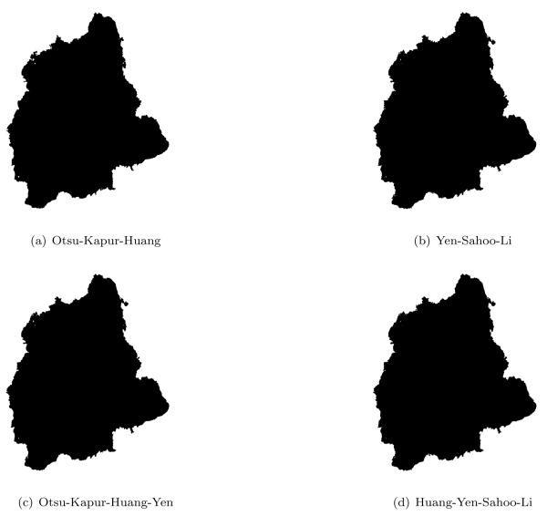
Fig. 3 shows the output of four particular ensembles: Otsu-Kapur-Huang, Yen-Sahoo-Li, Otsu-Kapur-Huang-Yen, and Huang-Yen-Sahoo-Li. Note that each ensemble contains at least one method that either underestimates or overestimates the optimal threshold. It can be seen that each ensemble performs equally well, which demonstrates that failures in pathological cases might be prevented using a proper fusion strategy.

Figure 3.

Comparison of various threshold ensembles

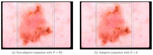
Fig. 4(a) shows the result of the ensemble Otsu-Kapur-Huang-Sahoo. Here, the blue bounding box encloses the dermatologist determined border (see Section 3), whereas the red one encloses the binary output of the threshold fusion. It can be seen that the red box is completely contained within the blue box. This was observed in many cases because the automated thresholding methods tend to find the sharpest pigment change, whereas the dermatologists choose the outmost detectable pigment. We experimented with two different expansion methods to solve this problem. The first one involves expanding the automatic box by P% in four main directions. In other words, an automatic box of size M_B × N_B is expanded by M_B · P/100 pixels in the West and East directions and N_B · P/100 pixels in the North and South directions. The second one involves incrementing the threshold values obtained by each algorithm in the ensemble by G gray levels. In the rest of this article, we will refer to these expansion methods as non-adaptive and adaptive, respectively. Figs. 4(a) and 4(b) show the results of these methods with the expanded box shown in green. In this particular example, the non-adaptive method performs better in bringing the automatic box closer to the manual one. In order to determine the optimal expansion amounts we evaluated P ∈ {2, 4, 6, 8} and G ∈ {4, 6, 8, 10}.

Figure 4.

Comparison of the bounding box expansion methods

3 Results and Discussion

The proposed method was tested on a set of 428 dermoscopy images obtained from the EDRA Interactive Atlas of Dermoscopy [2] and the Keio University Hospital. These were 24-bit RGB color images with dimensions ranging from 771 × 507 pixels to 768 × 512 pixels. An experienced dermatologist (WVS) determined the manual borders by selecting a number of points on the lesion border, which were then connected by a second-order B-spline. The bounding box error was quantified using the grading system developed by Hance et al. [24]

$$\epsilon =\frac{\text{Area}(\text{AutomaticBox}\oplus \text{ManualBox})}{\text{Area}\left(\text{ManualBox}\right)}\cdot 100$$ (9)

where AutomaticBox is the binary image obtained by filling the bounding box of the fusion output, ManualBox is the binary image obtained by filling the bounding box of the dermatologist-determined border, ⊕ is the exclusive-OR operation, which essentially determines the pixels for which the AutomaticBox and ManualBox disagree, and Area(I) denotes the number of pixels in the binary image I.

We determined the optimal parameter combination for the presented approximate bounding box computation method as follows. First, the black frame removal procedure described in Section 2.1 is performed on each image in the data set. The lesion bounding box is then computed using the fusion method described in Section 2.2 with one of the 42 ensembles. Finally, the approximate bounding box is expanded using either the non-adaptive method with P ∈ {2, 4, 6, 8} or the adaptive method with G ∈ {4, 6, 8, 10}. Table 1 shows various statistics associated with the four most accurate ensembles for each expansion method. The last two columns refer to the mean and standard deviation values, respectively for the percentage image size reduction, i.e. $\frac{\text{Area}\left(\text{AutomaticBox}\right)}{M\cdot N}\cdot 100$, provided by the bounding box computation. The following observations are in order: (i) both expansion methods reduce the mean bounding box error, (ii) the lowest mean errors were obtained using the ensemble Otsu-Kapur-Huang-Sahoo, (iii) the non-adaptive expansion method was more effective than the adaptive one, (iv) the computation of the bounding box reduced the original image size by about 260%.

Table 1.

Ensemble statistics (μ: mean, σ: std. dev., ε_i: initial box error, ε_x: expanded box error)

Ensemble	Expansion Method	μ ε i	σ ε i	μ ε x	σ ε x	μ s	σ s
Otsu-Kapur-Huang-Sahoo	Non-adaptive (P = 2)	10.25	8.10	7.58	8.13	268.31	185.64
Otsu-Huang-Yen-Li	Non-adaptive (P = 4)	11.92	7.59	7.89	6.30	260.55	183.85
Otsu-Huang-Sahoo-Li	Non-adaptive (P = 4)	11.98	7.62	7.90	6.20	260.95	184.14
Otsu-Huang-Sahoo	Non-adaptive (P = 2)	11.14	7.17	7.91	6.71	273.84	195.69
Otsu-Kapur-Huang-Sahoo	Adaptive (G = 6)	10.25	8.10	9.27	7.68	276.92	192.14
Kapur-Huang-Sahoo-Li	Adaptive (G = 8)	10.98	7.66	9.43	7.69	279.03	194.42
Otsu-Kapur-Huang-Sahoo	Adaptive (G = 4)	10.25	8.10	9.44	7.56	279.98	194.26
Kapur-Huang-Sahoo-Li	Adaptive (G = 6)	10.98	7.66	9.67	7.58	282.09	196.58

The adaptive method was less effective than the non-adaptive one probably because the former often expands the approximate box by unpredictable amounts: either too little (as in Fig. 4(b)) or too much depending on the shape of the histogram and the value of the G parameter. In contrast, the latter always expands the approximate box by an amount specified by the P parameter.

Table 2 shows the statistics for the individual thresholding methods. Note that, due to space limitations, we report only the results of the non-adaptive expansion method (as in the ensemble case, the adaptive method has inferior performance). It can be seen that, in most configurations, the individual methods obtain significantly higher mean errors than the best ensemble methods, i.e. the first four rows of Table 1. This is because, as explained in Section 2.2, the individual methods are more prone to catastrophic failures when given pathological input images. The high standard deviation values also support this explanation. Only the performance of Otsu (with P = 2, 4) and Li et al.’s (with P = 4) methods is close to the performance of the ensembles. However, as mentioned in Section 2.2, the goal of fusion is not to outperform the individual thresholding algorithms, but to obtain accuracies comparable to that of the best thresholding algorithm independently of the image characteristics.

Table 2.

Individual statistics (μ: mean, σ: std. dev., ε_i: initial box error, ε_x: expanded box error)

Thresholding Method	Expansion Method	μ ε i	σ ε i	μ ε x	σ ε x	μ s	σ s
Otsu	Non-adaptive (P = 2)	12.05	9.10	9.00	8.95	275.07	199.28
Kapur	Non-adaptive (P = 2)	12.87	16.86	12.68	17.56	261.95	197.94
Huang	Non-adaptive (P = 2)	20.31	67.97	17.17	69.76	269.59	190.09
Yen	Non-adaptive (P = 2)	14.98	27.12	15.74	27.74	255.61	250.53
Sahoo	Non-adaptive (P = 2)	13.43	24.60	13.37	25.19	254.43	184.36
Li	Non-adaptive (P = 2)	15.12	9.65	11.06	9.07	293.54	215.80
Otsu	Non-adaptive (P = 4)	12.05	9.10	9.10	9.14	256.86	182.82
Kapur	Non-adaptive (P = 4)	12.87	16.86	15.54	18.61	245.36	183.78
Huang	Non-adaptive (P = 4)	20.31	67.97	16.83	70.69	251.99	174.44
Yen	Non-adaptive (P = 4)	14.98	27.12	19.32	28.49	239.46	230.91
Sahoo	Non-adaptive (P = 4)	13.43	24.60	16.43	25.98	238.32	170.38
Li	Non-adaptive (P = 4)	15.12	9.65	9.41	7.99	273.93	198.61

As mentioned in Section 2.2, an accurate bounding box can provide an estimate of the lesion size, i.e. Area(ManualBorder). In order to verify this, we calculated the best fitting line for Area(AutomaticBox ) vs. Area(ManualBorder) using the generalized least-squares method [25]:

$$\text{Area}\left(\text{ManualBorder}\right)\approx \text{Area}\left(\text{AutomaticBox}\right)\cdot 0.861271-15627.226419$$ (10)

where ManualBorder is the binary image obtained by filling the dermatologist-determined border. The accuracy of this relation was calculated by plugging the area of the approximate bounding box for each image into Eq. 10, and then comparing the result with the actual area of the lesion, which is calculated from the dermatologist-determined border. The percentage mean and standard deviation errors over the entire image set were 11.88 and 11.49, respectively. These results demonstrate that the lesion size can be estimated from the bounding box area with relatively high accuracy. An even better estimate can be made from the binary output of the threshold fusion. The best fitting line for Area(FusionOutput) vs. Area(ManualBorder) was calculated as:

$$\text{Area}\left(\text{ManualBorder}\right)\approx \text{Area}\left(\text{FusionOutput}\right)\cdot 1.158209-4485.287871$$ (11)

where FusionOutput is the binary output of the threshold fusion. The percentage mean and standard deviation errors for this relation were 8.16 and 8.54, respectively.

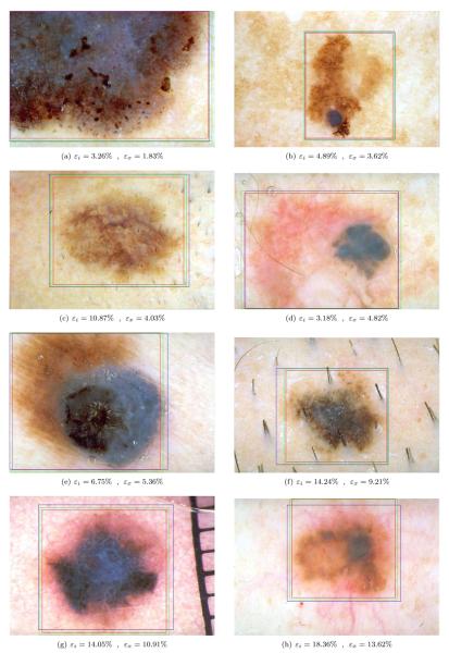
Fig. 5 shows sample bounding box computation results obtained using the ensemble Otsu-Kapur-Huang-Sahoo with P = 2. It can be seen that the presented method determines an accurate bounding box even for lesions with fuzzy borders. We note that while the expansion operation is useful in most cases, in some cases such as Fig. 5(d), it might deteriorate the results slightly.

Figure 5.

Sample bounding box computation results (ε_i: initial box error, ε_x: expanded box error)

4 Conclusions

In this paper, an automated method for approximate lesion localization in dermoscopy images is presented. The method is comprised of three main phases: black frame removal, initial bounding box computation using an ensemble of thresholding algorithms, and expansion of the initial bounding box. The execution time of the method is about 0.15 seconds for a typical image of size 768 × 512 pixels on an Intel Pentium D 2.66Ghz computer.

The presented method may not perform well on images with significant amount of hair or bubbles since these elements alter the histogram, which in turn results in biased threshold computations. For images with hair, a preprocessor such as DullRazor™ [11] might be helpful. Unfortunately, the development of a reliable bubble removal method remains an open problem.

Future work will be directed towards testing the utility of the presented method in a border detection study. The implementation of the threshold fusion method will be made publicly available as part of the Fourier image processing and analysis library, which can be downloaded from http://sourceforge.net/projects/fourier-ipal

References

- [1].Jemal A, Siegel R, Ward E, et al. Cancer Statistics, 2008. CA: A Cancer Journal for Clinicians. 2008;58(2):71–96. doi: 10.3322/CA.2007.0010. 2008. [DOI] [PubMed] [Google Scholar]
- [2].Argenziano G, Soyer HP, De Giorgi V, et al. Dermoscopy: A Tutorial. EDRA Medical Publishing & New Media; Milan, Italy: 2002. [Google Scholar]
- [3].Steiner K, Binder M, Schemper M, et al. Statistical Evaluation of Epiluminescence Dermoscopy Criteria for Melanocytic Pigmented Lesions. Journal of American Academy of Dermatology. 1993;29(4):581–588. doi: 10.1016/0190-9622(93)70225-i. [DOI] [PubMed] [Google Scholar]
- [4].Binder M, Schwarz M, Winkler A, et al. Epiluminescence Microscopy. A Useful Tool for the Diagnosis of Pigmented Skin Lesions for Formally Trained Dermatologists. Archives of Dermatology. 1995;131(3):286–291. doi: 10.1001/archderm.131.3.286. [DOI] [PubMed] [Google Scholar]
- [5].Fleming MG, Steger C, Zhang J, et al. Techniques for a Structural Analysis of Dermatoscopic Imagery. Computerized Medical Imaging and Graphics. 1998;22(5):375–389. doi: 10.1016/s0895-6111(98)00048-2. [DOI] [PubMed] [Google Scholar]
- [6].Schmid P. Segmentation of Digitized Dermatoscopic Images by Two-Dimensional Color Clustering. IEEE Trans. on Medical Imaging. 1999;18(2):164–171. doi: 10.1109/42.759124. [DOI] [PubMed] [Google Scholar]
- [7].Erkol B, Moss RH, Stanley RJ, Stoecker WV, Hvatum E. Automatic Lesion Boundary Detection in Dermoscopy Images Using Gradient Vector Flow Snakes. Skin Research and Technology. 2005;11(1):17–26. doi: 10.1111/j.1600-0846.2005.00092.x. [DOI] [PMC free article] [PubMed] [Google Scholar]
- [8].Iyatomi H, Oka H, Saito M, et al. Quantitative Assessment of Tumor Extraction from Dermoscopy Images and Evaluation of Computer-based Extraction Methods for Automatic Melanoma Diagnostic System. Melanoma Research. 2006;16(2):183–190. doi: 10.1097/01.cmr.0000215041.76553.58. [DOI] [PubMed] [Google Scholar]
- [9].Celebi ME, Aslandogan YA, Stoecker WV, et al. Unsupervised Border Detection in Dermoscopy Images. Skin Research and Technology. 2007;13(4):454–462. doi: 10.1111/j.1600-0846.2007.00251.x. [DOI] [PMC free article] [PubMed] [Google Scholar]
- [10].Celebi ME, Kingravi HA, Iyatomi H, et al. Border Detection in Dermoscopy Images Using Statistical Region Merging. Skin Research and Technology. doi: 10.1111/j.1600-0846.2008.00301.x. (in press) [DOI] [PMC free article] [PubMed] [Google Scholar]
- [11].Lee TK, Ng V, Gallagher R, et al. Dullrazor: A Software Approach to Hair Removal from Images. Computer in Biology and Medicine. 1997;27(6):533–543. doi: 10.1016/s0010-4825(97)00020-6. [DOI] [PubMed] [Google Scholar]
- [12].Zhou H, Chen M, Gass R, et al. Feature-Preserving Artifact Removal from Dermoscopy Images. Proc. of the SPIE Medical Imaging 2008 Conf. 6914:1B1–9. [Google Scholar]
- [13].Levkowitz H, Herman GT. GLHS: A Generalized Lightness, Hue, and Saturation Color Model. CVGIP: Graphical Models and Image Processing. 1993;55(4):271–285. [Google Scholar]
- [14].Stoecker WV, Gupta K, Stanley RJ, et al. Detection of Asymmetric Blotches in Dermoscopy Images of Malignant Melanoma Using Relative Color. Skin Research and Technology. 2005;11(3):179–184. doi: 10.1111/j.1600-0846.2005.00117.x. [DOI] [PMC free article] [PubMed] [Google Scholar]
- [15].Celebi ME, Kingravi HA, Aslandogan YA, Stoecker WV. Detection of Blue-White Veil Areas in Dermoscopy Images Using Machine Learning Techniques. Proc. of the SPIE Medical Imaging 2006 Conf. 6144:1861–1868. [Google Scholar]
- [16].Melgani F. Robust Image Binarization with Ensembles of Thresholding Algorithms. Journal of Electronic Imaging. 2006;15(2):023010. (11 pages) [Google Scholar]
- [17].Otsu N. A Threshold Selection Method from Gray Level Histograms. IEEE Trans. on Systems, Man and Cybernetics. 1979;9(1):62–66. [Google Scholar]
- [18].Kapur JN, Sahoo PK, Wong AKC. A New Method for Gray-Level Picture Thresholding Using the Entropy of the Histogram. Graphical Models and Image Processing. 1985;29(3):273–285. [Google Scholar]
- [19].Huang L-K, Wang M-JJ. Image Thresholding by Minimizing the Measures of Fuzziness. Pattern Recognition. 1995;28(1):41–51. [Google Scholar]
- [20].Yen JC, Chang FJ, Chang S. A New Criterion for Automatic Multilevel Thresholding. IEEE Trans. on Image Processing. 1995;4(3):370–378. doi: 10.1109/83.366472. [DOI] [PubMed] [Google Scholar]
- [21].Sahoo PK, Wilkins C, Yeager J. Threshold Selection Using Renyi’s Entropy. Pattern Recognition. 1997;30(1):71–84. [Google Scholar]
- [22].Li CH, Tam PKS. An Iterative Algorithm for Minimum Cross Entropy Thresholding. Pattern Recognition Letters. 1998;18(8):771–776. [Google Scholar]
- [23].Sezgin M, Sankur B. Survey over Image Thresholding Techniques and Quantitative Performance Evaluation. Journal of Electronic Imaging. 2004;13(1):146–165. [Google Scholar]
- [24].Hance GA, Umbaugh SE, Moss RH, Stoecker WV. Unsupervised Color Image Segmentation with Application to Skin Tumor Borders. IEEE Engineering in Medicine and Biology. 1996;15(1):104–111. [Google Scholar]
- [25].Li HC. A Generalized Problem of Least Squares. American Mathematical Monthly. 1984;91(2):135–137. [Google Scholar]