TT2NE: a novel algorithm to predict RNA secondary structures with pseudoknots

Abstract

We present TT2NE, a new algorithm to predict RNA secondary structures with pseudoknots. The method is based on a classification of RNA structures according to their topological genus. TT2NE is guaranteed to find the minimum free energy structure regardless of pseudoknot topology. This unique proficiency is obtained at the expense of the maximum length of sequences that can be treated, but comparison with state-of-the-art algorithms shows that TT2NE significantly improves the quality of predictions. Analysis of TT2NE's incorrect predictions sheds light on the need to study how sterical constraints limit the range of pseudoknotted structures that can be formed from a given sequence. An implementation of TT2NE on a public server can be found at http://ipht.cea.fr/rna/tt2ne.php.

INTRODUCTION

In the past 20 years, there has been a tremendous increase of interest in RNA by the biological community. This biopolymer, which was at first merely considered as a simple information carrier, was gradually proven to be a major actor in the biology of the cell (1). It was first discovered that some RNAs have enzymatic activity (ribozymes) and as such would directly play a crucial role in the biochemical reactions taking place in the cell. More recently, it was also discovered that some RNAs, in particular micro-RNAs, have a post-transcriptional regulation role in the cell by controlling the level of translation of some messenger RNAs: more than 60% of human protein-coding genes have been under selective pressure to maintain pairing to micro-RNAs (2). At present, it is also believed that a considerable amount of ‘junk’ (non-coding) DNA is transcribed into some non-coding RNAs, the role of which is still unclear.

Since the RNA functionality is mostly determined by its 3D conformation, the accurate prediction of RNA folding from the nucleotide sequence is a central issue (3). It is strongly believed that the biological activity of RNA (be it enzymatic or regulatory), is implemented through the binding of some unpaired bases of the RNA with their ligand. It is thus crucial to have a precise and reliable map of all the pairings taking place in RNA and to correctly identify loops. The complete list of all Watson–Crick and Wobble base pairs in RNA is called the ‘secondary structure’ of RNA.

Since the folding of even short RNA molecules takes too long to perform with all-atom molecular dynamics simulations including explicit solvent, the more modest goal of solely obtaining the most probable secondary structures based on experimentally derived base-pairing and base-stacking free energies has been pursued. There is convincing evidence showing that, as in NMR protein structure prediction, the secondary structure of RNAs is sufficiently constraining to entirely and unambiguously determine the 3D structure of the molecule (4). This 3D structure of the RNA in turn controls the biochemistry of the molecule, by making certain regions of its surface accessible to the ligand molecule.

In this article, we will adhere to the notion that there is an effective free energy which governs the formation of secondary structures, so that the optimal folding of an RNA sequence is found as the minimum free energy structure (MFE for short). The problem of finding the MFE structure given a certain sequence has been conceptually solved provided the MFE is planar, i.e. the MFE structure contains no pair (i, j), (k, l) such that i < k < j < l. In that case, polynomial algorithms which can treat long RNAs assuming a mostly linear free energy model have been found (5–7). Otherwise, the MFE structure is said to contain pseudoknots and finding it has been shown to be an NP-complete problem with respect to the sequence length (8). Even if pseudoknots represent a small part of known structures, they often have a functional role (9,10) and the problem of their prediction must be addressed.

Three main algorithmic strategies can be thought of to take into account the NP-completeness of pseudoknotted MFE prediction: (i) empirical search of the MFE using heuristic methods (11–14), (ii) efficient exact calculations on a restricted class of pseudoknots (15–17) and (iii) exact calculations, using various tricks to allow for the treatment of sequences as large as possible (18).

Here we present TT2NE, an algorithm that falls into the latter category. TT2NE relies on the ‘maximum weighted independent set’ (WIS) formalism. In this formalism, an RNA structure is viewed as an aggregate of stem-like structures (helices possibly comprising bulges of size 1 or internal loops of size 1 × 1). These stem-like structures can be viewed as points in the space of all helical fragments available from a given sequence and we will refer to them as ‘helipoints’. Please note that our notion of helipoints is in fact not trivial and differs from what is done in algorithms based on the WIS formalism, where they generally reduce to maximum helices (see the explanation in ‘Material and Methods’ Section). Given a certain sequence, the set of all possible helipoints is computed and a weighted graph is built. The vertices of the graph are the helipoints, with a weight given by −1 times their free energy of formation. Two vertices are connected by an arc if and only if the corresponding helipoints are not compatible in the same secondary structure. Indeed, two helipoints may be mutually exclusive in a graph: this is for example the case if they share at least one base (since base triples are forbidden). Finding the MFE structure thus amounts to finding the maximum weighted independent set of the graph, i.e. the set of pairwise compatible helipoints such that the overall free energy is minimum.

Given a certain sequence x, let's denote N_x the number of available helipoints and the associated graph. The core routine of TT2NE is a simple exhaustive depth exploration of all independent sets of using a backtracking procedure, where vertices are added to the current structure in the increasing order of their free energy, that is decreasing order of weight (see black pseudocode in Figure 1). There is in particular no restriction on the pseudoknots topologies that TT2NE can generate. However, this strategy is very inefficient. In this article we propose two ideas to improve it. First, we use a new treatment of pseudoknots that restrict TT2NE's search to a much smaller and relevant subspace of independent sets. Secondly, we take advantage of a peculiar energy model to enforce a branch-and-bound procedure that speeds up the search of the MFE without loss of exactness. A server implementation of TT2NE can be found at http://ipht.cea.fr/rna/tt2ne.php

Figure 1.

Pseudocode of TT2NE. The core routine is written in black and performs an exhaustive enumeration of all independent sets of . In the end, the MFE structure can be read in the global variable ΔF_cm. The two red lines are improvements discussed in the text.

A new treatment of pseudoknots

In a previous series of studies (19,20), we have proposed a classification of pseudoknots according to their topological genus. The genus is an integer number that captures the complexity of a pseudoknot. Consider the graph of the pairings of an RNA. We first close the extremities of the backbone of the RNA to make a circle, leaving the pairings outside the circle. Some of the pairings may cross each other. The genus of the RNA graph is defined as the number of handles one has to carve in a sphere to be able to draw the RNA graph without any crossing. For instance, all graphs without crossings [i.e. those summed by the algorithm of McCaskill (7)] can be drawn on a sphere; thus they are of genus 0. The standard H-pseudoknot cannot be drawn without crossing on a sphere, but can be on a torus (20). It is thus of genus 1. In addition, the genus is an additive quantity: if there are several pseudoknots in an RNA, the total genus of the RNA is the sum of the genii of its pseudoknots.

We have shown that naturally occurring pseudoknots have a much lower genus than expected in randomly paired polymers (20). In particular, we have shown that for sequences of sizes up to 500 nt, RNA structures may comprise several pseudoknots with individual genii smaller than 2. For sizes around 1500 nt, the genus ranges between 2 and 6. Finally, for the largest RNAs (around 3000 nt) the total genus may reach 17.

We use this fact to guide TT2NE's search of relevant pseudoknots in two ways. First, a penalty for pseudoknot formation depending on their genus is introduced in the free energy model. Although more sophisticated forms could be imagined, for now we chose a simple linear form, dictated by the fact that as we mentioned before, the genus is additive. A pseudoknot of genus g is assigned a penalty +μg where we set μ to +1.5 kcal/mol. This value of μ was obtained by optimizing the number of correctly predicted base pairs by our algorithm. Second, an upper limit g_max is introduced. This limit, tunable by the user, has a critical importance as it defines the space of pseudoknots where TT2NE will restrict its search. The size of this space grows exponentially with g_max (21), so this number has a great impact on the computational time required by TT2NE. Based on the relation of RNA size to genus mentioned above, we may safely fix a maximum genus of 3 for RNA sizes smaller than 250, typically the maximal size we can treat with our present algorithm due to computational time constraints.

We have shown that the most standard pseudoknots, i.e. the H-pseudoknot (ABAB topology) and the kissing-hairpins (ABACBC topology), have both genus 1. It implies that if one is interested in short chains which carry these kind of pseudoknots, setting g_max to 1 is sufficient and would save a lot of computational time. Setting g_max to a large value would leave the problem as open as possible, but again, a wise tuning of this parameter proves to be a relevant and efficient way to locate the MFE in a fast way.

A branch-and-bound procedure

The core routine of TT2NE can be improved using a branch-and-bound procedure. The idea is to speed up the search of the MFE of by computing first the MFE of some relevant subgraphs. The crux of such a branch-and-bound procedure is to be able to relate those partial solutions to the general problem and this can be done in TT2NE by taking advantage of a peculiar energy model.

Energy model

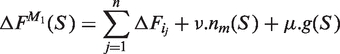
Vertices are sorted in increasing order of free energy, i.e. the vertex 1 represents the most favorable helipoint. We denote ΔF_p the free energy of the p-th vertex (the way to compute the free energy of a helipoint is defined in the next subsection, in Equation 4). Then in TT2NE the free energy of a structure S made of n helipoints {h_i1, h_i2, … , h_in} is computed with the following model M₁:

(1)

where n_m(S) is the number of multi-branch loops of S and ν is the corresponding penalty of formation. Note that in this model there is no term for large internal loops or bulges, nor a penalty depending on the number of branches of multi-branch loops. In our present implementation of TT2NE, we did not include any penalty for multi-branch loops formation, i.e. we set ν = 0.

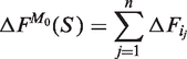
We also introduce the simple model M₀ where the free energy of S is just the sum of the free energies of the helipoints it is made of:

(2)

Property

Let ΔF_min(i) be the MFE of structures comprised of helipoints with indices larger than i, according to the energy model M₀. ΔF_min(i) would simply be the output of TT2NE when used on the restriction of to its N_x − i last vertices with model M₀. Let S⁰ be a structure made of n helipoints and i_n the index of its least stable helipoint. Let's denote r^k(S) the restriction of a structure S to its k most stable helipoints. Then it can be straightforwardly shown that the following property holds:

(3)

The practical meaning of this relation is: there is a lower limit to the free energy of all structures that can be derived from S⁰ by adding any combination of helipoints of indices larger than i_n. Consequently, if this lower limit is found to be larger than the current MFE that TT2NE has found so far, TT2NE can safely ignore all these structures: the global MFE cannot be found in this ensemble. This property thus allows to further restrict the size of the search space for the MFE.

Those two improvements can be incorporated in TT2NE as can be seen in red in Figure 1.

MATERIALS AND METHODS

Generation of the initial graph

We define a helix as a stack of base pairs possibly comprising bulges of size 1 or internal loops of size 1 × 1. A helipoint is an ensemble of helices that are demarcated by the same extremal (initial and terminal) base pairs. They are closely related to the 4-index matrix Δ_ij,kl introduced in (19,22), where they are defined as the sum of all ladder diagrams (diagrams with no crossing pairing lines in between) between extremal pairs, and satisfy a simple recursion equation. Given two extremal pairs (i, j ) and (k, l ), the set of all helices that end with these two pairs can be generated and their individual energies calculated according to a given energy model. 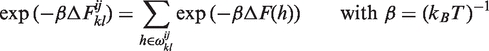The free energy of the helipoint is then computed as

(4)

where ΔF(h) is the free energy of formation of helix h.

In our implementation, when computing this sum, helices of non-negative (i.e. unfavorable) energies are neglected, since their Boltzmann weight would strongly suppress their contribution. Helipoints are stem-like structural building blocks which account for all possible internal pairing possibilities that occur between their extremal pairs. The importance of this notion is well captured by considering for example such a sequence: GGGAGGG […] CCCUUCCC. As one can see, a helix containing a ‘bulged’ uracil can be formed from this sequence, but there are two ways to choose the ‘bulged’ uracil. In order to describe this fact appropriately in statistical mechanics, it is important not to neglect any of these possibilities nor to consider them as distinct competitors. Rather, the notion of helipoint implies that both possibilities would ‘stabilize’ the pairing of these regions of the sequence. In this example, the calculation of the free energy according to Equation 4 would indeed introduce an entropic bonus of −k_BTln2 that accounts for this variability.

The computation of the free energy of all helipoints requires the setting of some values for the basic structural elements of RNA folds: stacking, terminal mismatches, helix formation penalty, bulges and internal loops. The three first families of terms have been taken from Mathews et al. (23). We computed the free energy of the bulges of size one as the energy of the stack of pairs closing this bulge plus 3.8 kcal/mol. The energy of a helix comprising a 1 × 1 internal loop is computed as the sum of the free energies of the two helices delimited by this internal loop minus 3.85 kcal/mol. Larger internal loops and bulges of size more than one were not taken into account. In particular, helipoints do not include such kind of motifs. The multibranch loop formation penalty was not used (i.e. set to 0) in the work presented here, even though TT2NE could handle it. Only helipoints of favorable (i.e. negative) free energies were kept to build the graph. Note that in most other algorithms based on the WIS formalism, only ‘maximal’ favorable helices are kept (i.e. helices such that the outer nearest neighbors of their extremal pairs cannot pair). Our choice not to restrict our algorithm to maximal helipoints makes the problem harder since it makes the graph wider, but the reason will be explained in the discussion part below.

Two helipoints are considered incompatible (i.e. they are connected in the graph) if they overlap, if their concatenation generates an existing helipoint or if their concatenation produces a sterically impossible structure.

This last requirement anticipates a point that will be explained in the ‘Comments and discussion’ section.

Efficient calculation of the genus

TT2NE requires to be able to efficiently update the genus of a structure upon addition or removal of a helipoint. In order to do so, we use a technique which was introduced by t'Hooft (24). A structure of RNA is represented as a diagram whose arcs are double lines that connect paired bases (see Figure 2).

Figure 2.

Examples of how to calculate the genus with a double-line diagram representation. (a) P=5, L=5 → g=0, (b) P=5, L=3 → g=1.

In this process, loops are created within those diagrams and it can be shown that the genus g of the corresponding structures can simply be calculated with:

(5)

where P is the number of pairs and L the number of loops. Upon addition of a new pair to a structure, the genus variation Δg is given by

(6)

We found a property that allows to calculate the term ΔL in an efficient way (the idea of the proof is given as supplementary information). Upon addition of a pair (i, j) to a certain diagram,

(7)

Therefore, Δg can be straightforwardly calculated by checking whether the newly paired bases belong to the same loop and this operation can be efficiently performed in a time linear in the number of pairs of the diagram. The case of the removal of a pair is symmetric.

Branch-and-bound procedure

The Equation 4 requires a prior computation of the terms ΔF_min(i), that is the MFE of restricted to helipoints of index larger than i. Those quantities are obtained by running TT2NE on those subgraphs. However, calculating those terms for all i is useless since the only needed quantity is ΔF_min(1). Rather, one must choose a certain level up to which these terms should be calculated, in order to get a good balance between the time spent in doing so and the time saved later in the search of the MFE. In the work presented here, we generally computed the quantities ΔF_min(i) for the 300 least stable helipoints.

Suboptimal structures

The algorithm presented here only outputs the MFE. It is very easy to adapt it to output a certain number (specified by the user) of suboptimal structures, if needed. This option is available on TT2NE's web server at http://ipht.cea.fr/rna/tt2ne.php.

Heuristic

For longer sequences, a heuristic can be used: the above techniques are first applied to the restriction of the graph to its N_h most stable helipoints and the best structures output are then saturated with the remaining helipoints. This heuristic is identical to the initial problem with N_h = N_x and becomes less and less precise as N_h/N_x → 0.

DETAILED RESULTS

We compared TT2NE with McQfold (12), HotKnots (13), ProbKnots (14) and Mfold (25) on a set of 47 sequences. The sequences that were chosen are a subset of those used in the HotKnots paper (13), supplemented by a set of experimentally determined structures. We have avoided using too many structures inferred by sequence comparison, as its output is not reliable.

The results are displayed as a Supplementary Data (‘Results.pdf’). This set includes most of the sequences on which HotKnots has been tested and shown to perform better than ILM and PKnots-rg, so we will not compare TT2NE to these latter algorithms. We did not compare TT2NE with the Pknots algorithm of Rivas and Eddy (26) as its computation time is very long (it scales like the 6th power of the length of the sequence).

Most of the native structures of genus 1 have the topology of the H-pseudoknot except for sequences 1u8d, CoxB3, HCV_229E, satRPV which are kissing-hairpins and Ec_alpha which is the only known example of the ABCABC topology. Structures of higher genus are generally concatenation of H-pseudoknots except for HDV which has a more complex topology and PSIV_IRES which contains an H-pseudoknot ‘nested’ into another one.

For each sequence, sensitivity and positive predicted value (PPV) have been measured. The sensitivity is defined as the fraction of correctly predicted pairs of the native structure. The PPV is defined as the fraction of correctly predicted pairs of the predicted structure. In all those tests, TT2NE's parameter g_max was set to 3 and μ to 1.5 kcal/mol. This value of μ was obtained by optimization on this very set of sequences but this setting will be discussed below. The sequences, the native structures and TT2NE's predictions are given in detail as Supplementary Data (‘Detailed-structures.txt’)

The total number of base pairs to be predicted in this set is 1115. Mfold, HotKnots, McQfold, ProbKnots and TT2NE, respectively predicted 618, 671, 740, 669 and 870 of them. The total number of base pairs predicted is respectively 1024, 1019, 991, 1041 and 1146. On the average, TT2NE achieves better performance on this set. The statistical significance of this better performance of TT2NE is supported by a t-test analysis. In terms of sensitivity, comparing TT2NE with ProbKnots, McQfold, HotKnots and Mfold, respectively yields a t-value of 4.6, 1.8, 2.5, 5.1. Given the size of our samples (N = 47), this corresponds to a P-value smaller than 0.05 (except for McQfold, for which P ≈ 0.08). Therefore, as far as the sensitivity is concerned, TT2NE outperforms the other algorithms. For the PPV, we find t-values of 4.6, 0.2, 1.7 and 3.3. This shows that TT2NE significantly outperforms Mfold, HotKnots and ProbKnots, but not McQfold. The size of our sample is thus sufficiently large to satisfactorily discriminate between TT2NE and the other algorithms, except for McQfold in terms of the PPV. One might wonder whether this statistical similarity of McQfold and TT2NE implies the similarity of the predicted MFEs. To answer this question, we computed the correlation between the two sets of predicted MFEs, defined as the ratio of the pairs common to both MFEs and the average number of pairs of the two MFEs. This correlation is equal to 1 if the MFEs are identical and 0 if they have no common pair. We found a correlation of 62%, smaller than the average sensitivities and PPVs of both methods. This is a good evidence that the two algorithms predict MFEs which are different in nature. It is thus judicious to use both methods to predict pseudoknots.

Comparison between TT2NE and HotKnots shows that the novelties of TT2NE, namely finding the MFE and introducing a genus penalty, are responsible for the improvement in the quality of the predictions, since HotKnots and TT2NE use essentially the same energy model. ProbKnot achieves approximately the same average results as HotKnots, but it fails to predict even one single structure correctly on this set of mostly experimental structures. Moreover, ProbKnots predicts pseudoknotted structures for only 3 out of 47 sequences. In terms of sensitivity, HotKnots and ProbKnots improve by 6% on average on Mfold, which predicts only pseudoknot-free sequences.

McQFold is the second best algorithm on this set of sequences and could certainly be further improved, as it uses a minimalist energy model and does not include the constraint that a hairpin loop should be at least 3 bases long. Trying to elucidate the success rates of these different algorithms, we have calculated how each algorithm's predictions correlates with Mfold's, i.e. we calculated what fraction of each MFE belongs to Mfold's MFE. As Mfold achieves a sensitivity of 55% on this set of sequences, an ideal algorithm should have a correlation of 55% with Mfold (note that the inverse is not true). We found that TT2NE has 56% correlation, McQfold 65%, HotKnots 74% and ProbKnots 78%. HotKnots and ProbKnots both rely partly on Mfold: both build their prediction on the basis of the calculation of likeliness of base pairs (ProbKnots) or ‘hotspots’ (HotKnots) in a pseudoknot-free context. It is therefore not a surprise to see a higher correlation between HotKnots, ProbKnots and Mfold than between McQfold, TT2NE and Mfold. The fact that Mfold only achieves a sensitivity 55% shows that the problem of pseudoknot prediction is not a simple ‘extension’ of the problem of prediction of pseudknot-free structures, in the sense that in most cases the pseudoknotted MFE is not the pseudoknot-free MFE in which some helices have been added. On the average, half of the structures predicted by Mfold must be folded differently, but which half? We think this is the reason why heuristics based on Mfold (or Mc Caskill's recursion relations) have poorer performance than TT2NE which does find the MFE.

Comments and discussion

Despite the fact that TT2NE can find any type of topology and guarantees to output the MFE, it does not achieve a 100% success. Why is that so? We have investigated the errors generated by TT2NE and we see that they fall in two categories: the first relates to the limit of the energy model used and the second is more specific to the nature of pseudoknots. Of course, in the case of structures proposed through sequence comparison, one cannot rule out the possibility that those speculated structures are actually wrong.

Limits due to the free energy model

The Turner free energy model has been shown to be partly unable to explain planar secondary structures (27). TT2NE uses only a subset of this model: thus, there are errors coming from the part of this model we use, and others coming from the part we do not use.

An example of the first case is provided by the sequence satRPV: the native secondary structure is almost correctly predicted, but an error is made because the helix is considered more thermodynamically favorable than the native one . An other example can be seen with the sequence TEV: the computed energy of its short helices is found to be not favorable enough to form a pseudoknot.

An example of errors due to the inability of TT2NE of correctly computing the energy of long internal loops can be seen with Ec-RpmI. There, the native structure contains a helipoint containing a 2 × 1 internal loop. The thermodynamics properties of 2 × 1 internal loops are not properly taken into account in TT2NE. As a consequence, the energy of formation of that helipoint is not found to be negative and therefore it is not recognized as a relevant helipoint to store into the initial graph. In other words, this helipoint is not favorable and is thus not kept in the construction of the graph. This problem could be solved by allowing for the inclusion of 2 × 1 internal loops but this would dramatically increase the number of possible helipoints and the running time of TT2NE would grow exponentially.

Limits due to the absence of steric constraints

We also realized that predicting a pseudoknot is not only a question of free energy minimization: steric constraints also matter and some predicted sets of helipoints must sometimes be rejected because they do not correspond to any feasible geometry in 3D space. For example, here is a feature observed in the second best secondary structure predicted for the sequence Ec_alpha (using a parsing representation):

This pseudoknot is made of two helices respectively drawn in blue and black. Let's focus on the seven bases of the 5′ strand of the black helix (ACGGGCU). The geometry of the nucleotides implies that the pairings organize according to the canonical A-helix shape. However, those seven bases also connect the two ends of the blue helix: they should therefore make up a hairpin loop. It is clear that these two kinds of geometry are mutually exclusive. This diagram therefore cannot match a real RNA structure and must be rejected. To create a sterically allowable pseudoknot between those regions, one or both helices should be shortened. We thus think that a perfect pseudoknot prediction algorithm should be able to include non-maximal helices. This necessity is also very well illustrated by the example of the mouse mammary tumor virus pseudoknot whose 3D structure has been resolved (PDB entry: 1rnk) (28). This pseudoknot is an H-pseudoknot and one of its helices is non-maximal. By looking at the sequence, one could think that one additional Wobble pair could form but from looking at the 3D structure, it is clear that due to the peculiar geometry of this pseudoknot, the bases of the putative pair are in fact too far from each other to be able to pair. All algorithms tested on that sequence wrongly predict this additional pair (sensitivity of 1 but PPV of 0.91). We thus have chosen by design to include all possible favorable non-maximal helipoints in the initial graph that TT2NE generates, even though it makes calculations longer.

In fact, it is worth noticing that whenever a pseudoknot is predicted by TT2NE, its PPV is almost always less than (or equal to) the sensitivity. This means that the predicted structures are somewhat overloaded with spurious pairings. We examined TT2NE's predicted MFEs and we are convinced that most of the time, the helipoints predicted in excess cannot exist due to steric considerations. This point therefore raises an important difference in the evaluation of algorithms for the prediction of secondary structures with and without pseudoknots, such as Mfold. For the latter, if some modifications entail an overall improvement of the sensitivity and the PPV of the predicted MFEs, then we can conclude that the predictive power of such an algorithm has been improved. In contrast, with pseudoknot prediction algorithms, such an improvement can be misleading. In fact, the real output to be taken into account is not the MFE but the first sterically possible structure. Even if the predicted MFE has good sensitivity and PPV, it may happen that the best sterically possible structure is in fact completely different and has a bad score. For example, TT2NE's prediction for the sequence GLV_IRES has a sensitivity of 100% but a PPV of 85%: it contains an additional helix that may render the structure sterically impossible. Would the sensitivity and the PPV of the first sterically possible structure be as good? We therefore think that the problem of the determination of sterically impossible structures is essential. As long as we do not know how to detect impossible structures in a fast and efficient way, pseudoknot prediction algorithms may output lots of impossible structures and the evaluation of such algorithms with standard statistical estimates such as sensitivity and PPV of the MFE may be meaningless. How to deal properly with steric constraints? To our knowledge this is an open question. No clear criteria is known to decide whether a proposed pseudoknot is possible or not. It would be an easy task though to include such a criteria in TT2NE as far as only two helipoints are involved (that is the case of simple H-pseudoknots). Indeed, during the generation of the initial graph, it is sufficient to declare two helipoints incompatible if they form a sterically impossible pseudoknot. In this version of TT2NE, we have used a simple test depicted in Figure 3. However, this test is not foolproof as TT2NE still wrongly predicts the Wobble pair in the case discussed above.

Figure 3.

Naive stericity tests used in this work for H-pseudoknots. The constraint (*) is used to prevent the formation of real knots.

Topological control

TT2NE allows to partly overcome the two main aforementioned problems through parameters μ and g_max. Indeed, the user can play on these parameters to scan the space of possible pseudoknots in order to get other good candidates with a genus different from the MFE predicted by TT2NE. In five cases, TT2NE predicted structures of higher genus than the native one and a proper 3D-modeling would certainly show that each of these structures must be rejected due to steric constraints. TT2NE offers the possibility to limit the complexity of the predicted pseudoknot by playing with the parameter g_max. We therefore folded again these five sequences with an appropriate setting of g_max, which brought some improvements (except for HDV_anti) as can be seen in the table of results. In nine other cases, TT2NE predicted a structure of lower genus than the native one. As the energy model is far from perfect, we folded again these sequences with μ = 0. This way, we expect that the flaws of the energy model might be compensated by the lower cost of pseudoknot formation. This approach brought clear improvements in all cases except for sequence Hs_PrP. Altogether, these improvements bring the average sensitivity of TT2NE to 82% (934 base pairs correctly predicted) and its average PPV to 79% (1189 base pairs predicted). Therefore, the parameter μ should not be thought as a fixed parameter whose value is intrinsic to RNA. Rather, playing with μ allows the user to get the best candidates between different genii. It is then up to the user to decide which structure is the most likely, given the limits of the energy model and the absence of steric constraints.

CPU time

The CPU time required by TT2NE depends on the combinatorics of the initial graph which is not simply related to the length L of the sequence. It also depends on the choice of g_max since the size of the space of available pseudoknots scales as (0.146 L)^3g_max/g_max! (21). On the same processor, folding satRPV (L = 73) took less than 1 s, hTER (L = 121) 9 s, Bs_glms (L = 158) 209 s and 1y0q (L = 229) 28 h. With g_max = 1, 1y0q took 3 h.

The growth of the CPU time with sequence length might seem to prevent the treatment of longer RNAs. However, it is easy to see that the search strategy of TT2NE can be fully parallelized, allowing thus to treat longer sequences.

CONCLUSION

In this article, we present TT2NE, an efficient algorithm for RNA pseudoknot prediction, which proves that classifying pseudoknots according to their genus is a relevant and successful concept. We showed that on a set of (mostly) experimentally validated RNA structures, TT2NE performs significantly better than most of present state-of-the-art algorithms. We also showed that playing with the ‘topologic energy’ μ.g allows one to scan the space of possible pseudoknots in a relevant way: the user can tune the genus of the output of TT2NE to partly compensate the imperfections of the energy model or the absence of steric constraints.

In order to further improve the performance of TT2NE, we see 3 main directions: (i) obviously, there is room for improvement on the computing techniques, in particular on the graph independent-set exploration. In addition, parallelization of the algorithm will allow to increase the size of RNAs that can be treated by TT2NE at this time. (ii) improvement of the energy model, which is needed for all algorithms, including the pseudoknot-free ones, such as Mfold. (iii) studying and including steric constraints. As TT2NE builds RNA folds gradually by adding helipoints, as soon as a steric constraint verification algorithm will be available, it will be possible to have an ongoing procedure that will detect sterically impossible structures and will stop that branch of the search tree. In addition to improving on the quality of predictions, this will speed up the search algorithm and allow for the study of longer sequences of RNAs.

SUPPLEMENTARY DATA

Supplementary Data are available at NAR online.

FUNDING

Funding for open access charge: Institut de Physique Théorique, CEA-Saclay.

Conflict of interest statement. None declared.

REFERENCES

- 1.Elliot D, Ladomery M. Molecular Biology of RNA. Oxford University Press; 2011. [Google Scholar]
- 2.Friedman RC, Farh KKH, Burge CB, Bartel DP. Most mammalian mRNAs are conserved targets of microRNAs. Genome res. 2009;19:92–105. doi: 10.1101/gr.082701.108. [DOI] [PMC free article] [PubMed] [Google Scholar]
- 3.Tinoco I, Jr, Bustamante C. How RNA folds. J. Mol. Biol. 1999;293:271–281. doi: 10.1006/jmbi.1999.3001. [DOI] [PubMed] [Google Scholar]
- 4.Bailor MH, Sun X, Al-Hashimi HM. Topology links RNA secondary structure with global conformation, dynamics, and adaptation. Science. 2010;327:202–206. doi: 10.1126/science.1181085. [DOI] [PubMed] [Google Scholar]
- 5.Nussinov R, Pieczenik G, Griggs JR, Kleitman DJ. Algorithms for loop matchings. SIAM J. Appl. Math. 1978;35:68–82. [Google Scholar]
- 6.Zuker M, Stiegler P. Optimal computer folding of large RNA sequences using thermodynamics and auxiliary information. Nucleic Acids Res. 1981;9:133–148. doi: 10.1093/nar/9.1.133. [DOI] [PMC free article] [PubMed] [Google Scholar]
- 7.McCaskill JS. The equilibrium partition function and base pair binding probabilities for RNA secondary structure. Biopolymers. 1990;29:1105–1119. doi: 10.1002/bip.360290621. [DOI] [PubMed] [Google Scholar]
- 8.Lyngso RB, Pedersen CNS. RNA pseudoknot prediction in energy-based models. J. Comput. Biol. 2000;7:409–427. doi: 10.1089/106652700750050862. [DOI] [PubMed] [Google Scholar]
- 9.Kuo MY, Sharmeen L, Dinter-Gottlieb G, Taylor J. Characterization of self-cleaving RNA sequences on the genome and antigenome of human hepatitis delta virus. J. Virol. 1988;62:4439–4444. doi: 10.1128/jvi.62.12.4439-4444.1988. [DOI] [PMC free article] [PubMed] [Google Scholar]
- 10.Dam EB, Pleij CWA, Bosch L. RNA pseudoknots: Translational frameshifting and readthrough on viral RNAs. Virus genes. 1990;4:121–136. doi: 10.1007/BF00678404. [DOI] [PMC free article] [PubMed] [Google Scholar]
- 11.Ruan J, Stormo GD, Zhang W. An iterated loop matching approach to the prediction of RNA secondary structures with pseudoknots. Bioinformatics. 2004;20:58–66. doi: 10.1093/bioinformatics/btg373. [DOI] [PubMed] [Google Scholar]
- 12.Metzler D, Nebel ME. Predicting RNA secondary structures with pseudoknots by MCMC sampling. J. Math. Biol. 2008;56:161–181. doi: 10.1007/s00285-007-0106-6. [DOI] [PubMed] [Google Scholar]
- 13.Ren J, Rastegari B, Condon A, Hoos HH. HotKnots: heuristic prediction of RNA secondary structures including pseudoknots. RNA. 2005;11:1494–1504. doi: 10.1261/rna.7284905. [DOI] [PMC free article] [PubMed] [Google Scholar]
- 14.Bellaousov S, Mathews DH. ProbKnot: Fast prediction of RNA secondary structure including pseudoknots. RNA. 2010;16:1870. doi: 10.1261/rna.2125310. [DOI] [PMC free article] [PubMed] [Google Scholar]
- 15.Reeder J, Giegerich R. Design, implementation and evaluation of a practical pseudoknot folding algorithm based on thermodynamics. BMC Bioinformatics. 2004;5:104. doi: 10.1186/1471-2105-5-104. [DOI] [PMC free article] [PubMed] [Google Scholar]
- 16.Dirks RM, Pierce NA. A partition function algorithm for nucleic acid secondary structure including pseudoknots. J. Comput. Chem. 2003;24:1664–1677. doi: 10.1002/jcc.10296. [DOI] [PubMed] [Google Scholar]
- 17.Rivas E, Eddy SR. A dynamic programming algorithm for RNA structure prediction including pseudoknots. J. Mol. Biol. 1999;285:2053–2068. doi: 10.1006/jmbi.1998.2436. [DOI] [PubMed] [Google Scholar]
- 18.Zhao J, Malmberg RL, Cai L. Rapid ab initio prediction of RNA pseudoknots via graph tree decomposition. J. Math. Biol. 2008;56:145–159. doi: 10.1007/s00285-007-0124-4. [DOI] [PubMed] [Google Scholar]
- 19.Orland H, Zee A. RNA folding and large N matrix theory. Nuclear Phys. B. 2002;620:456–476. [Google Scholar]
- 20.Bon M, Vernizzi G, Orland H, Zee A. Topological classification of RNA structures. J. Mol. Biol. 2008;379:900–911. doi: 10.1016/j.jmb.2008.04.033. [DOI] [PubMed] [Google Scholar]
- 21.Vernizzi G, Orland H, Zee A. Enumeration of RNA structures by matrix models. Phys. Rev. Lett. 2005;94:168103. doi: 10.1103/PhysRevLett.94.168103. [DOI] [PubMed] [Google Scholar]
- 22.Pillsbury M, Orland H, Zee A. Steepest descent calculation of RNA pseudoknots. Phys. Rev. E. 2005;72:011911. doi: 10.1103/PhysRevE.72.011911. [DOI] [PubMed] [Google Scholar]
- 23.Mathews DH, Sabina J, Zuker M, Turner DH. Expanded sequence dependence of thermodynamic parameters improves prediction of RNA secondary structure. J. Mol. Biol. 1999;288:911–940. doi: 10.1006/jmbi.1999.2700. [DOI] [PubMed] [Google Scholar]
- 24.t'Hooft G. A planar diagram theory for strong interactions. Nuclear Phys. B. 1974;72:461–473. [Google Scholar]
- 25.Zuker M. Mfold web server for nucleic acid folding and hybridization prediction. Nucleic Acids Res. 2003;31:3406. doi: 10.1093/nar/gkg595. [DOI] [PMC free article] [PubMed] [Google Scholar]
- 26.Rivas E, Eddy SR. A dynamic programming algorithm for RNA structure prediction including pseudoknots. J. Mol. Biol. 1999;285:2053–2068. doi: 10.1006/jmbi.1998.2436. [DOI] [PubMed] [Google Scholar]
- 27.Doshi KJ, Cannone JJ, Cobaugh CW, Gutell RR. Evaluation of the suitability of free-energy minimization using nearest-neighbor energy parameters for RNA secondary structure prediction. BMC Bioinformatics. 2004;5:105. doi: 10.1186/1471-2105-5-105. [DOI] [PMC free article] [PubMed] [Google Scholar]
- 28.Shen LX, Tinoco I. The structure of an RNA pseudoknot that causes efficient frameshifting in mouse mammary tumor virus. J. Mol. Biol. 1995;247:963–978. doi: 10.1006/jmbi.1995.0193. [DOI] [PubMed] [Google Scholar]
Associated Data
This section collects any data citations, data availability statements, or supplementary materials included in this article.