A Synaptic Mechanism for Retinal Adaptation to Luminance and Contrast

Abstract

The gain of signaling in primary sensory circuits is matched to the stimulus intensity by the process of adaptation. Retinal neural circuits adapt to visual scene statistics, including the mean (background adaptation) and the temporal variance (contrast adaptation) of the light stimulus. The intrinsic properties of retinal bipolar cells and synapses contribute to background and contrast adaptation, but it is unclear whether both forms of adaptation depend on the same cellular mechanisms. Studies of bipolar cell synapses identified synaptic mechanisms of gain control, but the relevance of these mechanisms to visual processing is uncertain because of the historical focus on fast, phasic transmission rather than the tonic transmission evoked by ambient light. Here, we studied use-dependent regulation of bipolar cell synaptic transmission evoked by small, ongoing modulations of membrane potential (V_M) in the physiological range. We made paired whole-cell recordings from rod bipolar (RB) and AII amacrine cells in a mouse retinal slice preparation. Quasi-white noise voltage commands modulated RB V_M and evoked EPSCs in the AII. We mimicked changes in background luminance or contrast, respectively, by depolarizing the V_M or increasing its variance. A linear systems analysis of synaptic transmission showed that increasing either the mean or the variance of the presynaptic V_M reduced gain. Further electrophysiological and computational analyses demonstrated that adaptation to mean potential resulted from both Ca channel inactivation and vesicle depletion, whereas adaptation to variance resulted from vesicle depletion alone. Thus, background and contrast adaptation apparently depend in part on a common synaptic mechanism.

Introduction

Naturally encountered light intensities vary far more than the dynamic ranges of retinal neurons. Consequently, retinal circuits adjust their gains to the statistical features of the visual input; gain controls include “background adaptation” to changes in mean intensity and “contrast adaptation” to changes in the variability about the mean (Shapley and Enroth-Cugell, 1984; Walraven et al., 1990; Shapley, 1997; Demb, 2008; Gollisch and Meister, 2010). Both forms of adaptation were apparent in bipolar cell outputs to retinal ganglion and amacrine cells, and both were observed under conditions in which photoreceptors did not adapt and synaptic inhibition was blocked; thus, both forms of adaptation depend, at least in part, on mechanisms intrinsic to bipolar cells and/or their synapses (Kim and Rieke, 2001; Dunn et al., 2006; Beaudoin et al., 2007, 2008; Dunn and Rieke, 2008).

Background adaptation in both rod and cone pathways was absent in bipolar cell voltage responses but present in bipolar cell outputs to postsynaptic neurons, suggesting that adaptation emerged in the process of synaptic transmission (Dunn et al., 2006, 2007; Dunn and Rieke, 2008). Adaptation to contrast, however, involved a different mechanism: contrast adaptation in salamander bipolar cell responses was apparent following integration of photoreceptor inputs (Rieke, 2001), although an additional component of contrast adaptation was implemented at the synaptic output to ganglion cells (Kim and Rieke, 2001; Baccus and Meister, 2002).

Biophysical studies of bipolar cell synapses suggested that two presynaptic mechanisms influenced adaptation of bipolar cell output: vesicle depletion and Ca channel inactivation (Mennerick and Matthews, 1996; von Gersdorff and Matthews, 1996, 1997; Singer and Diamond, 2006). Because these studies focused on phasic transmission from otherwise quiescent synapses, it is difficult to extend their results to tonically active synapses operating in a narrow physiological voltage range (∼10–20 mV) (see Fig. 1). Furthermore, these studies offered no insight into whether background and contrast adaptation might depend at least in part on a common mechanism.

Figure 1.

RB membrane potential varies with background illumination. In darkness, V_M = −54 ± 0.2 mV (n = 23). As background increases, V_M depolarizes by up to ∼15 mV.

Here, we investigated synaptic mechanisms for background and contrast adaptation using physiologically realistic presynaptic stimulation of the mouse rod bipolar (RB)–AII synapse. Transmission at this synapse can be assessed readily (Jarsky et al., 2010; Tian et al., 2010), and this synapse is a known site of retinal gain control (Dunn et al., 2006; Dunn and Rieke, 2008). We found that synaptic gain was reduced by depolarizing the mean or increasing the variance of the RB membrane potential (V_M). Adaptation to the mean depended on both vesicle depletion and Ca channel inactivation, whereas adaptation to variance depended on vesicle depletion alone. Thus, the background and contrast adaptation observed in retinal responses to light depend in part on a common mechanism arising from the intrinsic dynamics of transmission at bipolar cell synapses.

Materials and Methods

Tissue preparation.

Experiments were performed on 200-μm-thick slices prepared from the light-adapted retina isolated from a wild-type C57BL/6 mouse of either sex (4–8 weeks of age) as described previously (Jarsky et al., 2010; Tian et al., 2010). The Animal Care and Use Committee of Northwestern University approved all procedures involving animal use. A retina was isolated into bicarbonate-buffered Ames' medium (Sigma-Aldrich) equilibrated with 95% O₂/5% CO₂ (carbogen) at room temperature. For slice preparation, the retina was embedded in low-melting temperature agarose (Sigma-Aldrich; type VIIA; 3% in a HEPES-buffered saline), and slices were cut on a vibrating microtome (Microm Corporation). Slices were stored in carbogen-bubbled Ames' medium at room temperature until use.

Data collection.

All experiments were performed at near-physiological temperature (∼34°C). Retinal slices were superfused with a carbogen-bubbled artificial CSF (ACSF) containing the following (in mm): 119 NaCl, 23 NaHCO₃, 10 glucose, 1.25 NaH₂PO₄, 2.5 KCl, 1.1 CaCl₂, 1.5 MgCl₂, 2 Na-lactate, and 2 Na-pyruvate. Picrotoxin (100 μm), TPMPA [(1,2,5,6-tetrahydropyridin-4-yl)methylphosphinic acid] (50 μm), strychnine (0.5 μm), tetrodotoxin (TTX) (500 nm), l-AP4 (2-amino-4-phosphonobutyrate) (2 μm), and niflumic acid (100 μm) were added to the ACSF to block GABA_AR-, GABA_CR-, GlyR-, voltage-gated Na channel-, mGluR6-regulated channel-, and Ca²⁺-activated Cl channel-mediated currents, respectively. When recording Ca currents from single RBs alone, TBOA (dl-threo-β-benzyloxyaspartic acid) (50 μm) was included to block excitatory amino acid transporter-associated Cl currents. Drugs were obtained from Sigma-Aldrich or Tocris (except for TTX, from Alomone Labs).

Pipettes were filled with the following (in mm): 90 Cs-methanesulfonate, 20 TEA (tetraethylammonium)-Cl, 1 4-AP, 10 HEPES, 1 BAPTA, 8 Tris-phosphocreatine, 4 Mg-ATP, and 0.4 Na-GTP. Voltage-clamp recordings were made from both RBs and AIIs. Generally, RB holding potential was −60 mV and AII holding potential was −90 mV, and membrane potentials were corrected for junction potentials of approximately −10 mV. Access resistances were <25 MΩ for RBs and <20 MΩ for AII amacrines and were compensated by 50–90%. Recordings were made using a single MultiClamp 700B amplifier. Synaptic transmission was elicited by stimulation of individual RBs at 10–20 s intervals. Recorded currents were low-pass filtered at 2–4 kHz and digitized at 10–20 kHz by an ITC-18 A/D board (InstruTECH) controlled by software written in IGOR Pro (Wavemetrics). Recorded Ca currents were leak-subtracted off-line (P/4 protocol). Analysis was performed in IGOR Pro and MATLAB (MathWorks).

Linear–nonlinear cascade analysis.

We used a linear–nonlinear (L-N) cascade analysis to describe the transfer function at the RB–AII synapse. The L-N analysis is a modification of the Wiener kernel analysis applied to linear systems (Wiener, 1949; Marmarelis and Naka, 1973). Our analysis is conceptually similar to the L-N analysis applied routinely to describe the transfer function between light stimuli and intracellular or firing responses in retinal neurons (Chichilnisky, 2001; Kim and Rieke, 2001; Baccus and Meister, 2002; Zaghloul et al., 2003).

We made paired voltage-clamp recordings from synaptically coupled RBs and AIIs. The “stimulus” was a quasi-white noise voltage command applied to the presynaptic RB: Gaussian white noise was low-pass filtered with a cutoff frequency of 250 Hz. The “response” was the postsynaptic current in the AII. We restricted the bandwidth of the presynaptic voltage command to avoid complicating analysis of the synaptic filter with electrotonic filtering by the RB axon [cutoff frequency, ≈300 Hz (Oltedal et al., 2009)]. Synaptic release follows stimuli in the 0–250 Hz range because of the fast kinetics of the presynaptic Ca channels (see Fig. 9B,C) and the dynamics of the release machinery (Singer et al., 2004). Stimuli were presented during 12 s trials that were separated by at least 20 s. The time between trials allowed data to be written to the computer hard drive and permitted us to record stable synaptic responses for at least several minutes. Each trial consisted of repeated and unique stimuli. The unique stimuli were different on each trial and were used to construct the L-N model, and the repeated stimuli were used to test the prediction of the model (see Fig. 4B).

Figure 9.

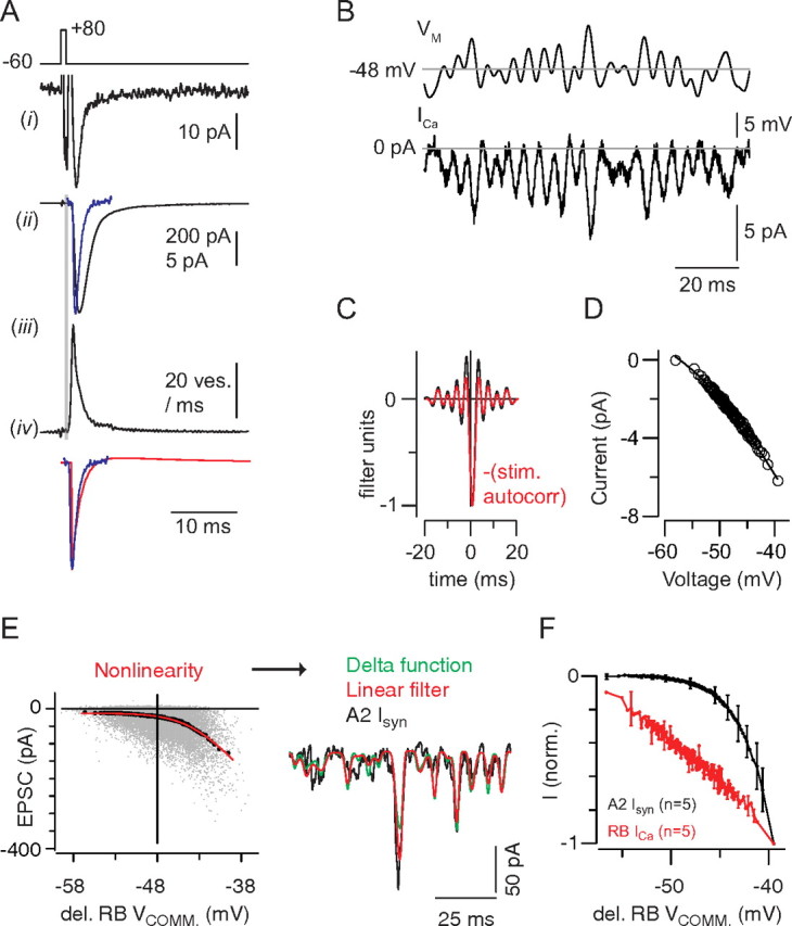
A, A Ca tail current (i) evoked by a 1 ms step from −60 to +80 mV evokes a large, fast EPSC (ii, black trace) that is slower than a quantal miniature EPSC (ii, blue trace) because of the asynchrony inherent in the release process. The extended time course of release is illustrated by deconvolving the miniature EPSC from the evoked response (iii). The gray area highlights the synaptic delay. The waveform of the quantal miniature EPSC (blue) resembles strongly the DOE (black) approximating the true linear filter of the synapse (iv). B, The Ca current elicited by the quasi-white noise stimulus. C, The linear filter exhibits a delay of ∼0.8 ms because of the time required for channel activation (black). In red, The autocorrelation of the stimulus, shifted by +0.8 ms. D, For the recording illustrated, the relationship between Ca current and voltage (delayed by 0.8 ms) was relatively linear. E, The linear prediction is generated by convolving the stimulus with a delayed Dirac delta function, in effect time-shifting (delaying) the stimulus by a constant value. The nonlinearity is represented as a function of the delayed stimulus, and the predicted output generated here (green) is almost identical with that derived from the conventional L-N analysis (B) (red; r² = 0.55 ± 0.06; n = 5 recorded pairs). F, A comparison of the Ca current and postsynaptic current nonlinearities averaged from n = 5 recordings in each case. Error bars are ±SD.

Figure 4.

Linear–nonlinear model for characterizing the RB–AII synapse. A, Schematic representation of the synaptic transfer function between presynaptic membrane potential and postsynaptic current. In both cases, synapse is partly rectifying (zero for potentials negative to rest) and otherwise linear (left) or nonlinear (right). Both a high-gain (G_HIGH) and low-gain (G_LOW) condition are shown; gain in the G_LOW condition was scaled by 0.5 (i.e., ordinate values are plotted against abscissa values multiplied by 2). Response to a +5 mV test pulse from baseline (0 mV) in the low-gain (R_LOW) and high-gain (R_HIGH) conditions are shown. Measuring gain by the ratio R_LOW/R_HIGH yields a correct 0.5 change in the linear case (A1) but an incorrect 0.25 change in the nonlinear case (A2); measuring the complete input–output function using the L-N analysis enables a scaling procedure to reveal the correct gain change in both cases (see Materials and Methods). B, The RB was stimulated with a voltage command (48 ± 3 mV) that included both repeated sequences (350 ms) and a unique sequence (4 s). A single trial is represented schematically, and a representative sample of the repeated stimulus is illustrated below. Trials were separated by 20 s. The L-N model was generated from the unique sequences and tested on the repeat sequences (i). The unique response is convolved with a linear filter (ii) to generate a linear prediction of the AII output (given in arbitrary units). This prediction is passed through a static nonlinearity (iii), characterized by strong inward rectification, to generate the L-N model of AII output. The predicted L-N output (iv) resembles the measured synaptic current (AII I_syn; averaged across six repeats; r² = 0.57 ± 0.07 for n = 5 recorded pairs). The nonlinearity shows the raw data (gray points, downsampled to 1 kHz), the binned data (black points, 200 bins), and the fit compared with the averaged response to the repeated stimulus (red line). C, The measured filter is approximated by a delayed DOE after applying a 250 Hz cutoff (fitted parameters: t_d = 2.0 ms; κ₁ = 2.6; σ₁ = 1.0 ms; κ₂ = 0.05; σ₂ = 26.6 ms). The entire L-N analysis was restricted to frequencies <250 Hz, and the measured filter was used to generate the linear prediction in B. D, Six responses to the repeated stimulus are shown to illustrate the variability of the synaptic responses. This variability gives rise to the scatter evident in the raw data (gray points) binned to generate the nonlinearity in B. The gray bars highlight responses to relatively large depolarizations; these are reproduced with considerable variability from trial to trial.

The linear filter (F) was calculated in the Fourier domain as the cross-correlation between the stimulus [s(t)] and the response [r(t); measured in picoamperes] divided by the power spectrum of the stimulus as follows:

in which s(t) is described as deviations (in millivolts) from the mean (i.e., mean of 0), s̃(ω) is the Fourier transform of s(t), r̃(ω) is the Fourier transform of r(t), * denotes the complex conjugate, and S(ω) is the power spectrum of the stimulus calculated from the autocorrelation s̃ * (ω)s̃(ω). The stimulus power was approximately flat from 0 to 250 Hz, so we calculated the filter from the numerator alone. The filter in the time domain, F(τ), was calculated by taking the inverse Fourier transform of F̃(ω). All analyses were restricted to the 250 Hz bandwidth of the stimulus and were performed in MATLAB.

In theory, the filter should be nonzero only for positive time points. The measured filter, however, showed a peak negative response at +2–3 ms with “ripples” extending on either side of the peak, including nonzero values at negative time points. Further analysis suggested that the measured filter shape arose from a faster underlying filter whose shape was affected by the 250 Hz bandwidth of the analysis. We found that the underlying filter could be modeled as a delayed difference-of-exponentials (DOE) function, d(t), that is zero up to a short delay (t_d) and then described as follows:

in which each exponential has an amplitude (κ₁ and κ₂) and a time constant (σ₁ and σ₂). When the DOE function was limited to the 250 Hz bandwidth of the analysis, it closely approximated the measured filter, including the ripples that extend to negative time points (see Fig. 4C). Thus, the measured filter apparently represented a band-limited version of an underlying filter that was too fast to measure with high accuracy. In the analysis that follows, we used the measured filter between t = −25 and +75 ms.

A linear prediction of the synaptic response, r_L(t), was generated by convolving the filter with the stimulus as follows:

At each time point, the linear prediction was plotted against the measured response to generate the static nonlinearity of the synapse, which typically showed inward rectification. We binned the data along the x-axis (200 bins) and fit the data with a smooth curve as follows:

in which C is the cumulative normal density and the parameters correspond to a maximum response (α), response gain (β), response threshold (γ), and an offset (δ) (Chander and Chichilnisky, 2001; Zaghloul et al., 2005). This nonlinear (N) function served as the “input–output” relationship that transformed the L prediction into the L-N prediction (r_LN) as follows:

We used the L-N description to compare the effect of changing either the mean (−51 vs −45 ± 3 mV) or the SD (−48 ± 1.5 vs 4.5 mV) of the RB command potential. To make this comparison, we generated an individual filter for each condition, and then fit the two nonlinearities simultaneously with three shared parameters (α, γ, δ) and one unique parameter for each N function (β₁ and β₂). The two N functions then could be aligned by “stretching” one along the x-axis by the factor β₁/β₂ (Chander and Chichilnisky, 2001; Zaghloul et al., 2005). To maintain a constant output of the L-N model, the filter had to be scaled by the same factor. Thus, the change between two conditions could be described as a difference in the filter amplitudes followed by a common N function. In one case (comparing conditions with different means), we subtracted a vertical offset in the N function before performing the alignment procedure so that the two nonlinearities were matched at f(x = 0). In this case, we could interpret the offset (i.e., tonic inward current at x = 0) as an unmodulated increase in release independent of the modulated release.

To quantify the predictive ability of the L-N model, we computed the squared correlation (r²) between the L-N prediction and the average response to the repeated stimulus (4–11 trials for each paired recording). In all cases, r² underestimates the predictive power of the model, because noise remained after averaging ∼4–11 responses. This was particularly evident in the most depolarized (V_M = −45 ± 3 mV) (see Figs. 5, 7Civ) and lowest SD (V_M = −48 ± 1.5 mV) (see Figs. 6, 7Eiv) conditions. To derive a quantitative measure of the noise, we divided the repeated responses recorded in each cell into two groups and calculated the r² between the averages of each group (i.e., we sought to determine how well each response represented the group). In all cases, the correlation between the L-N prediction and the averaged response was very close to the correlation between the averages of different subsets (model vs subsets; r² = mean ± SD): in the case of changing the mean RB command potential, the r² was 0.68 ± 0.06 versus 0.70 ± 0.16 for −51 mV and 0.12 ± 0.14 versus 0.20 ± 0.16 for −45 mV. In the case of changing the SD of the RB command potential, the r² was 0.68 ± 0.09 versus 0.72 ± 0.17 for SD of 4.5 mV and 0.14 ± 0.08 versus 0.11 ± 0.08 for SD of 1.5 mV.

Figure 5.

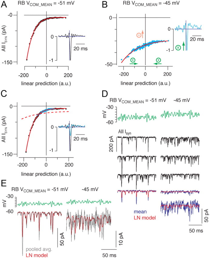
Depolarizing the rod bipolar cell membrane potential reduced synaptic gain. A, B, The static nonlinearity and linear filter (insets) are shown for conditions in which the mean rod bipolar command potential (V_{com_mean}) was either −51 (A) or −45 mV (B); in both cases, the SD of the white noise input was 3 mV. The nonlinearities were fit (red line) simultaneously by allowing a scale factor to differ between conditions. C, The nonlinearity of the depolarized mean condition could be aligned with the nonlinearity of the hyperpolarized mean condition by adding a constant (9.3 pA for this recording and 5.5 ± 2.4 pA for n = 5 paired recordings; B, orange arrow) and scaling the x-axis (by 0.36 for this recording and 0.32 ± 0.04 for n = 5 paired recordings; B, green arrows). To maintain a constant L-N model output, the filter was multiplied by the same scaling factor (inset). Depolarizing the RB reduced output gain to 36% of the gain in the hyperpolarized condition (32 ± 4% for the population of n = 5 paired recordings). The red dashed line shows the unscaled fit in the depolarized condition in B. Depolarizing the RB reduced synaptic gain. D, Three responses to repeated stimuli with means of −51 mV (left) and −45 mV (right) illustrate the variability inherent in the data. The L-N prediction is better correlated with the averaged response at −51 mV than with the averaged response at −45 mV because of the increased amount of uncorrelated release at depolarized potentials as well as the reduction in the size of the responses correlated with the stimulus. The average response in the −45 mV condition is shown both at the same scale as the −51 mV condition and on an expanded scale. E, Pooling data from n = 5 recorded pairs improves the predictive power of the L-N model. Gray trace, Response to repeated stimulus averaged across all recorded pairs; red trace, L-N prediction derived from model constructed with pooled data. r² = 0.86 and 0.72 for −51 and −45 mV, respectively.

Figure 7.

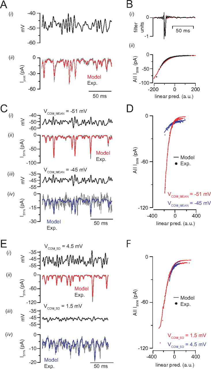
A phenomenological model of the RB–AII synapse. A, A presynaptic voltage command (top) is applied to the model to generate a simulated synaptic response (red trace, bottom). The simulated response (red) resembles the experimentally observed postsynaptic response to the same presynaptic stimulus (black; response averaged from n = 5 recorded RB–AII pairs). B, The linear filter (i) and static nonlinearity (ii) extracted from L-N analysis of the simulated output of the synapse (red) matches closely the linear filter and static nonlinearity describing the experimentally measured input–output relationship (black). C, E, The phenomenological model of the RB–AII synapse reproduces experimentally observed adaptation to stimulus mean and variance. Stimuli (i, iii) and responses (ii, iv) (black, experiment; red and blue, model) for each condition are illustrated. Experimental responses are averages from n = 5 paired recordings for each condition. D, F, Static nonlinearities derived for experimental (dots) and simulated (lines) conditions. Increasing stimulus mean from −51 to −45 mV reduced gain by 63%; raising stimulus SD from 1.5 to 4.5 mV reduced gain by 15%. For simplicity, the scaled nonlinearities are not illustrated (see Materials and Methods).

Figure 6.

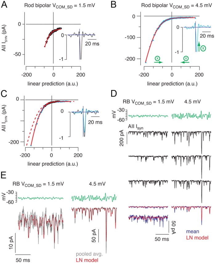
Increasing SD of the rod bipolar cell membrane potential reduces synaptic gain. A, B, The static nonlinearity and linear filter (insets) are shown for conditions in which the mean RB command potential was −48 mV, and the SD of the command potential (V_{com_SD}) was either 1.5 (A) or 4.5 mV (B). The nonlinearities were fit (red line) simultaneously by allowing a scale factor to differ between conditions. C, The nonlinearity of the high SD condition could be aligned with the nonlinearity of the low SD condition by scaling the x-axis (by 0.83; B, green arrows). To maintain a constant L-N model output, the filter is multiplied by the same scaling factor (inset). Increasing the SD of the rod bipolar reduced output gain to 83% of the gain in the low SD condition. The red dashed line shows the unscaled fit in the high SD condition in B. D, Three responses to repeated stimuli with SD of 1.5 mV (left) and 4.5 mV (right) illustrate the variability inherent in the data. The L-N prediction is better correlated with the averaged response when the modulated voltage is larger (i.e., when the proportion of release events correlated with the stimulus is higher). The average response in the low SD condition is shown both at the same scale as the high SD condition and on an expanded scale. E, Pooling data from n = 5 recorded pairs improves the predictive power of the L-N model. Gray trace, Response to repeated stimulus averaged across all recorded pairs; red trace, L-N prediction derived from model constructed with pooled data. r² = 0.70 and 0.88 for SD of 1.5 and 4.5 mV, respectively.

Given the noise arising from tonic exocytosis (i.e., desynchronous release) under some experimental conditions (see Fig. 2D), we believe that the L-N model performs as well as can be expected of any model. Its predictive ability would be improved, and it could be tested more rigorously, were larger data sets available. Because we could not obtain paired recordings lasting long enough to create larger data sets for individual RB–AII pairs, we approximated such sets by pooling the data from individual paired recordings. We did this by grouping all experimental recordings into one ensemble set and analyzing the pooled data in the same way as individual pairs: the linear filters and nonlinearities were extracted after concatenating all of the unique responses, and the L-N prediction was compared with the responses to repeated stimuli averaged across all recorded pairs. After doing this, the predictive power of the model was enhanced considerably, as expected (individual vs pooled; r² = mean): in the case of changing the mean RB command potential, the r² was 0.68 versus 0.86 for −51 mV and 0.12 versus 0.72 for −45 mV. In the case of changing the SD of the RB command potential, the r² was 0.68 versus 0.88 for SD of 4.5 mV and 0.14 versus 0.70 for SD of 1.5 mV. Thus, we conclude that the mean transfer function at the RB–AII synapse is well described by our L-N model.

Figure 2.

The strength of transmission at the RB–AII synapse is reduced by tonic presynaptic depolarization. A, The presynaptic RB is stepped to prepulse potentials between −60 and −42 mV for 750 ms before a test pulse: a 10 ms depolarization of +10 mV relative to the prepulse potential. Averaged (n = 4 responses at each potential) presynaptic Ca currents (middle) and evoked EPSCs (bottom) are illustrated. Some inactivation of the presynaptic Ca current during the prepulse is evident at −48 and −42 mV. EPSCs have been separated by a vertical offset. B, Ca currents and EPSCs are illustrated at higher temporal resolution. EPSCs are not offset. C, Summary of n = 7 experiments. Ca currents (integrated) and EPSCs (quantal contents) recorded during the test pulse from each RB–AII pair were normalized to the largest currents recorded in that pair. The magnitude of Ca influx was relatively constant following each prepulse, but evoked exocytosis was inhibited significantly by the more depolarizing prepulses. Error bars indicate SEM. D, Examples of EPSCs recorded in the 100 ms before the test pulse demonstrate both the increased exocytosis evoked by tonic depolarization (colors as in A) and our ability to resolve and evaluate individual synaptic events (denoted as vertical lines in the traces above the EPSCs). E, The EPSC amplitudes do not vary with interevent interval: amplitudes are normalized to the mean quantal EPSC amplitude (recorded in the absence of presynaptic stimulation), and data are binned in 3 ms bins. The quantal content of the EPSCs is larger than one (average mEPSC, 27.6 ± 3.1 pA), reflecting the multivesicular release that is known to occur at this synapse. The average interevent intervals at −54, −48, and −42 mV were 37.2 ± 33.8, 10.3 ± 8.7, and 4.9 ± 1.8 ms, respectively. Events were exponentially distributed, indicating that they arose from a Poisson process. The average interevent interval in the absence of stimulation was 208.9 ± 38.0 ms (n = 11 paired recordings).

Model of synapse.

Transmission at the RB–AII synapse was modeled by tracking the cycling of a presynaptic readily releasable vesicle pool (RRP) in response to altered presynaptic potential. The RRP was the mean number N of vesicles that were available for release at any point in time [maximum size N_MAX = 80 vesicles (Singer and Diamond, 2006; Zhou et al., 2006; Jarsky et al., 2010; Oltedal and Hartveit, 2010)]. Its evolution was modeled by a differential equation as follows:

The first term described the mean rate of exocytosis, with r(V(t)) being the rate of release as a function of the command voltage V(t). The second term captured the recycling of vesicles back into the RRP, with the recycling rate given by α and the effective size of the RRP given by N_∞(h).

The release rate r(V(t)) depended both on the varying instantaneous voltage and on the time-averaged voltage as follows:

r_V(V) captured the rapid modulation of release by fluctuations in the presynaptic stimulus [i.e., rapid changes in the number of open channels at each active zone (AZ)], and r_U described release that depended on the mean voltage only (reflecting the mean number of open channels at each AZ and perhaps processes like slow changes in intraterminal [Ca²⁺]) (see Fig. 2). This scheme reflects the finding that the opening of individual Ca channels controls exocytosis from RB AZs (Jarsky et al., 2010).

The voltage dependence of r_V(V) was described as the sigmoid:

V_1/2 and k were chosen to yield a curve that resembled the G–V relationship of the presynaptic Ca conductance, h captured Ca channel inactivation, and A is a fit parameter chosen to provide good agreement between instantaneous voltage and release. Again, this description relies on the observed close coupling between Ca channels and release sites at the RB AZ. A and k were constants, but V_1/2 and h varied with the mean membrane potential to approximate depolarization-induced modulation of Ca currents: namely, shifts of the activation curve to higher voltages and increases in the extent of inactivation. The evolution of V_1/2 and h were described as follows:

The time constants τ_h and τ_v1/2 = 400 ms and were derived from recorded Ca currents (see Fig. 3). Based on recorded Ca currents (see Fig. 3), V_1/2∞ was made a piecewise linear function of the mean membrane potential (Table 1). From Ca current recordings and from changes in release rate assessed by the quasi-white noise experiments, we assigned h_∞ (Table 1). V_1/2 and h were initialized at their respective steady-state levels at V = −60 mV (the holding potential of the RBs).

Figure 3.

Presynaptic Ca currents inactivate at depolarized membrane potentials in the physiological range. A1, The RB was stepped to potentials between −60 and −42 mV for 750 ms. Then, the membrane potential was ramped at 1 mV/ms to −10 mV. A2, The maximal Ca current is reduced by inactivation. B, Summary data from n = 16 RBs illustrate the reduction in maximal current (to ∼75% of control) induced by inactivation. C, Comparison of the conductance–voltage relationships recorded following prepulses to −60 (no prepulse) or −42 mV illustrates a small rightward shift in half-maximal activation potential (from −37.1 to −33.4 mV as determined by a Boltzmann sigmoid fit to the averaged data) that accompanies inactivation.

Table 1.

Parameter values for various mean potentials

	VMean ≤−54	VMean = −51	VMean = −48	VMean = −45	VMean = −42
V1/2∞(VMean)	−41	−39.5	−38	−36.5	−35
h∞(VMean)	1	1	0.87	0.48	0.18
B(VMean)	0	0	0.003	0.055	0.25

Values are expressed in millivolts.

Uncorrelated release was described as follows:

with B(V_Mean) given in Table 1. With the exception of B(−42), these values were determined empirically to approximate experimentally observed tonic inward currents during hyperpolarizing white noise stimuli. It should be noted that B(−42) and h_∞(−42) could not be constrained by the quasi-white noise experiments (see Fig. 7) because only voltage step experiments (see Fig. 8) were performed at this potential. Thus, these parameters are relatively unconstrained. B and h_∞, however, were used only for the RRP simulation (see Fig. 8C–E), and over a range of parameters our simulations fell within 1 SD of the experimental data.

Figure 8.

The RRP at the RB–AII synapse is reduced by tonic presynaptic depolarization. A, The presynaptic RB is stepped to prepulse potentials between −60 and −42 mV for 700 ms before a 5 ms step to −10 mV. Presynaptic Ca currents (middle) and evoked EPSCs (bottom) are illustrated. EPSCs have been separated by a vertical offset. B, Ca currents and EPSCs are illustrated at higher temporal resolution. EPSCs are not offset. C, Summary of n = 7 experiments. Ca currents (integrated) and EPSCs (quantal contents) recorded during the test pulse from each RB–AII pair were normalized to the largest currents recorded in that pair. D, Simulated synaptic currents generated by our phenomenological model (stimulus as in A). The inset illustrates a small, steady-state component of release at depolarized potentials. E, Simulated responses to the depolarization to −10 mV at higher temporal resolution. F, Comparison of the output of the model to the experimentally measured responses. Here, the error bars on the experimental data points are ±SD.

Because individual release sites are controlled by the openings of individual Ca channels (Jarsky et al., 2010), vesicles near inactivated Ca channels are not likely to undergo exocytosis, effectively reducing the RRP. Therefore, we took the effective size of the RRP to be the following:

Recycling of vesicles into the available pool occurred with a time constant α⁻¹ = 130 ms to approximate the steady-state rate of exocytosis that follows complete release of the RRP (Singer and Diamond, 2006).

The EPSC was determined by convolving the mean number of vesicles released in unit time r(V(t))N(t) with the experimentally measured quantal miniature EPSC (mEPSC) waveform (Jarsky et al., 2010). The mEPSC waveform was modeled as a difference of exponentials with a τ_Fast = 0.4 and τ_Slow = 0.54 and a peak amplitude of −25 pA. Additionally, the variability of release was captured by convolving release events with a Gaussian distribution of mean of 1.5 ms and SD of 0.5 ms, with negative values set to zero and the Gaussian renormalized to have an area equal to 1.

To compare the model to the experiment, we grouped all experimental recordings into one ensemble set and analyzed the pooled data in the same way that individual pairs were analyzed, as described above for the L-N analysis. There was one exception to this approach: experimentally, in the quasi-white noise experiments involving a depolarizing step to −45 mV, we often observed a burst of delayed release following the step. We did not attempt to characterize this mode of release in the model, and we compared the model only to the last 1.2 s of the 5.6 s recorded response. This 4.4 s delay allowed the surge of release to decay almost completely (τ_Decay = 1300 ms).

We took care to constrain the model parameters by experimental measurements to avoid overfitting. The only parameters used in the white noise experiments that were not strongly constrained by experimental data were those associated with the sigmoid function describing r_V: A, k, and baseline V_1/2∞ (i.e., V_1/2∞ for mean V ≤ −54 mV). To assign values to these variables, r_V(V) first was fit by eye to produce simulations consistent with experiments (see Figs. 7, 8). Afterward, a least-squares fitting procedure (constructed by using the fminsearch unconstrained nonlinear optimization tool from MATLAB) was used to verify that the chosen values for the free parameters approximated the optimal ones by minimizing the error associated with the repeated −51 ± 3 and −48 ± 4.5 mV stimuli (for which experimentally recorded responses were relatively noiseless).

Unless indicated otherwise, all values below are presented as mean ± SEM.

Results

Rod bipolar cells depolarize with increasing background illumination

In a published study, the responses of mouse RBs to flashes of light were recorded under multiple levels of background illumination (0–370 R* · rod⁻¹ · s⁻¹) (Dunn et al., 2006). Here, we report the RB membrane potential (V_M) recorded under these conditions. In darkness, the resting potential of the cells (V_REST) was −54 ± 0.2 mV (n = 23) (Pang et al., 2004). At background intensities of >1 R* · rod⁻¹ · s⁻¹, V_M depolarized to −48 mV at 10 R* · rod⁻¹ · s⁻¹ and to −41 mV at 100 R* · rod⁻¹ · s⁻¹. Thus, within the operating range of the rod bipolar cell (i.e., darkness to ∼10³ R* · rod⁻¹ · s⁻¹), RBs experience a steady membrane depolarization of up to ∼15 mV from V_REST in darkness (Fig. 1). We proceeded to examine the influence of this steady depolarization on transmission at RB synapses.

Steady-state depolarization inhibits transmission at the RB–AII synapse

First, we assessed the effect of sustained depolarization on the strength of transmission at the RB–AII synapse (Fig. 2). The RB was stepped to a prepulse potential between −60 and −42 mV (6 mV increments, spanning the physiological range) (Fig. 1) for 750 ms followed by a 10 ms +10 mV incremental test step. The prepulse to −54 mV augmented I_Ca by ∼24% and the EPSC by ∼33% (I_Ca from 0.54 ± 0.10 to 0.75 ± 0.11; EPSC from 0.54 ± 0.10 to 0.85 ± 0.11; values normalized to maximum response). This augmentation occurred because the prepulse moved V_M closer to the activation threshold for the presynaptic Ca channels. Additional increases in prepulse depolarization, however, reduced dramatically the quantal contents of the test EPSCs while exerting relatively mild effects on the presynaptic I_Ca (Fig. 2C). Thus, the gain of the RB–AII synapse—quantified here as the postsynaptic current evoked by a 10 mV depolarization—declines steeply when presynaptic V_M transits the range of potentials encountered as ambient light intensity increases from 1 to 100 R* · rod⁻¹ · s⁻¹.

The presynaptic Ca current during the test pulse exhibited some inactivation and was reduced to 34 ± 2.5% of the peak following the most depolarized prepulse (Fig. 2A) (discussed in detail below). Because the release of individual vesicles at the RB presynaptic AZ is coupled to the opening of single Ca channels, the quantal contents of the EPSCs vary linearly with the amplitudes of the presynaptic Ca currents (Jarsky et al., 2010). Therefore, the observed reductions in the quantal contents of the EPSCs elicited by the most depolarizing prepulse are significantly greater—more than twice so—than would be predicted simply from a reduction in presynaptic Ca²⁺ influx (Fig. 2C).

AMPA receptor desensitization does not contribute to the attenuation of EPSCs evoked at depolarized RB membrane potentials

We tested whether AMPAR desensitization contributed to the attenuation of EPSCs measured here. We plotted the amplitudes of EPSCs occurring in the 200 ms before the test step against their interevent intervals: because the AMPARs on AIIs recover from desensitization quite quickly [τ_recovery = 12.5 ms (Veruki et al., 2003)], any effects of desensitization arising from sustained exocytosis on the EPSC would be most evident when the time between EPSCs evoked at the same AZ was short (Fig. 2D,E) (Otis et al., 1996; Singer and Diamond, 2006). The measured interevent intervals were exponentially distributed, as would be expected for a Poisson process (data not shown). Furthermore, EPSC amplitudes were remarkably constant as the interevent interval varied (Fig. 2E). The interevent interval, reflecting release from all presynaptic AZs, was shortest at the most depolarized potential (varying from 37.2 ± 10.1 ms at −54 mV to 4.9 ± 0.5 ms at −42 mV; it was 208.9 ± 38.0 ms in the absence of presynaptic stimulation; n = 11 paired recordings). At a single AZ, however, this interval would be ∼10 times longer [∼50 ms at −42 mV, given that a single RB makes 10 synapses onto a single AII (Tsukamoto et al., 2001)].

Several factors appear to prevent AMPAR desensitization from shaping the EPSCs at this synapse. First, the minimal average interevent interval at a single AZ is approximately four times longer than τ_recovery. Second, the τ_decay of the EPSC waveform approximates the τ_deactivation of the AMPAR (∼1 ms), which is much faster than the τ_{desensitization} (Singer and Diamond, 2003; Veruki et al., 2003). Furthermore, the spatiotemporal profile of the glutamate concentration change in the study of AMPAR desensitization performed using somatic membrane patches (3 mm, 1 ms square pulse) is likely higher and longer than that found at an RB–AII synapse following the exocytosis of one or two vesicles (Clements, 1996; Veruki et al., 2003). As a consequence, the opportunities for AMPAR desensitization during synaptic transmission are likely limited. Thus, echoing previous studies (Singer et al., 2004; Singer and Diamond, 2006), we conclude that AMPAR desensitization does not contribute to use-dependent depression of EPSCs arising at the RB–AII synapse.

Presynaptic Ca currents exhibit voltage-dependent inactivation

From the recordings in Figure 2A, it was apparent that the presynaptic Ca currents inactivated over the course of the 750 ms prepulse. Inactivation was not evident during the step to −54 mV, but it was observed during the step to −48 mV and was most prominent during the step to −42 mV (Fig. 3A). Because a reduction in Ca²⁺ influx will reduce exocytosis independently from any diminution in the RRP size, we thought it important to determine the steady-state reduction in Ca channel availability that occurs when the RB is depolarized tonically. To do this, we depolarized RBs to potentials between −54 and −42 mV for 750 ms and then ramped the membrane potential to −10 mV at a rate of 1 mV/ms (i.e., much faster than the rate of current inactivation but slow enough to allow channels to activate at all potentials) (Fig. 3A) (von Gersdorff and Matthews, 1996; Rabl and Thoreson, 2002). At −42 mV, the Ca current inactivated with a τ = 393 ± 65 ms to 34 ± 2% of its initial peak (n = 16). This slow and incomplete inactivation is consistent with reports of Ca²⁺-dependent inactivation of Ca currents at other retinal ribbon synapses (von Gersdorff and Matthews, 1996; Rabl and Thoreson, 2002).

As demonstrated by the instantaneous current–voltage relationships (Fig. 3B), the peak of the ramp-activated Ca current was reduced by ∼25% (to 76 ± 3% of control; n = 16) following the step to −42 mV (Fig. 3B). Thus, a tonic depolarization of the magnitude evoked by background light reduced Ca channel availability. The current–voltage relationships derived from the ramp stimulus were converted into conductance–voltage relationships (assuming an E_Ca of 90 mV) (Fig. 3C) and used in the synapse model described below. From these relationships, it was apparent that tonic depolarization induced a rightward shift (to depolarized potentials) in the voltage dependence of Ca channel activation: the half-maximal activation potential increased from −37.1 to −33.4 mV (based on curves fit to the data averaged from n = 16 recorded RBs). This shift is consistent a change in channel open probability following Ca²⁺-dependent inactivation (Imredy and Yue, 1994).

A linear–nonlinear model describes the RB–AII synaptic transfer function

Having determined that the strength of transmission at the RB–AII synapse is affected by steady-state depolarization of the presynaptic RB, next we used a L-N cascade analysis to characterize the transfer function of the synapse and to quantify further presynaptic membrane potential-dependent changes in synaptic gain (see Materials and Methods). This approach has a number of advantages over the more conventional analysis using a brief test pulse (Fig. 2). First, the L-N analysis uses a stimulus that spans a wide range of temporal frequencies so that any temporal filtering by the synapse can be characterized and compared between conditions. Second, the L-N analysis characterizes the full input–output function of the synapse because the stimulus spans a wide range of presynaptic V_M. By mapping the input–output relationship of the synapse continuously over this range, the L-N analysis accurately measures a gain change between two conditions; a limited sampling of presynaptic potentials and postsynaptic responses with test pulses can yield divergent estimates of the gain change depending on the degree of nonlinearity at the synapse (Fig. 4A). Furthermore, the L-N analysis used here is identical with the analysis used to characterize gain changes during visual stimulation of retinal neurons. Thus, the L-N analysis facilitates comparison between our study of a bipolar synapse and many previous studies of light-dependent changes in response gain (Chichilnisky, 2001; Demb, 2008; Wang et al., 2011).

A RB was stimulated with a randomly fluctuating voltage command of −48 ± 3 mV (mean ± SD; Gaussian white noise low-pass filtered with a 250 Hz cutoff frequency) to evoke exocytosis, which was assayed as EPSCs recorded in the AII. We generated a linear filter by cross-correlating the presynaptic voltage command and the evoked postsynaptic current (Fig. 4B) (see Materials and Methods). Convolving the measured filter with the bipolar cell voltage command created the linear prediction of the postsynaptic response, which was plotted against the recorded postsynaptic currents to generate the nonlinear component of the synaptic transfer function. Data were binned and fit with a smooth function (Fig. 4B) (see Materials and Methods). This nonlinearity captures the strong inward rectification of the synapse: the release rate can be increased substantially by depolarizing the presynaptic membrane, but the release rate cannot be decreased below zero.

In this L-N analysis, the linear filter reflects the frequency response of the synapse. The filters we calculated showed negative peaks at ∼2–3 ms, reflecting the brief synaptic delay. Furthermore, we observed minor ripples on either side of the peaks, and additional analysis revealed that the shape of the measured filters resulted from the limited bandwidth of the stimulus (250 Hz) (see Materials and Methods): a fast filter, such as a delayed DOE, yielded a filter time course that, when limited by the 250 Hz cutoff, resembled closely the measured filters (Fig. 4C). We conclude that the linear filter of the synapse is extremely fast and likely resembles a DOE. Because our analysis is limited by the stimulus bandwidth (250 Hz), the true underlying filter (e.g., a DOE) and the measured filter will yield the same linear prediction (because their frequency components are identical across the 250 Hz bandwidth) (see Materials and Methods). The implications of the filter shape are discussed below (see Biophysical basis of the L-N model).

Scaling the linear prediction by the nonlinearity generated a predicted output (the L-N prediction). As illustrated in Figure 4B, the L-N prediction corresponded well to the recorded data. We assessed the predictive power of the L-N model by comparing the L-N prediction to the average response to a repeated stimulus (4–11 repeats to reduce noise) (Fig. 4D). The L-N model explained 57% of the variance in the average (r² = 0.57 ± 0.07; n = 5 recorded pairs). The r² value, however, underestimates the predictive value of the L-N model when it is applied to individual paired recordings due to the significant trial-to-trial variability in the postsynaptic response. Because the number of repeats that could be averaged was limited by the recording duration, this variability was not eliminated from the averaged response. The fit to the data of the L-N prediction was enhanced considerably after pooling data from all recorded cell pairs in a given condition (see Materials and Methods). On a single trial, the EPSCs reflect a combination of exocytosis modulated by the presynaptic voltage command and tonic unmodulated exocytosis (i.e., desynchronous release) (Fig. 2), which represents the major noise source in our analysis. The total response in a given condition, then, represents a ratio between these two components of release. Conditions that decreased the ratio between modulated and desynchronous release degraded the r² value calculated for individual cell paired recordings; however, the r² values increased considerably (to 0.7–0.9) (see Materials and Methods) when predicting the response averaged across cell pairs. Thus, the L-N model could be used under experimental conditions with relatively low signal-to-noise.

Synaptic gain is reduced by depolarizing the presynaptic membrane

Changes in the local statistics in a visual scene alter the stimulus–response relationships of retinal neurons (Dunn and Rieke, 2006). Consequently, we wanted to determine how the transfer function of the RB–AII synapse varied with the statistics of the presynaptic V_M. First, we varied the mean V_M: the quasi-white noise stimulus was modulated (SD of 3 mV) around means of −51 and −45 mV. These mean potentials represent the approximate RB V_M at backgrounds of 1 and 30 R* · rod⁻¹ · s⁻¹, respectively (Fig. 1). Both conditions showed similar linear filters and rectifying nonlinearities, although the amplitudes of the postsynaptic responses were reduced markedly at the depolarized mean potential (Fig. 5A,B, insets; C). To exclude the possibility that AMPAR desensitization contributed significantly to the diminution of the postsynaptic responses evoked by the stimulus with mean of −45 mV, we repeated our analysis of EPSC amplitudes and intervals (Fig. 2D,E) and determined that the EPSC amplitudes did not vary with the interevent intervals during the quasi-white noise stimulus (data not shown). Thus, AMPAR desensitization apparently does not occur following tonic depolarization of the presynaptic membrane, and therefore we interpret changes in the postsynaptic response as reflecting a presynaptic phenomenon.

Relative to that at mean of −51 mV, the zero-crossing point of the nonlinearity was shifted by −5.5 ± 2.4 pA at mean of −45 mV (n = 5) (Fig. 5C). This −5.5 pA is the average amplitude of a tonic inward current arising from a small burst of delayed exocytosis that began ∼100 ms following the membrane depolarization to −45 mV and that decayed with a time constant of ∼1.3 s. This delayed exocytosis, which was not present at −51 mV, is likely equivalent to the desynchronous release that has been described previously (Singer and Diamond, 2003). Delayed exocytosis was not modulated by the quasi-white noise stimulus, and its presence did not alter our ability to estimate the synaptic transfer function with L-N analysis. Consequently, the difference in the zero-crossing point was subtracted from the nonlinearity before further analysis (Fig. 5B) (see Materials and Methods).

The suppression of RB output reflects a reduction in synaptic gain. We quantified the gain change by fitting the two nonlinearities with a function that included a scaling factor. Altering the scaling factor “compressed” the nonlinearity for the depolarized condition along the x-axis. This compression reflects a change in the linear prediction and therefore must be accompanied by an identical scaling of the amplitude of the linear filter (to keep the output constant of the L-N model) (see Materials and Methods). Following the scaling procedure (Fig. 5C), the nonlinearity was identical in the two conditions, and the gain change was reflected by the ratio of filter amplitudes. On average, the gain in the depolarized condition was 32 ± 4% (mean ± SEM; n = 5) of the gain in the hyperpolarized condition (i.e., the 6 mV depolarization reduced gain of synaptic transmission by ∼68%).

To explore the mechanism underlying the observed reduction in gain, we compared the total amount of exocytosis in the two experimental conditions by integrating the postsynaptic currents. Surprisingly, the charge transfer in the depolarized condition was increased by only 23 ± 12% relative to the hyperpolarized condition. The reduced gain, then, did not reflect a dramatic reduction in exocytosis. Rather, the reduced gain could be understood, at least in part, as an increase in the ratio of unmodulated (desynchronized release) to modulated release. This shift to unmodulated release both reduces the gain of modulated synaptic transmission and increases synaptic noise.

Synaptic gain is reduced by increasing the variance in presynaptic V_M

Next, we assayed the effects of changing the temporal variance of the RB voltage on synaptic gain. We used two quasi-white noise stimuli with the same mean (−48 mV) but different SDs (1.5 or 4.5 mV) (Fig. 6). Using the L-N analysis described above, we quantified the effect of the increased SD on gain. Increasing the SD did not alter significantly the zero-crossing of the nonlinearity (difference of −0.58 ± 0.71 pA; n = 5), suggesting that increased SD was not accompanied by an increase in desynchronous release. Increasing the SD, however, reduced the gain of synaptic transmission to 82 ± 1% of the gain in the low SD condition (n = 4; one outlier removed; 87 ± 10% with outlier included) (Fig. 6C). Thus, tripling the SD of the RB V_M reduced the gain of synaptic transmission by ∼18%.

A phenomenological model of the synapse reproduces the observed gain control

The RB–AII synapse exhibits profound short-term depression that arises from RRP depletion (Singer and Diamond, 2006). Because a use-dependent reduction in synaptic strength is postulated to mediate the adaptation to background light intensity exhibited at this synapse (Dunn and Rieke, 2008), we constructed a phenomenological model of the synapse to assess the contributions of RRP size and Ca channel inactivation to the gain changes revealed by our L-N analysis (see Materials and Methods).

First, we simulated the response to steady-state depolarization to −48 ± 3 SD. As illustrated by Figure 7A, the model generated a prediction that matched quite closely the experimental data (assessed by comparing the model to the response averaged across RB–AII pairs; r² = 0.93). Subjecting the simulated postsynaptic current to the L-N analysis generated a linear filter and a static nonlinearity almost identical with those arising from recorded postsynaptic currents (Fig. 7B). Next, we simulated responses to stimuli in which either the mean or variance was altered (Figs. 5, 6). Again, the model was able to reproduce accurately the postsynaptic current recorded in response to these stimuli (r² = 0.94 and 0.53 for the hyperpolarized and depolarized mean V_M experiments, respectively; r² = 0.92 and 0.70 for the high and low SD experiments, respectively) (Fig. 7C,E). The static nonlinearities calculated from these simulated data sets resembled strongly those derived from experiments (Fig. 7D,F). Scaling these nonlinearities (Figs. 5, 6) (see Materials and Methods) allowed us to quantify the gain changes arising from each manipulation of the stimulus. Gain was reduced by 64% by depolarizing the mean from −51 to −45 mV, and it was reduced by 15% by increasing the stimulus SD from 1.5 to 4.5 mV (compared with 68 and 18% for the experimental responses to the same manipulations).

Examination of the model indicated that the average size of the simulated RRP [N_∞(h) in Eq. 12 (see Materials and Methods)] was lower when the gain was reduced: it was 48 versus 4 vesicles when the mean V_M changed and 33 versus 19 vesicles when the V_M SD changed. In the case of presynaptic depolarization, our simulation indicates that unmodulated (i.e., desynchronized) release depletes the RRP, leaving few release sites available to be modulated by the stimulus. It is interesting to note that this effect of unmodulated release becomes evident at a presynaptic V_M (−45 mV) at which the average number of open Ca channels/AZ ≈ 1 (Jarsky et al., 2010): because coupling between Ca channels and release sites at the RB AZ is so efficient, continuous openings involving small numbers of channels will drive tonic exocytosis that reduces the number of vesicles available to be released in response to a transient stimulus. In the case of changing V_M SD, our simulation indicates simply that large voltage excursions deplete the RRP when these excursions occur at a higher rate than vesicle replenishment.

We wanted to assess the accuracy with which the model predicted the size of the cycling RRP. To do this, we performed an experiment in which we evoked exocytosis with a 5 ms step to −10 mV [sufficient to elicit release of the entire RRP (Singer and Diamond, 2006; Jarsky et al., 2010)] following 700 ms prepulses to potentials between −60 and −42 mV (Fig. 8A). With increasingly depolarizing prepulses, the quantal content of the evoked EPSC was reduced substantially (to ∼20% of control) (Fig. 8C). It is notable that the cell pair-to-cell pair variability in the EPSCs elicited following the depolarized prepulses was large, and the recording illustrated in Figure 8B showed the least depression (note the error bars in Fig. 8F). Significantly, RRP was not depleted completely by this stimulus: vesicles were available after 700 ms of sustained release to encode additional depolarization. The model reproduced accurately the recorded EPSCs (Fig. 8D–F). Notably, the initial responses of the model were transient in nature even though they did not reflect the release of the entire RRP. Rather, the postsynaptic response decayed rapidly after vesicle release was initiated because the rate of vesicle replenishment is much slower than that of exocytosis. This observation suggests that the transient nature of transmission at the RB–AII synapse arises from the dynamics of vesicle recycling (i.e., EPSCs always exhibit a transient component, even when the RRP has not been depleted completely) (Snellman et al., 2009). It is worth noting that, in this respect, EPSCs recorded from mouse AIIs at physiological temperatures differ from those recorded in rat AIIs at room temperature (Singer and Diamond, 2003).

Biophysical basis of the L-N model

The close correspondence between the predictions of the L-N model (which does not identify explicitly any biological mechanisms) and the phenomenological model (which reproduces the recorded data with only a few parameters) allows us to describe the cellular mechanisms that dominate the transfer function of the RB–AII synapse. In the L-N analysis, the linear filter, which resembled a delayed DOE (Fig. 4C), represents the impulse response of the system. In previous studies of this synapse, we have approximated a biological impulse response by evoking large, fast EPSCs in an AII by eliciting a Ca tail current in the presynaptic RB (Singer and Diamond, 2003; Jarsky et al., 2010). Although fast, these EPSCs are slower than the DOE probably because of the asynchrony inherent in the release process (Fig. 9A). The DOE, however, resembles the time course of a quantal miniature EPSC: the postsynaptic response to a single vesicle. Thus, the temporal filtering at this synapse reflects the time required to transform a change in synaptic glutamate concentration into a postsynaptic conductance change. The slightly biphasic shape of the DOE suggests that the release process shows attenuated sensitivity to low temporal frequencies.

To examine the biophysical basis for the delay of the DOE, we used an L-N analysis to study the transfer between RB membrane potential and the Ca current (measured as the difference current in the presence and absence of 100 μm Cd²⁺) evoked by modulating the RB command potential (−48 ± 3 mV) (Fig. 9B). The derived linear filter showed a peak at 0.8 ms with ripples on either side (Fig. 9C). Furthermore, the linear filter resembled the delayed autocorrelation of the stimulus, indicating that, when limited by the 250 Hz bandwidth of the stimulus and analysis, the transformation from presynaptic voltage to presynaptic Ca²⁺ influx is well represented as a 0.8 ms delay. Thus, the total delay reflected in the linear filter at the RB–AII synapse (i.e., the DOE delayed by 2–3 ms) combines the delay of Ca channel activation (∼0.8 ms) (Fig. 9B) and the delay in exocytosis following Ca²⁺ entry into the presynaptic terminal [∼1.5 ms (Fig. 9A) (Jarsky et al., 2010)].

The nonlinear stage between RB voltage and Ca²⁺ current was nearly linear over the voltage range tested (−58 to −38 mV) (Fig. 9D). To compare this nonlinearity to the current–voltage (I–V) relationship of synaptic release, we generated a second L-N model of the RB–AII synapse. The delayed DOE approximation of the linear filter, in the standard analysis above, showed that the filter at the synapse is very fast and that filtering in the 0–250 Hz range is minimal. We therefore approximated the filter as a simple Dirac delta function shifted 2–3 ms time (matching the peak of the standard filter measured by cross-correlation) (see Materials and Methods). In this case, the nonlinearity plots the time-shifted RB command potential versus the postsynaptic current, yielding a current–voltage (I–V) relationship for the synapse; the predictive ability of this model (r² = 0.55 ± 0.06; n = 5 recorded pairs) was nearly the same as the standard model (r² = 0.57 ± 0.07). The I–V relationship of the synapse is clearly more strongly rectifying than that of the Ca current measured over the same voltage range (Fig. 9D,E).

We conclude that multiple mechanisms likely underlie the nonlinearity at the RB synapse derived from our analysis. Although we cannot assess the individual contributions of the many nonlinear processes involved in synaptic transmission (e.g., the Ca²⁺ dependence of exocytosis), we can exclude the voltage dependence of Ca channel opening as accounting for the nonlinearity. The fact that the nonlinearities at the synapse maintain their shapes when the synaptic gain changes dramatically (Figs. 5, 6) indicates that the gain change probably occurs before the nonlinearity. To a first approximation, this excludes changes to highly nonlinear processes (e.g., the Ca²⁺-dependent steps in exocytosis) from participating in the gain change. Rather, a reduction in the number of release sites available to participate in exocytosis, arising from a diminution in the number of available vesicles and Ca channels, lowers synaptic gain.

Discussion

The time-varying distribution of retinal bipolar cell V_M changes with the visual scene, thereby altering transmission from bipolar cells and inducing the adaptations to background and contrast measured in postsynaptic neurons (Manookin and Demb, 2006; Beaudoin et al., 2007; Dunn et al., 2007; Dunn and Rieke, 2008). Here, we examined how the mean or variance of presynaptic V_M modulates the gain of transmission at the RB–AII synapse. A 6 mV depolarization within the physiological operating range of the RB reduced synaptic gain by ∼65% as a result of RRP depletion and Ca channel inactivation. Increasing the time-varying SD of V_M threefold reduced synaptic gain by ∼18%; this reduction was explained by RRP depletion alone. Our study elucidates how simple presynaptic mechanisms adjust the gain of transmission at retinal synapses on a rapid timescale to match the statistics of a changing visual scene.

A biophysical mechanism for synaptic gain control

Synaptic transmission at bipolar cell synapses has been studied extensively (for review, see Matthews, 1999; von Gersdorff and Matthews, 1999; Sterling and Matthews, 2005; Matthews and Fuchs, 2010). Studies that characterized phasic release described fundamental properties of the synapses (e.g., RRP sizes). In these studies, exocytosis was evoked using brief voltage steps to potentials more depolarized than those experienced during visual stimulation, and tonic exocytosis was suppressed by hyperpolarizing the neurons between steps. Although these studies demonstrated that RB and other bipolar cell synapses exhibit profound paired-pulse depression that arises primarily from RRP depletion (Mennerick and Matthews, 1996; von Gersdorff and Matthews, 1997; Singer and Diamond, 2006), it is difficult to extend these results and make quantitative predictions about the degree of RRP depletion during physiological function, in which V_M is modulated in a narrow range (∼10–20 mV) around the resting potential (Fig. 1), and Ca channel gating and exocytosis occur tonically.

Therefore, we quantified synaptic gain changes at the RB synapse elicited by tonic presynaptic depolarizations comparable with those evoked by visual stimulation. We complemented this analysis with a realistic model of the presynaptic AZ. Our model attributes gain changes observed following changes in the mean or variance of V_M, in part, to a common mechanism: a reduction in the RRP (Fig. 7). Thus, vesicle recycling rate limits the number of available vesicles during periods of depolarization: as the presynaptic membrane spends more time at depolarized potentials (because of either a depolarized mean potential or frequent large, transient depolarizations), the RRP shrinks and synaptic gain is reduced (Jackman et al., 2009).

To estimate the relative contributions of Ca channel inactivation and RRP depletion to the gain changes observed, we predicted synaptic output when inactivation was included or excluded as a feature of the model (i.e., variable h = 1 for all mean V_M) (see Materials and Methods). Postsynaptic mechanisms were not included in the model because AMPARs are neither saturated nor desensitized by ongoing synaptic transmission under the experimental conditions considered (Fig. 2D,E) (Singer et al., 2004; Singer and Diamond, 2006; Singer, 2007; Jarsky et al., 2010). Additionally, although the interplay between feedforward excitation and feedback inhibition certainly will contribute to regulating the responses of postsynaptic neurons during visual processing in the intact circuit (Li et al., 2007), here we did not consider the modulatory effects that inhibitory inputs onto the RB terminal may exert on synaptic gain.

Adaptation to variance was attributable to RRP depletion alone: the gain change induced by increasing stimulus SD was unaffected by removing the inactivation parameter from the model (gain change, 15% in both cases). This finding is consistent with the experimental observation that Ca currents show little inactivation at −48 mV (Figs. 3, 6). Furthermore, transient (≪100 ms) voltage excursions from −48 mV should not cause substantial Ca channel inactivation because the time constant for inactivation is slow (∼400 ms). Accordingly, Ca channel inactivation did not contribute to synaptic depression at RB synapses when depolarizing stimuli were relatively brief (<100 ms) (Singer et al., 2004; Singer and Diamond, 2006).

Ca channel inactivation contributed to adaptation to the mean. At mean V_M > −48 mV, inactivation of recorded presynaptic Ca currents was evident (steady-state/peak, 0.34 at −42 mV) (Fig. 3). Consequently, removing the inactivation feature of the model altered both the simulated responses and the gain change arising from depolarizing mean V_M from −51 to −45 mV: the gain change was 63% with inactivation present (resembling the experimental effect) but only 37% with inactivation absent. Furthermore, the simulated response to a quasi-white noise stimulus of mean V_M = −45 mV failed to reproduce the experimental response without inactivation present: large stimulus fluctuations evoked large postsynaptic responses, and these responses became better correlated with the stimulus than were the experimental ones (i.e., more vesicles were available for correlated release) (see Materials and Methods).

Simplistically, the reduced gain of the model at the depolarized V_M (0.37) is a function of two factors: RRP depletion (0.63; taken from the simulation with Ca channel inactivation absent) and Ca channel inactivation (0.37/0.63 = 0.59). Thus, Ca channel inactivation and RRP depletion may affect gain similarly: at RB synapses, exocytosis varies linearly with the number of open channels because of the close coupling between channels and release sites (Jarsky et al., 2010). Consequently, lowering Ca current amplitude will generate a proportional reduction in synaptic release (Jarsky et al., 2010). This differs from observations of conventional synapses like the calyx of Held, at which coupling between Ca channels and release sites is looser, and a small change in Ca channel availability generates large changes in the number of vesicles released (Xu and Wu, 2005).

Relevance to visual processing

Here, we tested the effect of “pure” changes in either the mean or SD of RB V_M on synaptic gain (Figs. 5, 6). We did not intend to reproduce accurately RB responses to particular visual scenes; rather, we used our analytical approach to assess how well defined changes in presynaptic V_M affected the synaptic transfer function. In reality, the mean and SD of V_M change simultaneously, especially at scotopic intensities (for review, see Dunn et al., 2007). For example, when only one of the ∼20 rods presynaptic to an RB (Tsukamoto et al., 2001) absorbs a single photon within the integration time of the rods (∼100 ms), contrast is almost impossible to define (i.e., it is either 0 or 100%). Increasing the mean intensity, then, will depolarize the RB and increase fluctuations in V_M. Under these conditions, changes in the mean and SD of RB V_M will combine to generate synaptic gain control.

Our study suggests that the ability to adapt to contrast is an intrinsic property of RB—and by extension, all bipolar cell—synapses. Under conditions in which bipolar cells can detect contrast [>10 R* · rod⁻¹ · s⁻¹ (Beaudoin et al., 2008)], their individual synapses should adapt at high contrast, without requiring network interactions, and generate adaptive responses in postsynaptic neurons (Brown and Masland, 2001; Manookin and Demb, 2006; Beaudoin et al., 2007). The experimental data and simulations presented here, however, do not preclude contributions from other cellular mechanisms resident to bipolar cells.

In the salamander retina, fast-onset contrast adaptation observed in ganglion cells is proposed to arise from a Ca²⁺-dependent mechanism that adjusts the responses of the presynaptic bipolar cells to photoreceptor input (Rieke, 2001). This mechanism may be modified further by the intrinsic membrane properties of the bipolar cells (Mao et al., 1998). Thus, in the future it will be important to determine whether gain control mechanisms exist in mammalian bipolar cell somata and dendrites and how they interact with the synaptic mechanism described here. Furthermore, it is notable that the mechanisms underlying background adaptation in (ON-type) RBs may not contribute to adaptation in OFF cone bipolar cells, because elevated background luminance should hyperpolarize OFF cells.

A 45% reduction in gain at RB–AII synapses was observed with small increases in background luminance (1 R* · rod⁻¹ · s⁻¹) that evoked only ∼2 mV presynaptic depolarizations [to V_M ≈ −52 mV (Fig. 1) (Dunn and Rieke, 2008)]. Under these conditions, the gain change likely depended on RRP depletion alone, as we observed very little Ca channel inactivation at V_M < −51 mV (Fig. 3). Ca channel inactivation became evident only during tonic depolarization to more positive potentials (Fig. 3) (corresponding to a background ≈10 R* · rod⁻¹ · s⁻¹ in Fig. 1), suggesting that Ca channel inactivation may broaden the operating range of the RB synapse by limiting RRP depletion during tonic depolarization elicited by backgrounds of 10–100 R* · rod⁻¹ · s⁻¹ (in the range of V_M examined here) (Figs. 5, 7). It is notable that the observed approximately threefold reduction in gain following presynaptic depolarization from −51 to −45 mV (Fig. 5) (the change in V_M corresponded to a change from 1 to 10–20 R* · rod⁻¹ · s⁻¹ in background light intensity as illustrated in Fig. 1) approximated the approximately threefold reduction in the gain of the AII light response at background light intensities between 1 and 10 R* · rod⁻¹ · s⁻¹ (Dunn et al., 2006).

References

- Baccus SA, Meister M. Fast and slow contrast adaptation in retinal circuitry. Neuron. 2002;36:909–919. doi: 10.1016/s0896-6273(02)01050-4. [DOI] [PubMed] [Google Scholar]
- Beaudoin DL, Borghuis BG, Demb JB. Cellular basis for contrast gain control over the receptive field center of mammalian retinal ganglion cells. J Neurosci. 2007;27:2636–2645. doi: 10.1523/JNEUROSCI.4610-06.2007. [DOI] [PMC free article] [PubMed] [Google Scholar]
- Beaudoin DL, Manookin MB, Demb JB. Distinct expressions of contrast gain control in parallel synaptic pathways converging on a retinal ganglion cell. J Physiol. 2008;586:5487–5502. doi: 10.1113/jphysiol.2008.156224. [DOI] [PMC free article] [PubMed] [Google Scholar]
- Brown SP, Masland RH. Spatial scale and cellular substrate of contrast adaptation by retinal ganglion cells. Nat Neurosci. 2001;4:44–51. doi: 10.1038/82888. [DOI] [PubMed] [Google Scholar]
- Chander D, Chichilnisky EJ. Adaptation to temporal contrast in primate and salamander retina. J Neurosci. 2001;21:9904–9916. doi: 10.1523/JNEUROSCI.21-24-09904.2001. [DOI] [PMC free article] [PubMed] [Google Scholar]
- Chichilnisky EJ. A simple white noise analysis of neuronal light responses. Network. 2001;12:199–213. [PubMed] [Google Scholar]
- Clements JD. Transmitter time course in the synaptic cleft: its role in central synaptic function. Trends Neurosci. 1996;19:163–171. doi: 10.1016/s0166-2236(96)10024-2. [DOI] [PubMed] [Google Scholar]
- Demb JB. Functional circuitry of visual adaptation in the retina. J Physiol. 2008;586:4377–4384. doi: 10.1113/jphysiol.2008.156638. [DOI] [PMC free article] [PubMed] [Google Scholar]
- Dunn FA, Rieke F. The impact of photoreceptor noise on retinal gain controls. Curr Opin Neurobiol. 2006;16:363–370. doi: 10.1016/j.conb.2006.06.013. [DOI] [PubMed] [Google Scholar]
- Dunn FA, Rieke F. Single-photon absorptions evoke synaptic depression in the retina to extend the operational range of rod vision. Neuron. 2008;57:894–904. doi: 10.1016/j.neuron.2008.01.031. [DOI] [PMC free article] [PubMed] [Google Scholar]
- Dunn FA, Doan T, Sampath AP, Rieke F. Controlling the gain of rod-mediated signals in the mammalian retina. J Neurosci. 2006;26:3959–3970. doi: 10.1523/JNEUROSCI.5148-05.2006. [DOI] [PMC free article] [PubMed] [Google Scholar]
- Dunn FA, Lankheet MJ, Rieke F. Light adaptation in cone vision involves switching between receptor and post-receptor sites. Nature. 2007;449:603–606. doi: 10.1038/nature06150. [DOI] [PubMed] [Google Scholar]
- Gollisch T, Meister M. Eye smarter than scientists believed: neural computations in circuits of the retina. Neuron. 2010;65:150–164. doi: 10.1016/j.neuron.2009.12.009. [DOI] [PMC free article] [PubMed] [Google Scholar]
- Imredy JP, Yue DT. Mechanism of Ca2+-sensitive inactivation of L-type Ca2+ channels. Neuron. 1994;12:1301–1318. doi: 10.1016/0896-6273(94)90446-4. [DOI] [PubMed] [Google Scholar]
- Jackman SL, Choi SY, Thoreson WB, Rabl K, Bartoletti TM, Kramer RH. Role of the synaptic ribbon in transmitting the cone light response. Nat Neurosci. 2009;12:303–310. doi: 10.1038/nn.2267. [DOI] [PMC free article] [PubMed] [Google Scholar]
- Jarsky T, Tian M, Singer JH. Nanodomain control of exocytosis is responsible for the signaling capability of a retinal ribbon synapse. J Neurosci. 2010;30:11885–11895. doi: 10.1523/JNEUROSCI.1415-10.2010. [DOI] [PMC free article] [PubMed] [Google Scholar]
- Kim KJ, Rieke F. Temporal contrast adaptation in the input and output signals of salamander retinal ganglion cells. J Neurosci. 2001;21:287–299. doi: 10.1523/JNEUROSCI.21-01-00287.2001. [DOI] [PMC free article] [PubMed] [Google Scholar]
- Li GL, Vigh J, von Gersdorff H. Short-term depression at the reciprocal synapses between a retinal bipolar cell terminal and amacrine cells. J Neurosci. 2007;27:7377–7385. doi: 10.1523/JNEUROSCI.0410-07.2007. [DOI] [PMC free article] [PubMed] [Google Scholar]
- Manookin MB, Demb JB. Presynaptic mechanism for slow contrast adaptation in mammalian retinal ganglion cells. Neuron. 2006;50:453–464. doi: 10.1016/j.neuron.2006.03.039. [DOI] [PubMed] [Google Scholar]
- Mao BQ, MacLeish PR, Victor JD. The intrinsic dynamics of retinal bipolar cells isolated from tiger salamander. Vis Neurosci. 1998;15:425–438. doi: 10.1017/s0952523898153051. [DOI] [PubMed] [Google Scholar]
- Marmarelis PZ, Naka KI. Nonlinear analysis and synthesis of receptive-field responses in the catfish retina. II. One-input white-noise analysis. J Neurophysiol. 1973;36:619–633. doi: 10.1152/jn.1973.36.4.619. [DOI] [PubMed] [Google Scholar]
- Matthews G. Synaptic mechanisms of bipolar cell terminals. Vision Res. 1999;39:2469–2476. doi: 10.1016/s0042-6989(98)00249-1. [DOI] [PubMed] [Google Scholar]
- Matthews G, Fuchs P. The diverse roles of ribbon synapses in sensory neurotransmission. Nat Rev Neurosci. 2010;11:812–822. doi: 10.1038/nrn2924. [DOI] [PMC free article] [PubMed] [Google Scholar]
- Mennerick S, Matthews G. Ultrafast exocytosis elicited by calcium current in synaptic terminals of retinal bipolar neurons. Neuron. 1996;17:1241–1249. doi: 10.1016/s0896-6273(00)80254-8. [DOI] [PubMed] [Google Scholar]
- Oltedal L, Hartveit E. Transient release kinetics of rod bipolar cells revealed by capacitance measurement of exocytosis from axon terminals in rat retinal slices. J Physiol. 2010;588:1469–1487. doi: 10.1113/jphysiol.2010.186916. [DOI] [PMC free article] [PubMed] [Google Scholar]
- Oltedal L, Veruki ML, Hartveit E. Passive membrane properties and electrotonic signal processing in retinal rod bipolar cells. J Physiol. 2009;587:829–849. doi: 10.1113/jphysiol.2008.165415. [DOI] [PMC free article] [PubMed] [Google Scholar]
- Otis T, Zhang S, Trussell LO. Direct measurement of AMPA receptor desensitization induced by glutamatergic synaptic transmission. J Neurosci. 1996;16:7496–7504. doi: 10.1523/JNEUROSCI.16-23-07496.1996. [DOI] [PMC free article] [PubMed] [Google Scholar]
- Pang JJ, Gao F, Wu SM. Light-evoked current responses in rod bipolar cells, cone depolarizing bipolar cells and AII amacrine cells in dark-adapted mouse retina. J Physiol. 2004;558:897–912. doi: 10.1113/jphysiol.2003.059543. [DOI] [PMC free article] [PubMed] [Google Scholar]
- Rabl K, Thoreson WB. Calcium-dependent inactivation and depletion of synaptic cleft calcium ions combine to regulate rod calcium currents under physiological conditions. Eur J Neurosci. 2002;16:2070–2077. doi: 10.1046/j.1460-9568.2002.02277.x. [DOI] [PubMed] [Google Scholar]
- Rieke F. Temporal contrast adaptation in salamander bipolar cells. J Neurosci. 2001;21:9445–9454. doi: 10.1523/JNEUROSCI.21-23-09445.2001. [DOI] [PMC free article] [PubMed] [Google Scholar]
- Shapley R. Retinal physiology: adapting to the changing scene. Curr Biol. 1997;7:R421–R423. doi: 10.1016/s0960-9822(06)00207-7. [DOI] [PubMed] [Google Scholar]
- Shapley RM, Enroth-Cugell C. Visual adaptation and retinal gain controls. Prog Retin Res. 1984;3:263–346. [Google Scholar]
- Singer JH. Multivesicular release and saturation of glutamatergic signalling at retinal ribbon synapses. J Physiol. 2007;580:23–29. doi: 10.1113/jphysiol.2006.125302. [DOI] [PMC free article] [PubMed] [Google Scholar]
- Singer JH, Diamond JS. Sustained Ca2+ entry elicits transient postsynaptic currents at a retinal ribbon synapse. J Neurosci. 2003;23:10923–10933. doi: 10.1523/JNEUROSCI.23-34-10923.2003. [DOI] [PMC free article] [PubMed] [Google Scholar]
- Singer JH, Diamond JS. Vesicle depletion and synaptic depression at a mammalian ribbon synapse. J Neurophysiol. 2006;95:3191–3198. doi: 10.1152/jn.01309.2005. [DOI] [PubMed] [Google Scholar]
- Singer JH, Lassová L, Vardi N, Diamond JS. Coordinated multivesicular release at a mammalian ribbon synapse. Nat Neurosci. 2004;7:826–833. doi: 10.1038/nn1280. [DOI] [PubMed] [Google Scholar]
- Snellman J, Zenisek D, Nawy S. Switching between transient and sustained signalling at the rod bipolar-AII amacrine cell synapse of the mouse retina. J Physiol. 2009;587:2443–2455. doi: 10.1113/jphysiol.2008.165241. [DOI] [PMC free article] [PubMed] [Google Scholar]
- Sterling P, Matthews G. Structure and function of ribbon synapses. Trends Neurosci. 2005;28:20–29. doi: 10.1016/j.tins.2004.11.009. [DOI] [PubMed] [Google Scholar]
- Tian M, Jarsky T, Murphy GJ, Rieke F, Singer JH. Voltage-gated Na channels in AII amacrine cells accelerate scotopic light responses mediated by the rod bipolar cell pathway. J Neurosci. 2010;30:4650–4659. doi: 10.1523/JNEUROSCI.4212-09.2010. [DOI] [PMC free article] [PubMed] [Google Scholar]
- Tsukamoto Y, Morigiwa K, Ueda M, Sterling P. Microcircuits for night vision in mouse retina. J Neurosci. 2001;21:8616–8623. doi: 10.1523/JNEUROSCI.21-21-08616.2001. [DOI] [PMC free article] [PubMed] [Google Scholar]
- Veruki ML, Mørkve SH, Hartveit E. Functional properties of spontaneous EPSCs and non-NMDA receptors in rod amacrine (AII) cells in the rat retina. J Physiol. 2003;549:759–774. doi: 10.1113/jphysiol.2003.039982. [DOI] [PMC free article] [PubMed] [Google Scholar]
- von Gersdorff H, Matthews G. Calcium-dependent inactivation of calcium current in synaptic terminals of retinal bipolar neurons. J Neurosci. 1996;16:115–122. doi: 10.1523/JNEUROSCI.16-01-00115.1996. [DOI] [PMC free article] [PubMed] [Google Scholar]
- von Gersdorff H, Matthews G. Depletion and replenishment of vesicle pools at a ribbon-type synaptic terminal. J Neurosci. 1997;17:1919–1927. doi: 10.1523/JNEUROSCI.17-06-01919.1997. [DOI] [PMC free article] [PubMed] [Google Scholar]
- von Gersdorff H, Matthews G. Electrophysiology of synaptic vesicle cycling. Annu Rev Physiol. 1999;61:725–752. doi: 10.1146/annurev.physiol.61.1.725. [DOI] [PubMed] [Google Scholar]
- Walraven J, Enroth-Cugell C, Hood DC, Macleod DIA, Schnapf JL. The control of visual sensitivity. In: Spillman L, Werner JS, editors. Visual perception: the neurophysiological foundations. San Diego: Academic; 1990. pp. 53–101. [Google Scholar]
- Wang YV, Weick M, Demb JB. Spectral and temporal sensitivity of cone-mediated responses in mouse retinal ganglion cells. J Neurosci. 2011;31:7670–7681. doi: 10.1523/JNEUROSCI.0629-11.2011. [DOI] [PMC free article] [PubMed] [Google Scholar]
- Wiener N. Extrapolation, interpolation and smoothing of stationary time series. Cambridge, MA: MIT; 1949. [Google Scholar]
- Xu J, Wu LG. The decrease in the presynaptic calcium current is a major cause of short-term depression at a calyx-type synapse. Neuron. 2005;46:633–645. doi: 10.1016/j.neuron.2005.03.024. [DOI] [PubMed] [Google Scholar]
- Zaghloul KA, Boahen K, Demb JB. Different circuits for ON and OFF retinal ganglion cells cause different contrast sensitivities. J Neurosci. 2003;23:2645–2654. doi: 10.1523/JNEUROSCI.23-07-02645.2003. [DOI] [PMC free article] [PubMed] [Google Scholar]
- Zaghloul KA, Boahen K, Demb JB. Contrast adaptation in subthreshold and spiking responses of mammalian Y-type retinal ganglion cells. J Neurosci. 2005;25:860–868. doi: 10.1523/JNEUROSCI.2782-04.2005. [DOI] [PMC free article] [PubMed] [Google Scholar]
- Zhou ZY, Wan QF, Thakur P, Heidelberger R. Capacitance measurements in the mouse rod bipolar cell identify a pool of releasable synaptic vesicles. J Neurophysiol. 2006;96:2539–2548. doi: 10.1152/jn.00688.2006. [DOI] [PubMed] [Google Scholar]