An Algebraic Spline Model of Molecular Surfaces for Energetic Computations

Abstract

In this paper, we describe a new method to generate a smooth algebraic spline (AS) approximation of the molecular surface (MS) based on an initial coarse triangulation derived from the atomic coordinate information of the biomolecule, resident in the PDB (Protein data bank). Our method first constructs a triangular prism scaffold covering the PDB structure, and then generates a piecewise polynomial F on the Bernstein-Bezier (BB) basis within the scaffold. An ASMS model of the molecular surface is extracted as the zero contours of F which is nearly C¹ and has dual implicit and parametric representations. The dual representations allow us easily do the point sampling on the ASMS model and apply it to the accurate estimation of the integrals involved in the electrostatic solvation energy computations. Meanwhile comparing with the trivial piecewise linear surface model, fewer number of sampling points are needed for the ASMS, which effectively reduces the complexity of the energy estimation.

I. Introduction

The computation of electrostatic solvation energy (also known as polarization energy) for biomolecules plays an important role in the molecular dynamics simulation [1], the analysis of stability in protein structure prediction [2], and the protein-ligand binding energy calculation [3]. The explicit model of the solvent provides the most rigorous solvation energy calculation [4]. However, due to the large amount of solvent molecules, most of the computation time is spent on the trajectories of the solvent molecules, which severely increases the computation cost of this method [5]. An alternative method is to represent the solvent implicitly as a dielectric continuum [6], then the electrostatic potential is known by solving the Poisson-Boltzmann (PB) equations [7] [8]. A more efficient method is to approximate the PB electrostatic solvation energy by the generalized Born (GB) model [9] [10] [11], which computes the electrostatic solvation energy ΔG_elec as

$$G_{\text{pol}}=-\frac{\tau }{2}\sum _{i,j}\frac{q_i{q}_j}{{[r_{ij}^2+R_i{R}_{j}exp(-\frac{r_{ij}^2}{F{R}_i{R}_j})]}^{\frac{1}{2}}},$$ (1)

where $\tau =\frac{1}{{\epsilon }_p}-\frac{1}{{\epsilon }_w}$, ε_p is the solute (low) dielectric constant, ε_w is the solvent (high) dielectric constant, q_i is the atomic charge of atom i, r_ij is the distance between atom i and j, F is an empirical factor (could be 4 [9] or 8 [11]), and R_i is the effective Born radius of atom i. The effective Born radius reflects how deep an atom is buried in the molecule and consequently determines the importance to the polarization. The formulation of the effective Born radii is derived in [12]:

$$R_i^{-1}=\frac{1}{4\pi }{\int }_{\mathrm{\Gamma }}\frac{(\mathbf{r}-{\mathbf{x}}_i)·\mathbf{n}(\mathbf{r})}{\mid \mathbf{r}-{\mathbf{x}}_i{\mid }^4}\text{d}\mathbf{r},$$ (2)

where Γ is the molecular surface of the solute, x_i is the center of atom i, and n(r) is the unit normal of the surface at r. The details of the derivation of (2) and a fast evaluation algorithm based on the fast Fourier transform (FFT) for (2) is discussed in [13]. Since the numerical integrations are done on the molecular surface Γ, an accurate and analytic representation of Γ is needed.

Three well-known molecular surfaces are shown in Figure 1 in 2D. The van der Waals surface (VWS) is the union of a set of spheres with atomic van der Waals radii. The solvent accessible surface (SAS) is the union of augmented van der Waals spheres with each radius enlarged by the solvent probe radius (normally taken as 1.4 Å) [14]. The solvent excluded surface (SES, also called molecular surface or Connolly surface) is the boundary of the union of all possible solvent probes that do not intersect with the interior of the VWS [15] [16]. As described in [15], the SES consists of the convex spherical patches which are parts of the VWS as well, the toroidal patches and the concave spherical patches, which are generated by the probes rolling along the intersections of neighboring atoms. The VWS causes an overestimation of the electrostatic solvation energy, while the SAS leads to an underestimation [11]. The SES is the most accurate when it is applied in the energetic calculation and therefore it is most often used to model the molecular surface. However the SES still has one significant drawback: it contains cusps when the rolling probe self-intersects, which may cause singularity in the Born radii and the force calculations.

Fig. 1.

Three molecular surfaces are shown for two atoms in two dimension. The boundary of the union of balls (dotted red line) with the van der Waals radii is the VWS. The SAS (solid thin line in purple) is the union of augmented van der Waals spheres with each radius enlarged by the radius of a solvent probe (light blue sphere). The SES (the solid thick line in blue) is boundary of all possible solvent probes that do not intersect with the interior of the VWS.

In the energetic computation, knowing the patch complexes of the molecular surface is not enough. For convenience, an analytical representation of the molecular surface is needed and the singularity should also be avoided. One way to generate such a model is to define an analytical volumetric density function, for example, the summation of Gaussian functions [17], Fermi-Dirac switching function [18], or piecewise polynomials [11], and approximate the SES by an iso-contour of the density function. Techniques of fast extracting an iso-contour of smooth kernel functions are developed in [19] [20]. However the error of the generated isosurface could be large and result in inaccurate energy computation. A NURBS representation for the SES is presented in [21]. Although it provides a parametric approximation to the SES, it does not solve the singularity problem. Edelsbrunner [22] defines another paradigm of a smooth surface referred to as skin which is based on the Voronoi, Delaunay, and Alpha complexes of a finite set of weighed points. The skin model has good geometric properties such as it is free of singularity and it can be decomposed into a collection of quadratic patches. Triangulation schemes based on the skin model are provided in [23] [24]. However when applied to the energetic computation, the skin triangulation which in fact is a linear approximation to the SES has to be very dense to gain accuracy, which causes oversampling on the surface and hence makes the computation very slow. Therefore it still remains a challenge to generate a model for the molecular surface which is accurate, smooth, and computable.

The main contribution of this paper is to provide a method to model the SES as piecewise algebraic spline patches with certain continuity at the boundary of the patches. Each patch has dual implicit and parametric representations. Hence high order implicit surfaces can be parameterized onto a planer domain and therefore higher order quadrature rules of 2D such as the Gaussian quadrature rules can be easily applied to the energetic computation. Moreover, because higher order spline patches are used to approximate the SES, fewer number of triangles are needed to obtain the same accuracy in the energetic computation as the linear model. The algebraic spline patches are generated based on the prism scaffold built surrounding the original triangular mesh of the SES and are defined implicitly by simple BB spline functions. Previous work on constructing piecewise spline patches within a simplical hull over a triangular mesh includes generating quadric patches [25], cubic patches [26] [27], and nonsingular and single sheeted cubic patches [28] in a tetrahedra scaffold. In this paper, we also show that the so generated algebraic spline patches are error bounded and free of singularity under certain conditions.

The paper is organized as follows: Section II describes the details of the algebraic spline molecular surface (ASMS) generation; Section III discusses the error of ASMS and Section IV discusses the application to the energetic computation and provides some examples.

II. Algebraic spline model

A. Algorithm Sketch

There are four main steps in our ASMS construction algorithm: (1) construct an initial triangular mesh of the SES; (2) build a prism scaffold surrounding the triangulation; (3) define a piecewise polynomial with certain continuity; (4) extract the 0-contour of the piecewise polynomial. We are going the explain each step in detail in the following and discuss how to make use the parametrization of the ASMS in the numerical integration.

B. Initial triangulation of the MS

So far a lot of work has been done on the triangulation of the SES or its approximation [24] [29] [30] [31] [32]. The ASMS generation could be applied to any of these triangulations. In our current research we use the triangulation generated by a program in the software TexMol [32] [33] as the initial. In this program the SES is described as an iso-contour of a sign distance function (SDF) with the isovalue equal to the radius of the water probe. The SDF measures the distance of any point in ℝ³ to the SAS where the sign indicates which side the point locates of the SAS. Here we define the SDF to be positive if the point is inside the SAS and negative if it is outside the SAS. A dual contour method is used to extract the iso-contour. The cusps created by the self-intersecting patches are detected and removed. Features of the molecular surface are well preserved in this triangulation. We then decimate the mesh by removing some of vertices from the triangulation. These vertices have the smallest normal variation, so the detailed features of the surface can still be captured after the vertices are removed [34].

C. Implicit/parametric patches generation

Given the triangulation mesh , let [v_iv_jv_k] be one of the triangles where v_i, v_j, v_k are the vertices of the triangle. Suppose the unit normals of the surface at the vertices are also known, denoted as n_l, (l = i, j, k). Let v_l(λ) = v_l + λn_l. First we define a prism (Figure 2) D_ijk:= {p: p = b₁v_i(λ) + b₂v_j(λ) + b₃v_k(λ), λ ∈ I_ijk}, where (b₁, b₂, b₃) are the barycentric coordinates of points in [v_iv_jv_k], and I_ijk is a maximal open interval containing 0 and for any λ ∈ I_ijk, v_i(λ), v_j(λ), v_k(λ) are not collinear and n_i, n_j, n_k point to the same side of the plane P_ijk(λ):= {p: p = b₁v_i(λ) + b₂v_j(λ) + b₃v_k(λ)}. Next we define a function in the Bernstein-Bezier (BB) basis over the prism D_ijk:

$$F(b_1,b_2,b_3,\lambda )=\sum _{i+j+k=n}{b}_{\mathit{ijk}}(\lambda )B_{\mathit{ijk}}^n(b_1,b_2,b_3),$$ (3)

where $B_{\mathit{ijk}}^n(b_1,b_2,b_3)$ is the Bezier basis

Fig. 2.

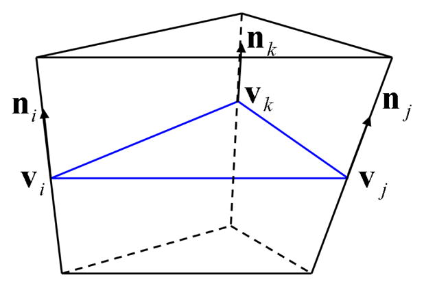
A prism D_ijk constructed based on the triangle [v_iv_jv_k].

$$B_{\mathit{ijk}}^n(b_1,b_2,b_3)=\frac{n!}{i!j!k!}{b}_1^i{b}_2^j{b}_3^k.$$

We approximate the molecular surface by the zero contour of F, denoted as S. In order to make S smooth, the degree of the Bezier basis n should be no less than 3. For simplicity, here we consider the case of n = 3. The control coefficients b_ijk(λ) should be properly defined such that S is continuous. In Figure 3 we show the relationship of the control coefficients and the points of the triangle when n = 3. Next we are going to discuss these coefficients are defined.

Fig. 3.

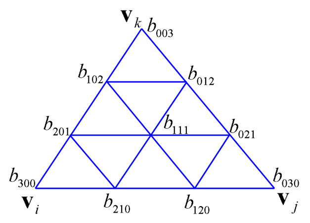
The control coefficients of the cubic Bezier basis of function F.

Since S passes through the vertices v_i, v_j, v_k, we define

$$b_{300}=b_{030}=b_{003}=\lambda .$$ (4)

Next we are going to define the coefficients on the edges of the triangle in Figure 3. To obtain C¹ continuity at v_i, we require that the directional derivatives of F at v_i in the direction of b₂ and b₃ are equal to ∇F · (v_j − v_i) and ∇F · (v_k − v_i), respectively. Noticing that F has the form of (3) and (b₁, b₂, b₃) = (1, 0, 0) at v_i, one can derive that $b_{210}-b_{300}=\frac{1}{3}\nabla F(v_i)·({\mathbf{v}}_j(\lambda )-{\mathbf{v}}_i(\lambda ))$, where ∇F(v_i) = n_i. Therefore

$$b_{210}=\lambda +\frac{1}{3}{\mathbf{n}}_i·({\mathbf{v}}_j(\lambda )-{\mathbf{v}}_i(\lambda )).$$ (5)

b₁₂₀, b₂₀₁, b₁₀₂, b₀₂₁, b₀₁₂ are defined similarly.

To obtain the C¹ continuity at the midpoints of the edges of , we define b₁₁₁ by using the side-vertex scheme [35]:

$$b_{111}=w_1{b}_{111}^{(1)}+w_2{b}_{111}^{(2)}+w_3{b}_{111}^{(3)},$$ (6)

where

$$w_i=\frac{b_j^2{b}_k^2}{b_2^2{b}_3^2+b_1^2{b}_3^2+b_1^2{b}_2^2},i=1,2,3,i\ne j\ne k.$$

Next we are going to define $b_{111}^{(1)},b_{111}^{(2)}$ and $b_{111}^{(3)}$. In Appendix V-A we prove that our scheme of defining this three coefficients can guarantee the C¹ continuity at the midpoints of the edges v_jv_k, v_iv_k and v_iv_j. Consider the edge v_iv_j. Recall that any point p = (x, y, z) in D_ijk can be represented by

$${(x,y,z)}^{\text{T}}=b_1{\mathbf{v}}_i(\lambda )+b_2{\mathbf{v}}_j(\lambda )+b_3{\mathbf{v}}_k(\lambda ).$$ (7)

Therefore differentiating both sides of (7) with respect to x, y and z, respectively, yields

$$I_3=\left(\begin{array}{ccc}\frac{\partial b_1}{\partial x}& \frac{\partial b_2}{\partial x}& \frac{\partial \lambda }{\partial x}\\ \frac{\partial b_1}{\partial y}& \frac{\partial b_2}{\partial y}& \frac{\partial \lambda }{\partial y}\\ \frac{\partial b_1}{\partial z}& \frac{\partial b_2}{\partial x}& \frac{\partial \lambda }{\partial z}\end{array}\right)\left(\begin{array}{c}{({\mathbf{v}}_i(\lambda )-{\mathbf{v}}_k(\lambda ))}^{\text{T}}\\ {({\mathbf{v}}_j(\lambda )-{\mathbf{v}}_k(\lambda ))}^{\text{T}}\\ {(b_1{\mathbf{n}}_i+b_2{\mathbf{n}}_j+b_3{\mathbf{n}}_k)}^{\text{T}}\end{array}\right),$$ (8)

where I₃ is a 3 × 3 unit matrix. Denote

$$M:=\left(\begin{array}{c}{({\mathbf{v}}_i(\lambda )-{\mathbf{v}}_k(\lambda ))}^{\text{T}}\\ {({\mathbf{v}}_j(\lambda )-{\mathbf{v}}_k(\lambda ))}^{\text{T}}\\ {(b_1{\mathbf{n}}_i+b_2{\mathbf{n}}_j+b_3{\mathbf{n}}_k)}^{\text{T}}\end{array}\right),$$ (9)

and let A = v_i(λ) − v_k(λ), B = v_j(λ) − v_k(λ) and C = b₁n_i +b₂n_j +b₃n_k, then M = (A B C)^T. From (8) we have

$$\left(\begin{array}{ccc}\frac{\partial b_1}{\partial x}& \frac{\partial b_2}{\partial x}& \frac{\partial \lambda }{\partial x}\\ \frac{\partial b_1}{\partial y}& \frac{\partial b_2}{\partial y}& \frac{\partial \lambda }{\partial y}\\ \frac{\partial b_1}{\partial z}& \frac{\partial b_2}{\partial z}& \frac{\partial \lambda }{\partial z}\end{array}\right)=M^{-1}=\frac{1}{det(M)}(B\times C,C\times A,A\times B).$$ (10)

According to (3), at the midpoint of v_iv_j, $(b_1,b_2,b_3)=(\frac{1}{2},\frac{1}{2},0)$, we have

$$\left(\begin{array}{c}\frac{\partial F}{\partial b_1}\\ \frac{\partial F}{\partial b_2}\\ \frac{\partial F}{\partial \lambda }\end{array}\right)=\left(\begin{array}{c}{({\mathbf{v}}_i(\lambda )-{\mathbf{v}}_k(\lambda ))}^{\text{T}}\\ {({\mathbf{v}}_j(\lambda )-{\mathbf{v}}_k(\lambda ))}^{\text{T}}\\ {({\mathbf{n}}_i+{\mathbf{n}}_j)}^{\text{T}}/2\end{array}\right)\left(\frac{{\mathbf{n}}_i+{\mathbf{n}}_j}{4}\right)+\left(\begin{array}{c}\frac{3}{2}(b_{210}-b_{111})\\ \frac{3}{2}(b_{120}-b_{111})\\ \frac{1}{2}\end{array}\right).$$

By (6), at $(b_1,b_2,b_3)=(\frac{1}{2},\frac{1}{2},0)$ we have $b_{111}=b_{111}^{(3)}$. Therefore the gradient at ( $\frac{1}{2},\frac{1}{2}$, 0) is

$$\begin{array}{l}\nabla F=M^{-1}{(\frac{\partial F}{\partial b_1},\frac{\partial F}{\partial b_2},\frac{\partial F}{\partial \lambda })}^{\text{T}}\\ =\frac{{\mathbf{n}}_i+{\mathbf{n}}_j}{4}+\frac{1}{2det(M)}[3(b_{210}-b_{111}^{(3)})B\times C+3(b_{120}-b_{111}^{(3)})C\times A+A\times B]\end{array}$$ (11)

Define vectors

$$\begin{array}{l}{\mathbf{d}}_1(\lambda )={\mathbf{v}}_j(\lambda )-{\mathbf{v}}_i(\lambda )=B-A,\\ {\mathbf{d}}_2(b_1,b_2,b_3)=b_1{\mathbf{n}}_i+b_2{\mathbf{n}}_j+b_3{\mathbf{n}}_k=C,\\ {\mathbf{d}}_3(b_1,b_2,b_3,\lambda )={\mathbf{d}}_1\times {\mathbf{d}}_2=B\times C+C\times A.\end{array}$$ (12)

Let

$$\mathbf{c}=C(\frac{1}{2},\frac{1}{2},0),$$ (13)

$${\mathbf{d}}_3(\lambda )={\mathbf{d}}_3(\frac{1}{2},\frac{1}{2},0,\lambda )=B\times \mathbf{c}+\mathbf{c}\times A.$$ (14)

Let $\nabla F=\nabla F(\frac{1}{2},\frac{1}{2},0)$. In order to have C¹ continuity at ( $\frac{1}{2},\frac{1}{2}$, 0), we should have ∇F · d₃(λ) = 0. Therefore, by (11) and (14), we have

$$b_{111}^{(3)}=\frac{{\mathbf{d}}_3{(\lambda )}^{\text{T}}(3b_{210}B\times \mathbf{c}+3b_{120}\mathbf{c}\times A+A\times B)}{3{\left|\right|{\mathbf{d}}_3(\lambda )\left|\right|}^2}.$$ (15)

Similarly, we may define $b_{111}^{(1)}$ and $b_{111}^{(2)}$.

Now the function F(b₁, b₂, b₃, λ) is well defined. The next step is to extract the zero level set S. Given the barycentric coordinates (b₁, b₂, b₃) of a point in the triangle [v_iv_jv_k], we find the corresponding λ by solving the equation F(b₁, b₂, b₃, λ) = 0 for λ and this could be done by the Newton’s method. Then we may get the corresponding point on S as

$${(x,y,z)}^{\text{T}}=b_1{\mathbf{v}}_i(\lambda )+b_2{\mathbf{v}}_j(\lambda )+b_3{\mathbf{v}}_k(\lambda ).$$ (16)

D. Smoothness

Theorem 2.1

The ASMS S is C¹ at the vertices of and the midpoints of the edges of .

Theorem 2.2

S is C¹ everywhere if every edge v_iv_j of satisfies n_i·(v_i − v_j) = n_j·(v_j − v_i).

Theorem 2.3

S is C¹ everywhere if the unit normals at the vertices of are the same.

Proofs of the theorems are shown in the Appendix.

E. Parametrization and quadrature

In this section, we would like to show how the ASMS is applied to the computation of (2). Since we use the ASMS to represent the molecular surface, now Γ = S. Let $f=\frac{(\mathbf{r}-{\mathbf{x}}_i)·\mathbf{n}(\mathbf{r})}{\mid \mathbf{r}-{\mathbf{x}}_i{\mid }^4}$. We decompose the entire surface S into patches {S_j} with S_j being the AMSM generated over triangle j, then we have

$${\int }_{S}f(\mathbf{x})dS=\sum _j{\int }_{S_j}f(\mathbf{x})dS.$$ (17)

For any point x = (x, y, z) on S_j, by the inverse map of (16), one can uniquely map x to a point in triangle j and get its baricentric coordinates (b₁, b₂, b₃) with b₃ = 1 − b₁ − b₂. Therefore, x, y, z can be represented in terms of (b₁, b₂):

$$x=x(b_1,b_2),y=y(b_1,b_2),z=z(b_1,b_2)$$

Replacing (x, y, z) with (b₁, b₁, b₃) in (17) and letting

$$g(b_1,b_2)=f(x(b_1,b_2),y(b_1,b_2),z(b_1,b_2)),$$

we get

$${\int }_{S_j}f(\mathbf{x})dS={\int }_{{\sigma }_j}g(b_1,b_2)\sqrt{EG-F^2}{db}_1{db}_2,$$ (18)

where

$$\begin{array}{l}E={(\frac{\partial x}{\partial b_1})}^2+{(\frac{\partial y}{\partial b_1})}^2+{(\frac{\partial z}{\partial b_1})}^2,\\ F=\frac{\partial x}{\partial b_1}\frac{\partial x}{\partial b_2}+\frac{\partial y}{\partial b_1}\frac{\partial y}{\partial b_2}+\frac{\partial z}{\partial b_1}\frac{\partial z}{\partial b_2},\\ G={(\frac{\partial x}{\partial b_2})}^2+{(\frac{\partial y}{\partial b_2})}^2+{(\frac{\partial z}{\partial b_2})}^2.\end{array}$$

We then apply the Gaussian quadrature to (18):

$${\int }_{{\sigma }_i}g(b_1,b_2)\sqrt{EG-F^2}{db}_1{db}_2\approx \sum _{k=1}^n{W}_{k}g(b_1^k,b_2^k)\sqrt{EG-F^2}{\mid }_{b_1^k,b_2^k},$$ (19)

where ( $b_1^k,b_2^k,b_3^k$) and W_k are the Gaussian integration nodes and weights on the triangles.

III. Error of the ASMS model

In order to show the error of S to the true surface S₀, we do a test on some typical surfaces (Table I) S₀:= {(x, y, z): z = f(x, y), (x, y) ∈ [0, 1]²} which are considered as the true surfaces. We generate a triangulation mesh over the true surface with the maximum edge length h being 0.1. Based on the mesh, we construct the ASMS model S. The error of S to S₀ is defined as $max\frac{\left|\right|\mathbf{p}-\mathbf{q}\left|\right|}{\left|\right|\mathbf{q}\left|\right|}$, where p ∈ S, q ∈ S₀, and p and q have the same (b₁, b₂, b₃) coordinates but different λ. We sample (p, q) on the surfaces and compute the maximum relative error. For the point pair p(b₁, b₂, b₃, λ_p) and q(b₁, b₂, b₃, λ_q) defined above, we prove that their Euclidean distance is bounded by the difference of their λ coordinates.

TABLE I.

Relative error and Convergence

Function (x, y) ∈ [0, 1]2	$max\left\{\frac{\left|\right|\mathbf{p}-\mathbf{q}\left|\right|}{\left|\right|\mathbf{q}\left|\right|}\right\}$	C
z = 0	0	0
z = x2 + y2	2.450030e-05	1.010636e-2
z = x3 + y3	1.063699e-04	2.610113e-2
$z=e^{-\frac{1}{4}[{(x-0.5)}^2+{(y-0.5)}^2]}$	5.286856e-07	6.288604e-5
$z=1.25+\frac{cos(5.4y)}{6+6{(3x-1)}^2}$	2.555683e-04	4.58608e-2
z = tanh(9y − 9x)	1.196519e-02	1.896754e-1
$z=\sqrt{1-x^2-y^2}$	8.614969e-05	1.744051e-1 (h4)
$z={[{(2-\sqrt{1-y^2})}^2-x^2]}^{1/2}$	1.418242e-05	1.748754e-02

Lemma 3.1

The error of the approximation point p to the true point q is bounded by |λ_p − λ_q|.

Proof

$$\begin{array}{l}\left|\right|\mathbf{p}-\mathbf{q}\left|\right|\le b_1\left|\right|{\mathbf{v}}_i({\lambda }_p)-{\mathbf{v}}_i({\lambda }_q)\left|\right|+b_2\left|\right|{\mathbf{v}}_j({\lambda }_q)-{\mathbf{v}}_j({\lambda }_q)\left|\right|+b_3\left|\right|{\mathbf{v}}_k({\lambda }_p)-{\mathbf{v}}_k({\lambda }_q)\left|\right|\\ \le \mid {\lambda }_p-{\lambda }_q\mid (b_1|\left|{\mathbf{n}}_i\right||+b_2|\left|{\mathbf{n}}_j\right||+b_3|\left|{\mathbf{n}}_k\right||)\\ =\mid {\lambda }_p-{\lambda }_q\mid \end{array}$$

To study the rate of converges of S to S₀, we gradually refine the initial mesh. Since the error is bounded by |λ_p − λ_q|, we compute the ratio of the maximum difference of λ_p and λ_q to h, h², h³, and so forth. As h decreases, we check if the ratio converges or not, which allows us to know the highest rate of convergence of S to S₀. For most of the test functions in Table I, we observe that S converges to S₀ as fast as O(h³). We also observe that for the case $z=\sqrt{1-x^2-y^2}$, the rate of convergence reaches O(h⁴). We show the limit of the ratio $\frac{\mid \lambda -{\lambda }^{\prime }\mid }{h^3}$ as h ↓ 0, denoted as C, in Table I. Hence we draw the following claim:

Claim

Let h be the maximum side length of triangulation mesh , p be the point on the ASMS, q be the corresponding point on the true surface, then p converges to q at the rate of O(h³). i.e. There exists a constant C such that ||p − q|| ≤ Ch³.

We generated the ASMS for the real proteins based on different size of meshes (Figure 4) and show the error of the ASMS to the SES of three proteins: 1GCQ (843 atoms), 1ML0 (1051 atoms), and 1KKL (1276 atoms) in Table II. Here the SES is modeled as a level set of the summation of fast decaying Gaussian functions. The ASMS is generated from the triangulation of the SES at different resolution. The number of triangles of the initial meshes are listed in Table II. The error ε_max is defined as the one-way Hausdorff distance from the ASMS to the SES: ${\epsilon }_{\mathit{max}}=\underset{\mathbf{p}\in \text{ASMS}}{max}\underset{\mathbf{q}\in \text{SES}}{min}\left|\right|\mathbf{p}-\mathbf{q}\left|\right|$. As we see in the table, the errors are small and decrease rapidly as the initial triangulation becomes dense.

Fig. 4.

The top row is the triangulation of the SES of protein 1ML0 with different number of triangles. The bottom row is the ASMS generated from the above corresponding triangulation.

TABLE II.

Error of ASMS to the SES

1GCQ		1ML0		1KKL
No. of Δs	εmax	No. of Δs	εmax	No. of Δs	εmax
16,312	0.266069	18,400	0.233949	19,968	0.260418
32,624	0.142149	36,864	0.142380	39,544	0.134689
65,456	0.082550	73,736	0.083895	79,096	0.085855

IV. Application to the biomolecular energetic computation

We apply the ASMS model to the GB electrostatic solvation energy computations of the example proteins 1PPE (436 atoms), 1HIA (693 atoms), 1CGI (852 atoms), 7CEI (1912 atoms), 1F15 (7704 atoms), and 1KXP (11859 atoms). The ASMS models S for the proteins are generated based on the initial mesh with different number of triangles (Table III). We show the ASMS of the example molecules generated from the decimated triangulations in Figure 5 and Figure 6. As a comparison, we compute the polarization energy G_pol for both the ASMS and the piecewise linear (PL) surfaces and show the energy results and the timing in Table III. For all the computations, a 4-point Gaussian quadrature rule over a triangle [36] is used for the numerical integration in (19) when computing the Born radii. The running time contains the time cost of computing the integration nodes over the surfaces, computing the Born radii, and evaluating G_pol. If we consider the energy computed from the dense mesh as accurate, as we see from the table, the G_pol computed from the coarse PL model has a large error, however for the coarse ASMS model, it is very close to the dense mesh result but with less time. On the other hand, to get a energy result of the same accuracy, fewer number of triangles are needed for the ASMS model than the PL model. For example, for the protein 1CGI, the G_pol computed from the ASMS with 3674 triangles is −1394.227 kcal/mol. However to get a similar result, 8712 triangles are needed for the piecewise linear model. Therefore the ASMS model is much more efficient in the energetic computation than trivial piecewise linear models.

TABLE III.

ELECTROSTATIC SOLVATION ENERGY AND TIMING

Protein ID	No. of Triangles	Gpol (kcal/mol)		Timing (s)
		PL	AS	PL	AS
1PPE	24244	−835.5639	−825.3252	17.27	18.26
	6004	−852.7130	−828.2158	5.09	5.39
	2748	−933.9562	−845.5085	2.74	3.27
1HIA	27480	−1361.2266	−1340.6384	30.23	31.18
	7770	−1389.0175	−1347.8067	9.43	9.93
	3510	−1571.8908	−1388.4665	5.21	5.21
1CGI	29108	−1371.7419	−1343.1496	39.64	40.31
	8712	−1399.1948	−1346.2230	12.94	12.64
	3674	−1678.4447	−1394.2270	7.40	6.11
7CEI	54544	−3758.7928	−3711.3626	29.04	29.96
	17044	−3771.7803	−3753.3377	10.03	9.89
	5324	−3876.7333	−3826.1959	4.11	4.08
1F51	87516	−11656.0327	−11411.9689	123.55	121.52
	33660	−11691.4450	−11622.8886	51.95	52.56
	8290	−12527.8362	−11721.4931	21.01	21.55
1KXP	402812	−13258.0206	−13121.3053	975.08	977.96
	134272	−13325.0423	−13264.7272	340.16	346.31
	94352	−14669.1209	−14071.9965	246.68	244.33

Fig. 5.

Molecular models of a protein(1HIA). (a) is The atomic model. (b) is the initial dense mesh of the SES (27480 triangles). (c) is the decimated mesh of the SES model (7770 triangles). (d) is the ASMS (7770 patches) generated from (c).

Fig. 6.

The top row are the models of 1CGI and the bottom row are the models of 1PPE. (a) and (d) are the atomic structures of the proteins. (b) and (e) are the decimated triangular meshes of the proteins with 8712 triangles and 6004 triangles, respectively. (c) and (f) are the ASMS models generated from (b) and (e), respectively.

V. Conclusions

We have introduced a method to generate a model for the molecular surface. Like the other molecular surface models, this ASMS model is smooth and close to the SES as long as the initial triangulation is based on the SES. In addition, it has dual implicit and parametric representations. The implicit representation enables us to flexibly vary the surface by selecting different level sets, while the parametric representation allows us easily apply the ASMS to the numerical computations, such as the numerical integrations involved in the finite element method or the boundary element method. Moreover, unlike the other piecewise linear models, the ASMS surface is of higher degree, therefore, to get the same accuracy, fewer number of triangles (roughly one-third of the PL model) are needed for the ASMS when it is applied to the numerical integrations. For many large system problems, for example the atomistic molecular dynamics simulations, efficient computation is the most concerning issue, hence he ASMS is very suitable to be used in this kind of problems. We should mention that, while not detailed in this paper, the algorithm of Section II-C can, by repeated evocation, yield a hierarchical multiresolution spline model of the molecular surface. In the future research we could extend this algebraic patch model to the electrostatic solvation forces calculation which is crucial in the molecular dynamics simulations. Fast and accurate numerical integration is also one of the main tasks of the force calculation and is more challenging because the integration domain contains not only the surface but also a skin layer over each atom.

Appendix

A. Proof of Theorem 2.1

Proof

It is obvious that S is C¹ at the vertices. For the continuity at the midpoints of edges, let us consider the edge v_iv_j in triangle [v_iv_jv_k]. On the edge v_iv_j, b₃ = 0. So we may let b₂ = t and b₁ = 1 − t. Then matrix M can be written as

$$M(t)=\left(\begin{array}{c}{({\mathbf{v}}_i(\lambda )-{\mathbf{v}}_k(\lambda ))}^{\text{T}}\\ {({\mathbf{v}}_j(\lambda )-{\mathbf{v}}_k(\lambda ))}^{\text{T}}\\ {({\mathbf{n}}_i+t({\mathbf{n}}_j-{\mathbf{n}}_i))}^{\text{T}}\end{array}\right),$$

and

$$M^{-1}=\frac{1}{det(M)}(B\times C,C\times A,A\times B),$$

where A = v_i(λ) − v_k(λ), B = v_j(λ) − v_k(λ) and C(t) = n_i + t(n_j − n_i). Therefore on the edge v_iv_j,

$$\left(\begin{array}{c}\frac{\partial F}{\partial b_1}\\ \frac{\partial F}{\partial b_2}\\ \frac{\partial F}{\partial \lambda }\end{array}\right)=\left(\begin{array}{c}{A}^{\text{T}}\\ B^{\text{T}}\\ C^{\text{T}}\end{array}\right)({\mathbf{n}}_i{(1-t)}^2+{\mathbf{n}}_j{t}^2)+\left(\begin{array}{c}3(b_{210}-b_{111})\\ 3(b_{120}-b_{111})\\ 1\end{array}\right)2t(1-t).$$

The gradient of F on the edge v_iv_j can be written as

$$\begin{array}{l}\nabla F={\mathbf{n}}_i{(1-t)}^2+{\mathbf{n}}_j{t}^2+M^{-1}\left(\begin{array}{c}3(b_{210}-b_{111})\\ 3(b_{120}-b_{111})\\ 1\end{array}\right)2t(1-t)\\ ={\mathbf{n}}_i{(1-t)}^2+{\mathbf{n}}_j{t}^2+\frac{2t(1-t)}{det(M)(t)}[3(B\times C(t))(b_{210}-b_{111})\\ +3(C(t)\times A)(b_{120}-b_{111})+A\times B].\end{array}$$ (20)

When $t=\frac{1}{2},C(\frac{1}{2})=\mathbf{c}$, therefore

$$B\times C(t)+C(t)\times A={\mathbf{d}}_3(\lambda ).$$

Consider the function inside the square bracket of (20) and denote it as F₁. Then

$$F_1=3(B\times \mathbf{c})b_{210}+3(\mathbf{c}\times A)(b_{120}+A\times B-3(B\times \mathbf{c}+\mathbf{c}\times A)b_{111}.$$ (21)

Since on the edge v_iv_j, $b_{111}=b_{111}^{(3)}$, substituting (15) into (21), we get F₁ is 0. Therefore, at the midpoint

$$\nabla F=({\mathbf{n}}_i+{\mathbf{n}}_j)/4.$$ (22)

So S is C¹ continuous at the midpoints of the edges.

B. Proof of Theorem 2.2

Proof

It is obvious that S is C¹ within the triangles. By Theorem 2.1 we have already known that S is C¹ at the vertices and the midpoints of the edges. Here we only need to show S is C¹ at any points of the edges, let us consider the the edge v_iv_j in the triangle [v_iv_jv_k].

Under the condition n_i · (v_i − v_j) = n_j · (v_j − v_i), we have b₁₂₀ = b₂₁₀, so (20) is written as

$$\nabla F={\mathbf{n}}_i{(1-t)}^2+{\mathbf{n}}_j{t}^2+\frac{2t(1-t)}{det(M(t))}[3(b_{210}-b_{111})(B-A)\times C+A\times B].$$ (23)

Similar as (12), we define

$${\mathbf{d}}_3(t,\lambda )=(B-A)\times C(t).$$ (24)

By (15) together with the facts that b₁₂₀ = b₂₁₀ and $b_{111}=b_{111}^{(3)}$ on edge v_iv_j, we have

$$b_{210}-b_{111}=-\frac{{\mathbf{d}}_3^{\text{T}}(\lambda )(A\times B)}{3{\left|\right|{\mathbf{d}}_3(\lambda )\left|\right|}^2},$$ (25)

where d₃(λ) is defined in (14). Plug (24) and (25) in (23), we get

$$\begin{array}{l}\nabla F={\mathbf{n}}_i{(1-t)}^2+{\mathbf{n}}_j{t}^2\\ +\frac{2t(1-t)}{{\left|\right|{\mathbf{d}}_3(\lambda )\left|\right|}^2}\left[\frac{{\left|\right|{\mathbf{d}}_3(\lambda )\left|\right|}^{2}A\times B-{\mathbf{d}}_3(t,\lambda ){\mathbf{d}}_3^{\text{T}}(\lambda )A\times B}{det(M(t))}\right].\end{array}$$ (26)

Consider the function inside the square bracket of (26) and denote it as F₂. Our goal is to show that F₂ = 0. Since we have already known that when $t=\frac{1}{2}$, F₂ = 0, this prompts us to compute the derivative of F₂ with respect to t and see if the derivative is 0. We observe that both the numerator of the denominator of F₂ are linear in terms of t, so F₂ is of the form $\frac{at+b}{ct+d}$ with

$$\begin{array}{l}a=({\mathbf{n}}_j-{\mathbf{n}}_i)\times (B-A){\mathbf{d}}_3^{\text{T}}(\lambda )A\times B,\\ b={\left|\right|{\mathbf{d}}_3(\lambda )\left|\right|}^{2}A\times B+{\mathbf{n}}_i\times (B-A){\mathbf{d}}_3^{\text{T}}(\lambda )A\times B,\\ c={({\mathbf{n}}_j-{\mathbf{n}}_i)}^{\text{T}}(A\times B),\\ d={\mathbf{n}}_i^{\text{T}}(A\times B).\end{array}$$

In order to show $\frac{\partial F_2}{\partial t}=0$, which is equivalent to show N:= ad − bc = 0, we compute

$$\begin{array}{l}N=[{\mathbf{n}}_j\times (B-A){\mathbf{d}}_3^{\text{T}}A\times B]{\mathbf{n}}_i^{\text{T}}(A\times B)\\ -({\left|\right|{\mathbf{d}}_3(\lambda )\left|\right|}^{2}A\times B)({\mathbf{n}}_j-{\mathbf{n}}_i)\times (B-A)\\ -[{\mathbf{n}}_i\times (B-A){\mathbf{d}}_3^{\text{T}}A\times B]{\mathbf{n}}_j^{\text{T}}(A\times B).\end{array}$$ (27)

Under the condition n_i · (v_i − v_j) = n_j · (v_j − v_i), we have (B − A)^Tc = (v_j(λ) − v_i(λ))^Tc = 0, where $\mathbf{c}=C(\frac{1}{2},\frac{1}{2},0)$. Therefore

$${\left|\right|{\mathbf{d}}_3(\lambda )\left|\right|}^2=((B-A)\times \mathbf{c})·((B-A)\times \mathbf{c})={\left|\right|{\mathbf{v}}_j(\lambda )-{\mathbf{v}}_i(\lambda )\left|\right|}^2{\left|\right|\mathbf{c}\left|\right|}^2,$$ (28)

and

$$\begin{array}{l}{\mathbf{d}}_3^{\text{T}}(\lambda )A\times B={\mathbf{d}}_3^{\text{T}}(\lambda )A\times (B-A)\\ =((B-A)\times \mathbf{c})·(A\times (B-A))=-{\mathbf{c}}^{\text{T}}A{\left|\right|{\mathbf{v}}_j(\lambda )-{\mathbf{v}}_i(\lambda )\left|\right|}^2.\end{array}$$ (29)

Plug (28) and (29) into (27) and divide both sides by ||v_j(λ) − v_i(λ)||², we get

$$\begin{array}{l}{F}_3:=\frac{N}{{\left|\right|({\mathbf{v}}_j-{\mathbf{v}}_i)(\lambda )\left|\right|}^2}\\ =-{\mathbf{n}}_j\times (B-A){\mathbf{c}}^{\text{T}}A{\mathbf{n}}_i^{\text{T}}(A\times B)-{\left|\right|\mathbf{c}\left|\right|}^{2}A\times B{({\mathbf{n}}_j-{\mathbf{n}}_i)}^{\text{T}}A\times B\\ +({\mathbf{n}}_i\times (B-A){\mathbf{c}}^{\text{T}}A){\mathbf{n}}_j^{\text{T}}(A\times B)\\ =[({\mathbf{c}}^{\text{T}}A{\mathbf{n}}_i-{\left|\right|\mathbf{c}\left|\right|}^{2}A)\times (B-A)]{\mathbf{n}}_j^{\text{T}}(A\times B)\\ +[({\left|\right|\mathbf{c}\left|\right|}^{2}A-{\mathbf{c}}^{\text{T}}A{\mathbf{n}}_j)\times (B-A)]{\mathbf{n}}_i^{\text{T}}(A\times B).\end{array}$$ (30)

If n_i = n_j, (30) is 0. Now let us assume n_i ≠ n_j. Recall that $\mathbf{c}=\frac{1}{2}({\mathbf{n}}_i+{\mathbf{n}}_j)$. we define another vector $\mathbf{e}=\frac{1}{2}({\mathbf{n}}_i-{\mathbf{n}}_j)$ and let D = B − A. Then c is orthogonal to e and D:

$${\mathbf{c}}^{\text{T}}\mathbf{e}=0,{\mathbf{c}}^{\text{T}}D=0.$$ (31)

Furthermore

$$\mathbf{c}\times (D\times \mathbf{e})=0.$$ (32)

By the definition of c and e,

$${\mathbf{n}}_i=\mathbf{c}+\mathbf{e},{\mathbf{n}}_j=\mathbf{c}-\mathbf{e}.$$ (33)

Substitute (33) into (30) and replace A × B with A × D, we get

$$\begin{array}{l}{F}_3=[{\mathbf{c}}^{T}A(\mathbf{c}+\mathbf{e})-{\left|\right|\mathbf{c}\left|\right|}^{2}A]\times D{(\mathbf{c}-\mathbf{e})}^{\text{T}}(A\times D)\\ +[{\left|\right|\mathbf{c}\left|\right|}^{2}A-{\mathbf{c}}^{\text{T}}A(\mathbf{c}-\mathbf{e})]\times D{(\mathbf{c}+\mathbf{e})}^{\text{T}}(A\times D)\\ =2{\mathbf{c}}^{\text{T}}A(\mathbf{e}\times D){\mathbf{c}}^{\text{T}}(A\times D)\\ -2[{\mathbf{c}}^{\text{T}}A\mathbf{c}-{\left|\right|\mathbf{c}\left|\right|}^{2}A]\times D{\mathbf{e}}^{\text{T}}(A\times D).\end{array}$$ (34)

If e and D are linearly dependent, then e × D = 0, moreover e(A × D) = 0, which yields F₃ = 0. Otherwise, we introduce a new matrix

$$M=\left(\begin{array}{c}{D}^{\text{T}}\\ {\mathbf{c}}^{\text{T}}\\ {\mathbf{e}}^{\text{T}}\end{array}\right).$$

Since c, e, and D are linearly independent, M is nonsingular. So F₃ (a vector) is equal to

$$\begin{array}{l}2M^{-1}\left(\begin{array}{c}{D}^{\text{T}}\\ {\mathbf{c}}^{\text{T}}\\ {\mathbf{e}}^{\text{T}}\end{array}\right)({\mathbf{c}}^{\text{T}}A(\mathbf{e}\times D){\mathbf{c}}^{\text{T}}(A\times D)-[{\mathbf{c}}^{\text{T}}A\mathbf{c}-{\left|\right|\mathbf{c}\left|\right|}^{2}A]\times D{\mathbf{e}}^{\text{T}}(A\times D))\\ =-2M^{-1}\left(\begin{array}{c}0\\ (-{\mathbf{c}}^{\text{T}}A{\mathbf{c}}^{\text{T}}(\mathbf{e}\times D)-{\left|\right|\mathbf{c}\left|\right|}^2{\mathbf{e}}^{\text{T}}(A\times D)){\mathbf{c}}^{\text{T}}(A\times D)\\ ({\mathbf{c}}^{\text{T}}A{\mathbf{e}}^{\text{T}}(\mathbf{c}\times D)-{\left|\right|\mathbf{c}\left|\right|}^2{\mathbf{e}}^{\text{T}}(A\times D)){\mathbf{e}}^{\text{T}}(A\times D)\end{array}\right)\\ =-2M^{-1}\left(\begin{array}{c}0\\ ({\mathbf{c}}^{\text{T}}A{\mathbf{c}}^{\text{T}}(D\times \mathbf{e})-{\left|\right|\mathbf{c}\left|\right|}^2{A}^{\text{T}}(D\times \mathbf{e})){\mathbf{c}}^{\text{T}}(A\times D)\\ ({\mathbf{c}}^{\text{T}}A{\mathbf{c}}^{\text{T}}(D\times \mathbf{e})-{\left|\right|\mathbf{c}\left|\right|}^2{A}^{\text{T}}(D\times \mathbf{e})){\mathbf{e}}^{\text{T}}(A\times D)\end{array}\right)\\ =-2[{\mathbf{c}}^{\text{T}}A{\mathbf{c}}^{\text{T}}(D\times \mathbf{e})-{\left|\right|\mathbf{c}\left|\right|}^2{A}^{\text{T}}(D\times \mathbf{e})]M^{-1}\left(\begin{array}{c}0\\ {\mathbf{c}}^{\text{T}}(A\times D)\\ {\mathbf{e}}^{\text{T}}(A\times D)\end{array}\right).\end{array}$$

By the Lagrange’s formula:

$${\mathbf{c}}^{\text{T}}A{\mathbf{c}}^{\text{T}}(D\times \mathbf{e})-{\left|\right|\mathbf{c}\left|\right|}^2{A}^{\text{T}}(D\times \mathbf{e})=(\mathbf{c}\times A)·(\mathbf{c}\times (D\times \mathbf{e})),$$ (35)

and (32), (35) is zero and thus F₃ = 0. So far we have proved that F₂ is independent of t. Meanwhile in the proof of Theorem 2.1, we know that F₂ = 0 at $t=\frac{1}{2}$. Hence F₂ = 0 for all t and therefore on the edge v_iv_j, ∇F is

$$\nabla F={\mathbf{n}}_i{(1-t)}^2+{\mathbf{n}}_j{t}^2.$$

So S is C¹ on the edges.

C. Proof of Theorem 2.3

Proof

As same as the proof of Theorem 2.2, we only need to show that S is C¹ on the edge v_iv_j. In the proof of Theorem 2.1, we have already derived the gradient function on the edge v_iv_j (20):

$$\begin{array}{c}\nabla F={\mathbf{n}}_i{(1-t)}^2+{\mathbf{n}}_j{t}^2+\frac{2t(1-t)}{det(M)(t)}[3(B\times C(t))(b_{210}-b_{111})\\ +3(C(t)\times A)(b_{120}-b_{111})+A\times B].\end{array}$$

Let

$$F_4=\frac{1}{det(M)(t)}[3(B\times C(t))(b_{210}-b_{111})+3(C(t)\times A)(b_{120}-b_{111})+A\times B].$$ (36)

Following the same idea of the proof the Theorem 2.2, we compute $\frac{\partial F_4}{\partial t}$. The numerator of $\frac{\partial F_4}{\partial t}$ is

$$\begin{array}{l}[3(B\times C^{\prime }(t))(b_{210}-b_{111})+3(C^{\prime }(t)\times A)(b_{120}-b_{111})\\ +A\times B]det(M)-det{(M)}^{\prime }(t)[3(B\times C(t))(b_{210}-b_{111})\\ +3(C(t)\times A)(b_{120}-b_{111})+A\times B].\end{array}$$ (37)

Since

$$\begin{array}{l}{C}^{\prime }(t)={\mathbf{n}}_j-{\mathbf{n}}_i,\text{and}\\ det{(M)}^{\prime }(t)={({\mathbf{n}}_j-{\mathbf{n}}_i)}^{\text{T}}(A\times B),\end{array}$$

(37) is 0 when n_i = n_j. So F₄ is independent of t. By the proof of Theorem 2.1, F₄ = 0 at $t=\frac{1}{2}$. So F₄ = 0 for all t. So S is C¹ continuous.

References

- 1.Karplus Martin, Andrew McCammon J. Molecular dynamics simulations of biomolecules. Nature Structural Biology. 2002;9:646–652. doi: 10.1038/nsb0902-646. [DOI] [PubMed] [Google Scholar]
- 2.Srinivasan J, Cheatham TE, Cieplak P, Kollman PA, Case DA. Continuum solvent studies of the stability of dna, rna, and phosphoramidate-dna helices. J Am Chem Soc. 1998;120:9401–9409. [Google Scholar]
- 3.Kuhn B, Kollman PA. A ligand that is predicted to bind better to avidin than biotin: insights from computational fluorine scanning. J Am Chem Soc. 2000;122:3909–3916. [Google Scholar]
- 4.Nina M, Beglov D, Roux B. Atomic radii for continuum electrostatics calculations based on molecular dynamics free energy simulations. J Phys Chem B. 1997;101:5239–5248. [Google Scholar]
- 5.Roux B, Simonson T. Implicit solvent models. Biophysical Chemistry. 1999;78:1–20. doi: 10.1016/s0301-4622(98)00226-9. [DOI] [PubMed] [Google Scholar]
- 6.Schaefer M, Karplus M. A comprehensive analytical treatment of continuum electrostatics. J Phys Chem. 1996;100:1578–1599. [Google Scholar]
- 7.Baker N, Holst M, Wang F. Adaptive multilevel finite element solution of the poisson-boltzmann equation ii. refinement at solvent-accessible surfaces in biomolecular systems. J Comput Chem. 2000;21:1343–1352. [Google Scholar]
- 8.Madura JD, Briggs JM, Wade RC, Davis ME, Luty BA, Ilin A, Antosiewicz J, Gilson MK, Bagheri B, Scott LR, McCammon JA. Electrostatics and diffusion of molecules in solution: simulations with the university of houston brownian dynamics program. Computer Physics Communications. 1995;91:57–95. [Google Scholar]
- 9.Still WC, Tempczyk A, Hawley RC, Hendrickson T. Semianalytical treatment of solvation for molecular mechanics and dynamics. J Am Chem Soc. 1990;112:6127–6129. [Google Scholar]
- 10.Bashford D, Case DA. Generalized born models of macromolecular solvation effects. Annu Rev Phys Chem. 2000;51:129–152. doi: 10.1146/annurev.physchem.51.1.129. [DOI] [PubMed] [Google Scholar]
- 11.Lee MS, Feig M, Salsbury FR, Brooks CL. New analytic approximation to the standard molecular volume definition and its application to generalized born calculations. J Comput Chem. 2003;24:1348–1356. doi: 10.1002/jcc.10272. [DOI] [PubMed] [Google Scholar]
- 12.Ghosh A, Rapp CS, Friesner RA. Generalized born model based on a surface integral formulation. J Phys Chem B. 1998;102:10983–10990. [Google Scholar]
- 13.Bajaj C, Siddavanahalli V, Zhao W. Fast algorithms for molecular interface triangulation and solvation energy computations. 2007 ICES Technical Report TR-07-06. [Google Scholar]
- 14.Lee B, Richards FM. The interpretation of protein structure: estimation of static accessiblilty. J Mol Biol. 1971;55:379–400. doi: 10.1016/0022-2836(71)90324-x. [DOI] [PubMed] [Google Scholar]
- 15.Connolly ML. Analytical molecular surface calculation. J Appl Cryst. 1983;16:548–558. [Google Scholar]
- 16.Richards FM. Areas, volumes, packing, and protein structure. Annu Rev Biophys Bioeng. 1977;6:151–176. doi: 10.1146/annurev.bb.06.060177.001055. [DOI] [PubMed] [Google Scholar]
- 17.Grant JA, Pickup BT. A gaussian description of molecular shape. J Phys Chem. 1995;99:3503–3510. [Google Scholar]
- 18.Lee MS, Salsbury FR, Brooks CL. Novel generalized born methods. J Chemical Physics. 2002;116:10606–10614. [Google Scholar]
- 19.Bajaj C, Castrillon-Candas J, Siddavanahalli V, Xu Z. Compressed representations of macromolecular structures and properties. Structure. 2005;13:463–471. doi: 10.1016/j.str.2005.02.004. [DOI] [PubMed] [Google Scholar]
- 20.Bajaj C, Siddavanahalli V. Fast error-bounded surfaces and derivatives computation for volumetric particle data. 2006 ICES Technical Report TR-06-06. [Google Scholar]
- 21.Bajaj C, Lee H, Merkert R, Pascucci V. Nurbs based b-rep models from macromolecules and their properties. Proceedings of Fourth Symposium on Solid Modeling and Applications; 1997. pp. 217–228. [Google Scholar]
- 22.Edelsbrunner H. Deformable smooth surface design. Discrete Computational Geometry. 1999;21:87–115. [Google Scholar]
- 23.Cheng H, Shi X. Guaranteed quality triangulation of molecular skin surfaces. IEEE Visualization. 2004:481–488. [Google Scholar]
- 24.Cheng H, Shi X. Quality mesh generation for molecular skin surfaces using restricted union of balls. IEEE Visualization. 2005:51–58. [Google Scholar]
- 25.Dahmen W. Smooth piecewise quadratic surfaces. In: Lyche T, Schumaker L, editors. Mathematical methods in computer aided geometric design. Academic Press; Boston: 1989. pp. 181–193. [Google Scholar]
- 26.Guo B. PhD thesis. Cornell University; 1991. Modeling arbitrary smooth objects with algebraic surfaces. [Google Scholar]
- 27.Dahmen W, Thamm-Schaar TM. Cubicoids: modeling and visualization. Computer Aided Geometric Design. 1993;10:89–108. [Google Scholar]
- 28.Bajaj C, Chen J, Xu G. Modeling with cubic A-patches. ACM Transactions on Graphics. 1995;14:103–133. [Google Scholar]
- 29.Akkiraju N, Edelsbrunner H. Triangulating the surface of a molecule. Discrete Applied Mathematics. 1996;71:5–22. [Google Scholar]
- 30.Laug P, Borouchaki H. Molecular surface modeling and meshing. Engineering with Computers. 2002;18:199–210. [Google Scholar]
- 31.Zhang Y, Xu G, Bajaj C. Quality meshing of implicit solvation models of biomolecular structures. Computer Aided Geometric Design. 2006;23:510–530. doi: 10.1016/j.cagd.2006.01.008. [DOI] [PMC free article] [PubMed] [Google Scholar]
- 32.Bajaj C, Siddavanahalli V. An adaptive grid based method for computing molecular surfaces and properties. 2006 ICES Technical Report TR-06-57. [Google Scholar]
- 33.Bajaj C, Djeu P, Siddavanahalli V, Thane A. Texmol: Interactive visual exploration of large flexible multi-component molecular complexes. Proc. of the Annual IEEE Visualization Conference; 2004. pp. 243–250. [Google Scholar]
- 34.Bajaj C, Xu G, Holt R, Netravali A. Hierarchical multiresolution reconstruction of shell surfaces. Computer Aided Geometric Design. 2002;19:89–112. [Google Scholar]
- 35.Nielson G. The side-vertex method for interpolation in triangles. J Apprrox Theory. 1979;25:318–336. [Google Scholar]
- 36.Dunavant D. High degree efficient symmetrical gaussian quadrature rules for the triangle. International Journal for Numerical Methods in Engineering. 1985;21:1129–1148. [Google Scholar]