The Impact of Survey and Response Modes on Current Smoking Prevalence Estimates Using TUS-CPS: 1992-2003

Abstract

This study identified whether survey administration mode (telephone or in-person) and respondent type (self or proxy) result in discrepant prevalence of current smoking in the adult U.S. population, while controlling for key sociodemographic characteristics and longitudinal changes of smoking prevalence over the 11-year period from 1992-2003. We used a multiple logistic regression analysis with replicate weights to model the current smoking status logit as a function of a number of covariates. The final model included individual- and family-level sociodemographic characteristics, survey attributes, and multiple two-way interactions of survey mode and respondent type with other covariates. The respondent type is a significant predictor of current smoking prevalence and the magnitude of the difference depends on the age, sex, and education of the person whose smoking status is being reported. Furthermore, the survey mode has significant interactions with survey year, sex, and age. We conclude that using an overall unadjusted estimate of the current smoking prevalence may result in underestimating the current smoking rate when conducting proxy or telephone interviews especially for some sub-populations, such as young adults. We propose that estimates could be improved if more detailed information regarding the respondent type and survey administration mode characteristics were considered in addition to commonly used survey year and sociodemographic characteristics. This information is critical given that future surveillance is moving toward more complex designs. Thus, adjustment of estimates should be contemplated when comparing current smoking prevalence results within a given survey series with major changes in methodology over time and between different surveys using various modes and respondent types.

1 Introduction

Scientific knowledge about the health effects of smoking has increased greatly over the past decades. The first U.S. Surgeon General’s report on active tobacco use and associated health consequences was released in 1964, U.S. Department of Health, Education, and Welfare (1964). The most recent report was released in 2004, U.S. Department of Health and Human Services (2004). More than 440,000 deaths per year among adults in the United States are caused by tobacco use, Centers for Disease Control and Prevention (2002).

The National Health Interview Survey (NHIS) is commonly used as one of the standards for determining current smoking prevalence in the U.S. adult population. The research findings based on the NHIS data indicate that the percentage of current smokers in the U.S. has declined over the past four decades from 42.2% in 1965 to 20.8% in 2006, Centers for Disease Control & Prevention (2008). Another survey that is used to provide valid estimates of current smoking prevalence in the U.S. adult population is the Tobacco Supplement to the Current Population Survey (TUS-CPS). Although the TUS-CPS is conducted less frequently than the NHIS, it has a much larger sample size than the NHIS and thus, it allows for estimates of smoking prevalence with smaller standard errors for small groups and geographical regions, National Cancer Institute (2007a). These characteristics are why smoking prevalence estimates based on the TUS-CPS data are widely used in many tobacco research studies, National Cancer Institute (2007b, 2007c) and have been used as one standard for state estimates, see Biener et al. (2004).

In this paper we present a detailed analysis of TUS-CPS data in which our primary goal was to identify survey methodologic factors that highly influence smoking prevalence trend results. Numerous studies show that current smoking prevalence depends on demographic characteristics. For example, Shavers et al. (2005) assessed racial/ethnical differences in current smoking by occupation and industry based on the TUS-CPS for 1998-1999. They estimated that American Indians and Alaska Natives had the highest smoking prevalence, at 35.1%, whereas Asian and Pacific Islanders had the lowest rate, at 15.2%. These patterns were consistent with those of the NHIS, Centers for Disease Control and Prevention (2008). Fagan et al. (2007) investigated the sociodemographic factors associated with smoking among unemployed adults based on the TUS-CPS data for 1998-1999 and 2001-2002. In particular, the authors examined employment attributes in relationship to current and former smoking and successful quitting among unemployed adults. Green et al. (2007) used 2003 TUS-CPS data to examine the relationship between smoking behaviors of young adults and their education level, and concluded that education was an important predictor of current smoking prevalence and that young adults with a college education were half as likely to smoke as those without a college education. Pleis and Lethbridge-Çejku (2007) investigated specific chronic conditions such as smoking with respect to multiple sociodemographic characteristics, including education level. They concluded that adults with at least a bachelor’s degree were less likely to smoke than the other adults and they were more likely to have never smoked in their past. These results reinforce a common research finding that race/ethnicity, employment status, and education are important predictors of current smoking prevalence.

To identify the unique contributions of survey methodologic factors on smoking prevalence, we investigated whether and to what degree respondent type and survey administration mode affect current smoking prevalence estimates. Our basic assumption in conducting this analysis was that self-reports provide a valid assessment of current smoking. This assumption is supported by the results of a comparison of self-reported smoking prevalence to the biochemical measurement of serum cotinine concentration, which used data from the Third National Health and Examination Survey for 1988-1994, Caraballo et al., (2001). The authors conclude that the overall smoking estimates based on self-reports and the biochemical measurements are approximately the same. These findings also confirm a meta-analysis conducted by Patrick et al. (1994), which investigated 26 publications presenting 51 comparisons between self-reported smoking and biochemical measures of smoking. The authors concluded that in most of the studies, self-reports of smoking provided an accurate measure of smoking. Hence, self-reports can be used to obtain viable information regarding current smoking status.

Our first research goal was to investigate whether in addition to self-responses proxy-responses can be relied on to accurately estimate current smoking prevalence. Including proxy-respondents in a survey is highly beneficial because it reduces survey costs and increases response rates, but proxy-responses usually result in higher measurement error. We review some general results regarding self- and proxy-respondents and then discuss this topic with respect to smoking, specifically.

Sudman, Bradburn and Schwarz (1996, Chapter 10) state that although proxy-respondents may have very limited information on sensitive questions related to the individual for whom they are reporting, they may still be more honest in their reponses than when they report about themselves. The authors also point out that convergence of self- and proxy-responses highly depends on the joint participation or discussion between proxy-respondent and the individual, where the joint participation is related to activities that are naturally shared (e.g., viewing television, eating out) and the joint discussion is related to other activities (e.g., reading) or attitudes. Thus, location and distance can considerably affect the accuracy of a proxy-response for certain questions.

Another cause associated with differences between self- and proxy-responses is proxy-respondents’ reliance on inferences. Todorov (2003) uses the NHIS on Disability data to conclude that proxy-respondents rely on inferences more than do self-respondents. For example, instead of trying to find out the exact number of doctor visits made by a person in the past 12 months, a proxy-respondent is more likely to provide an estimated number. The author argues that because proxy-respondents have less information than self-respondents a priori, they rely more on inferences when responding to a question. Thus, self- and proxy-respondents differ not only in the amount of information known about a survey question, but also in the cognitive strategies used to generate a response to a question.Todorov’s (2003) findings suggest that, with respect to assessing disabilities, proxy-responses can introduce a measurement bias. For further discussion of theoretical differences between self- and proxy-respondents, cognitive laboratory results of multiple studies, and accuracy of proxy-reporting, we refer the reader to Sudman, Bradburn and Schwarz (1996, Chapter 10).

Findings on the difference between self- and proxy-responses specifically when assessing smoking status also provided useful background for our study. A number of studies have been carried out where both self- and proxy-responses for current smoking status have been obtained in selected populations, and the findings reported from these studies have been discordant. For example, Gilpin et al. (1994) proposed to add questions about current smoking status to ongoing surveys and stated that “one adult could provide smoking status for all household members.” This conclusion was based on results of a California Tobacco Surveys data analysis. The authors explored potential differences in reporting smoking habits by adult self- and proxy-respondents. They concluded that although the highest discrepancy of responses was observed for a case in which self- and proxy-respondents were unrelated, none of the relationship groups, e.g., parent-guardian, spouse/partner, sibling, other relative, and unrelated were significantly different from the reference group, which was the child. The analysis was based on a logistic regression with main effects only, thus, no interaction terms were considered. Similarly, Hyland et al. (1997) investigated the differences between self- and proxy-responses in terms of a number of self-respondent characteristics based on a cross-sectional telephone survey. They found that age, race, family income, and current smoking status (current smoker, recent quitter, long-term quitter, and never-smoker) of self-respondents were associated with discrepant results. However, because these differences were generally minimal, the authors concluded that “proxy-reported smoking status is an accurate and effective means to monitor population-wide smoking prevalence of adults.” In contrast, Navarro (1999) examined the agreement between self- and proxy-reported smoking in relationship to race/ethnicity based on the 1990 California Tobacco Survey. The author concluded that this agreement was significantly different by race/ethnicity group. Thus, it may be important to control for race/ethnicity when self- and proxy-responses are used. Likewise, Harakeh et al. (2006) assessed the correspondence between self- and proxy-respondents in a full family study and showed that although adolescents age 13 to 17 years could be used to obtain reliable information regarding their parents’ smoking habits, parents appeared to report less accurate information regarding their children’s smoking status.

Because the TUS-CPS survey allows both self- and proxy-responses for certain questions, it permits examination of possible discrepancies between self- and proxy-reported current smoking. In our study, we investigated differences in self- and proxy-reported current smoking prevalence and the degree to which any differences in prevalence depended on multiple sociodemographic characteristics of the person whose smoking status was being reported. Our other major question of interest was whether the survey mode (phone versus in-person) is related to the accuracy of current smoking prevalence estimates. Brick and Lepkowski (2008) point out that generally, telephone assessments are less expensive than any other types of interviewer-administered assessments. Thus, telephone mode is commonly used in large survey studies. However, the potential for measurement bias associated with different survey modes may be a concern when current smoking status is assessed because reporting current smoking may be a sensitive question for many subjects. The most consistent finding from the earliest research using a variety of surveys and outcomes is that the mode effect is insignificant, see Groves et al. (1987) and De Leeuw (2005). However, Simile, Stussman and Dahlhamer (2006) discussed validity of telephone and in-person follow-up interviews using the 2005 NHIS data and showed that personal visits resulted in significantly different estimates than telephone responses with respect to multiple key health indicators, including current smoking status. Nevertheless, their analysis did not adjust for respondent type because the NHIS has a negligible fraction of proxy-responses and did not incorporate any interactions and time trends because it was based on a single survey year. St-Pierre and Beland (2004) also explored the survey mode effect based on the Canadian Community Health Survey data. They showed a significant difference in a number of key health indicators, such as obesity, physical inactivity, current/occasional smoking status of respondents age 20 to 29 years and some others based on the personal visit and telephone surveys.

By incorporating survey mode in our analysis together with the most important sociodemographic characteristics and respondent type, we were able to examine the impact of this survey methodologic factor on current smoking prevalence estimates, thereby also confirming or disputing the contradictory findings regarding the effect of survey mode. In addition, because our data were taken from TUS-CPS survey waves from 1992 to 2003, we were able to adjust for decreasing smoking trends over time.

2 Data and Methods

2.1 Tobacco Use Supplement to Current Population Survey Data Description

The TUS-CPS is a survey of tobacco use sponsored by the National Cancer Institute that has been administered as a supplement to the CPS since 1992. The responses to the CPS are called the CPS “Core” to distinguish them from the TUS-CPS. The CPS is a continuing monthly survey conducted by the U.S. Bureau of the Census for the Bureau of Labor Statistics and is the primary source of labor force and demographic statistics for the U.S. population. Households from all the U.S. states and the District of Columbia are surveyed for 4 consecutive months, and 8 months later they are surveyed for an additional 4 months. This is commonly known as a 4-8-4 sampling scheme. Such a unique 4-8-4 sampling scheme provides a high degree of continuity from one month to the next one and has an advantage of “allowing the constant replenishment of the sample without excessive burden of respondents,” Current Population Survey (2006). In general, the CPS survey is conducted in-person in the first and fifth months and by telephone in the remaining months; the alternative mode is allowed in order to increase survey response rates.

In selected months, CPS sample persons are asked whether they would be willing to complete the Tobacco Use Supplement also. In this study, we used data from five TUS-CPS survey waves that were obtained in the years 1992-93, 1995-96, 1998-99, 2001-02, and 2003. Each of these five TUS-CPS survey waves was conducted as three monthly supplements to the CPS (for simplicity we use the term “yearly” to represent a wave of three monthly surveys). The three selected months are typically chosen to be four months apart in order to obtain unique individuals from the CPS sample (and also to cover small seasonal variations in smoking prevalence). For example, the TUS-CPS 1998-99 “yearly” sample was conducted in the months September 1998, January 1999 and May 1999. Appendix 1 shows a generic CPS rotation chart covering this interview period (see Figure 3.1 of the Current Population Survey (2006) for an actual recent rotation chart).

Figure 3.

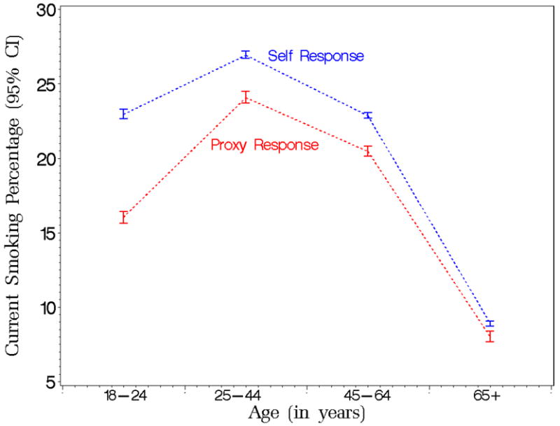
Smoking prevalence predicted marginals with 95% confidence limits by age and respondent type from the Tobacco Use Supplement to the Current Population Survey (TUS-CPS) for the period 1992 to 2003.

A detailed description of the CPS design and data collection process is described in Current Population Survey (2006). Briefly, the first stage of sampling divides the United States into primary sampling units (PSUs), where a PSU corresponds to a metropolitan area, a large county, or a group of counties, so that every unit falls within a state boundary. The PSUs are grouped into strata that are as homogeneous as possible in terms of characteristics highly related to unemployment – based on independent information obtained from decennial census and other sources. One PSU is chosen from each stratum with a selection probability proportional to its population. The PSUs remain constant between CPS redesigns, which occur every 10 years following the decennial U.S. Census. The 1980 CPS-design began in January 1985 and included 792 PSUs; the 1990 CPS-design began on April 1994 with 729 PSUs.

In the second stage of the CPS, housing units (which are combined into small groups, or ultimate sampling units (USUs) are selected within the sample PSUs. The USUs are defined so that they represent housing units from blocks with similar demographic composition and geographic proximity.

The Current Population Survey presents a detailed explanation how the statistical weights are constructed for the CPS core, Current Population Survey (2006, Chapter 10), and describes the weighting method for supplements such as the TUS-CPS, Current Population Survey (2006, Chapter 11). Briefly, each TUS-CPS monthly sample is nationally representative of the civilian non-institutionalized population of the United States and weighted to represent the population for that year. The weighting is a multi-stage process to adjust for differential selection probabilities, non-response and non-coverage. When the 3 months are combined for any given wave, their weights are divided by three so that they represent the population for that year. As illustrated in Table 1a, each TUS-CPS wave yields between 233,297 and 271,490 respondents with a total sample size of 1,196,680.

Table 1.

a: Sample counts by sex, TUS-CPS, 1992-2003

Survey Year	Males	Females	Total
1992-93	125,172	146,308	271,480
1995-96	107,314	125,983	233,297
1998-99	105,010	119,499	224,509
2001-02	109,808	124,030	233,838
2003	109,686	123,870	233,556
Total	556,990	639,690	1,196,680

b: Sample counts by sex for survey attributes, TUS-CPS, 1992-2003
	Males		Females
	Sample Size	Percent	Sample Size	Percent
Survey Mode
Telephone	390,507	70.1	447,299	69.9
Personal visit	166,483	29.9	192,391	30.1
Respondent Type
Proxy	146,487	26.3	96,009	15.0
Self	410,503	73.7	543,681	85.0

To assess the current smoking prevalence in the adult population (age 18 years and older) we used the definition of current smoking status given in the Current Population Survey: Tobacco Use Supplement (2006, Section A), which is presented in Appendix 2. In this a person is defined as a current smoker if he/she had smoked at least 100 cigarettes in his/her lifetime and was smoking every day or some days at the time of a survey. In addition, we considered individual-level demographic characteristics that might affect smoking prevalence, such as age, race/ethnicity, sex, employment status and education; family-level demographic characteristics such as metropolitan status and region; and survey year, survey mode, and respondent type. All of the individual-level and family-level characteristics were obtained from the CPS Core and survey year, survey mode, and respondent type data came from the TUS-CPS.

Appendix 3 presents the weighted counts and population sizes by individual-level demographic characteristics. To adjust for different coding of race/ethnicity that was instituted in 2003, Bowles et al. (2003), we use five multiply imputed, see Rubin (1987), race/ethnicity values for responders of multiple race/ethnicities, see Davis et al. (2007).

The TUS-CPS survey allows both self- and proxy-responses for questions determining current smoking status. The TUS-CPS interviewer is instructed to only interview a proxy-respondent if this is the 4th callback, the person will not return before closeout of the 8-10 day interview period, or the responder is becoming irritated. The analyses conducted here include information from both self- and proxy-respondents, who were at least age 18 years at the time of a survey. In a case of a self-response, sex, age, and education correspond to the respondent himself or herself. In a case of a proxy-response, these demographic characteristics correspond to the person whose current smoking status is being reported by the proxy-respondent.

Table 1b shows that a much higher rate of proxy-responses was observed for males (26.3%) than for females (15.0%). The table also shows that approximately 30% of the TUS-CPS responses were obtained in-person for both sexes.

The overall TUS-CPS response rate can be summarized using both the CPS Core response rate (a household response rate) and the TUS “conditional” response rate, which is computed as the fraction of those individuals who completed the TUS-CPS to those who completed the CPS, e.g., Current Population Survey: Tobacco Use Supplement (2006). The CPS Core “yearly” response rates range from 92.7% in 2003 to 95.4% in 1992-1993, with an average of 93.5%. The TUS-CPS conditional response rates for the five yearly surveys were 88.0%, 86.2%, 84.8%, 82.8%, and 83.0% for 1992-93, 1995-96, 1998-99, 2001-02, and 2003, respectively, for those age 18 years and older, with an average of 84.9%.

2.2 Data Analysis

We use SAS callable SUDAAN version 9.0.1 developed by the Research Triangle Institute (2004) running on a Sun server. These are single threaded applications so that they can take advantage of only one central processing unit. Our findings are based on a multiple logistic regression model of current smoking probability while controlling for survey attributes as well as demographic characteristics, such as all survey attributes, age, sex, race/ethnicity, education, employment status and region. In addition the analysis included six two-way interactions of survey mode with age, sex, and survey year and of respondent type with age, sex, and education. We obtained valid standard errors for the complex stratified CPS design by incorporating the TUS-CPS replicate weights described below.

Replication methods are used to provide variance estimates for a wide variety of designs including probability sampling even when complex estimation procedures are used, see Wolter (2007). The Current Population Survey uses the Balanced Repeated Replication (BRR) method to derive replication weights. Random subsamples are drawn from the full sample and these subsamples are called replicates. The derivation of the CPS replication weights and their use in variance estimation is described completely in the Current Population Survey (2006, Chapter 14). Beginning with the 1980 CPS, design replication weights were derived using a balanced half-sample approach. Each replicate retains all features of the sample design, such as the stratification and the within-PSU sample selection. The 1980 CPS design used 48 replicates and the 1990 design used 80 replicates. Appendix 4 describes this method in detail.

Initially, we examined all main effects presented in Appendix 3. However, metropolitan status was identified as a non-significant predictor of current smoking status and thus, was not included in the final model. The run-time of the final model was approximately 24 hours.

3 Results

In this section we present the results of our multiple logistic regression model discussed in Section 2.2. We state the conclusions in terms of the overall significance of each covariate based on Wald’s test and post-hoc comparisons with Bonferroni adjustments for multiple testing, proposed by Fisher (1935). All statistically significant differences are illustrated in Tables 2 and 3. These tables also define the reference groups used in the analysis. The intercept, all main effects except for survey mode (p-value is 0.675), and all interaction terms are significant at 5% level (p-values are less than 0.0001). The prediction results are presented in terms of the predicted marginals, discussed by Korn and Graubard (1999), with the corresponding 95% confidence intervals for current smoking prevalence. Some of the prediction results are illustrated in Figures 1-4.

Table 2.

Estimated odds ratios with 95% confidence intervals for interactions

	Predictor	Odds Ratio
Sex, Respondent Type (Reference Group: Female and Male, Self)
	Male, Proxy	1.23* (1.20, 1.27)
Age, Respondent Type (Reference Group: Self and 65+, Proxy)
	18-24, Proxy	0.71* (0.66, 0.75)
	25-44, Proxy	0.97 (0.92, 1.02)
	45-64, Proxy	0.98 (0.93, 1.03)
Education, Respondent Type (Reference Group: Self and 16+, Proxy)
	< 12 years, Proxy	0.97 (0.92, 1.03)
	12 years, Proxy	1.07* (1.02, 1.12)
	13-15 years, Proxy	0.92* (0.88, 0.96)
Survey Year, Survey Mode (Reference Group: In-Person and 2003, Telephone)
	1992-93, Telephone	0.90* (0.86, 0.94)
	1995-96, Telephone	0.95 (0.91, 1.00)
	1998-99, Telephone	0.92* (0.88, 0.96)
	2001-02, Telephone	0.96 (0.91, 1.00)
Sex, Survey Mode (Reference Group: Female and Male, In-Person)
	Male, Telephone	0.92* (0.90, 0.94)
Age, Survey Mode (Reference Group: In-Person and 65+, Telephone)
	18-24, Telephone	0.86* (0.81, 0.91)
	25-44, Telephone	0.90* (0.86. 0.93)
	45-64, Telephone	0.92* (0.87, 0.96)

Note: Results are based on logistic regression. Reference groups for interactions are determined based on the reference groups for the main effects presented in Table 2;

^*Indicates a statistically significant result when compared to the reference group at 5% significance level.

Table 3.

Estimated odds ratios with 95% confidence intervals for main effects

	Predictor	Odds Ratio
Individual-Level Demographic Characteristics
	Sex (Reference Group: Female)
	Male	1.38* (1.34, 1.40)
	Age (Reference Group: 65+)
	18-24	3.53* (3.39, 3.69)
	25-44	4.32* (4.17, 4.47)
	45-64	3.38* (3.25, 3.61)
	Education (Reference Group: 16+ years)
	< 12 years	4.84* (4.72, 4.97)
	12 years	3.51* (3.43, 3.58)
	13-15 years	2.51* (2.46, 2.56)
	Race/Ethnicity (Reference Group: Non-Hispanic White)
	Non-Hispanic Black	0.71* (0.69, 0.72)
	Non-Hispanic AIAN	1.39* (1.26, 1.54)
	Non-Hispanic API	0.55* (0.52, 0.57)
	Hispanic	0.40* (0.39, 0.41)
	Employment Status (Reference Group: Not in Labor Force)
	Employed	1.07* (1.05, 1.08)
	Unemployed	1.78* (1.73, 1.83)
Family-Level Demographic Characteristic
	Region (Reference Group: West)
	Northeast	1.07* (1.04, 1.10)
	Midwest	1.20* (1.18, 1.23)
	South	1.18* (1.15, 1.21)
Survey Attributes
	Survey Mode (Reference Group: Personal Visit) Telephone	1.01 (0.96, 1.06)
	Respondent Type (Reference Group: Self) Proxy	0.79* (0.74, 0.85)
Survey Year
	Survey Year (Reference Group: 2003)
	1992-93	1.36* (1.31, 1.41)
	1995-96	1.30* (1.25, 1.35)
	1998-99	1.25* (1.20, 1.30)
	2001-02	1.16* (1.12, 1.20)

Note: Results are based on logistic regression. Odds ratio of intercept is 0.02 with lower and upper limits of 0.02 and 0.03, respectively.

^*Indicates a statistically significant result when compared to the reference group at 5% significance level.

Figure 1.

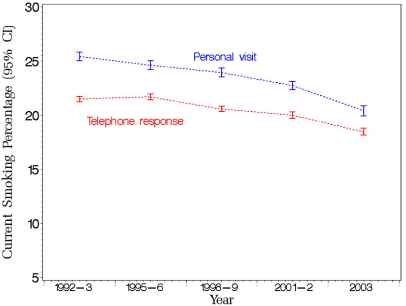
Smoking prevalence predicted marginals with 95% confidence limits by year and survey mode from the Tobacco Use Supplement to the Current Population Survey (TUS-CPS) for the period 1992 to 2003.

Figure 4.

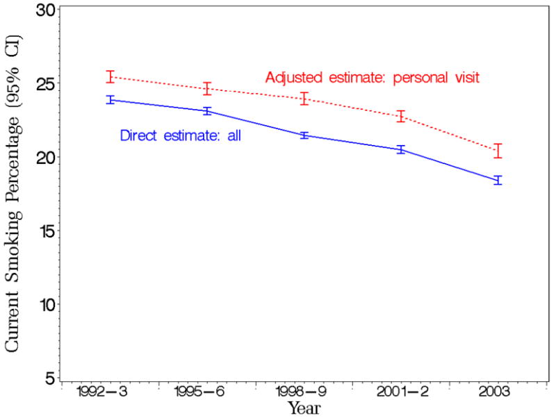
Smoking prevalence predicted marginal estimates with 95% confidence limits based on in-person interviews and overall direct estimates by survey year from the Tobacco Use Supplement to the Current Population Survey (TUS-CPS) for the period 1992 to 2003.

3.1 Interpretation of Interaction Terms

For current smoking prevalence, we found a significant interaction between survey mode and survey year. Figure 1 presents the detailed predicted marginal estimates with 95% confidence limits of current smoking trends by survey mode and survey year, with wider confidence intervals for estimates corresponding to the in-person interviews due to the smaller sample sizes associated with this mode. The figure indicates a decreasing difference between the mean estimates over time. As indicated in Table 2, a test of the interaction of survey mode with survey year shows a statistically significant difference in 1992-93 and 1998-99 (odds ratios are less than 1.00) compared to the reference group (both p-values are less than 0.0001).

As for the interaction of survey mode and sex, males who have a telephone interview are significantly different in terms of the current smoking prevalence than the other respondents (p-value is less than 0.0001). The predicted marginals of current smoking occurrence are given as 22% and 26% for males who have a telephone interview and an in-person interview, respectively, and as 18% and 20% for females who have a telephone interview and an in-person interview, respectively. We note that for each sex respondents who have the interview in-person tend to report a higher average smoking prevalence than respondents who have a telephone interview with a difference of 4% for males and 2% for females. This observation is further discussed in Section 4.

Figure 2 presents the predicted marginals of current smoking trends by survey mode and age group. It illustrates the larger survey mode prevalence difference for the three younger age groups (compared to the elderly). Because all p-values are less than 0.0001, we conclude that current smoking prevalence of people who are age 18 to 24, 25 to 44, or 45 to 64 years and have a telephone interview is different from the prevalence of the reference group, adjusting for other factors.

Figure 2.

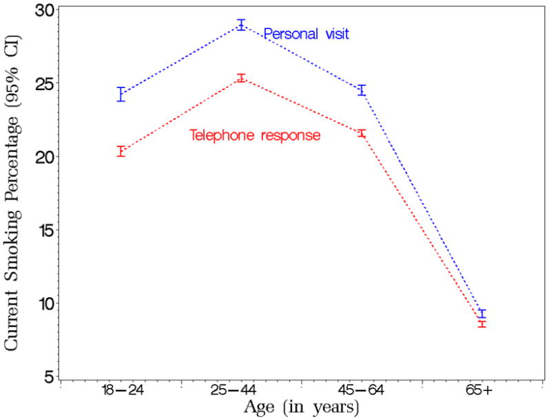
Smoking prevalence predicted marginals with 95% confidence limits by age and survey mode from the Tobacco Use Supplement to the Current Population Survey (TUS-CPS) for the period 1992 to 2003.

With respect to the interaction terms of respondent type with sex, we conclude that males with proxy-responses are different in terms of current smoking prevalence from the reference group (p-value is less than 0.0001). The predicted marginals are given by 23% for males with proxy-responses, 24% for male self-respondents, 16% for female with proxy-responses, and 20% for female self-respondents, with a larger difference for females (4%) than for males (1%) shown.

Figure 3 presents the predicted marginals of current smoking trends by respondent type and age group. The figure shows a decreasing gap between the prevalence differences with increasing age. Only one group, individuals age 18 to 24 years with proxy-responses, is significantly different in terms of the current smoking prevalence from the reference subpopulation (p-value is less than 0.0001).

With regard to the interaction between the respondent type and education, we conclude that people who have exactly 12 or 13 to 15 years of education and are reported by proxy-respondents are significantly different in terms of the current smoking from the reference population: the respective p-values are given by 0.008 and 0.0001. The corresponding predicted marginals of current smoking prevalence are 29% for people with less than 12 years of education with proxy-responses, 33% for self-respondents with less than 12 years of education, 25% for people with 12 years of education with proxy-responses, 27% for self-respondents with 12 years of education, 17% for people with 13-15 years of education with proxy-responses, 21% for self-respondents with 13-15 years of education, 8% for people with 16 or more years of education with proxy-responses and 10% for self-respondents with 16 or more years of education.

3.2 Interpretation of Key Main Terms

Table 3 presents estimated odds ratios with the corresponding 95% confidence intervals for all main effects. This table can be used together with Table 2 to draw additional conclusions, if needed. Below we discuss key main terms with respect to current smoking while controlling for other factors.

First, race/ethnicity is an important predictor of current smoking prevalence. In particular, Non-Hispanic American Indians and Alaska Natives are more likely to smoke than are Non-Hispanic Whites. Hispanics, Asians, and Blacks and are less likely to smoke than are Non-Hispanic Whites (all p-values are less than 0.0001).

Next, employment status is a significant predictor of smoking prevalence. Unemployed and employed people are more likely to currently smoke than people who are not in the labor force (p-values are less than 0.0001).

Finally, in terms of region where the respondents reside and the survey is conducted, the highest odds ratio of current smoking incidence corresponds to the Midwest and South, and followed by the Northeast. The three regions correspond to significantly different ratios than does the West (all p-values are less than 0.0001).

4 Discussion

The main goal of this study was to assess any possible differences in current smoking prevalence based on survey mode (in-person versus telephone interview) and respondent type (self versus proxy) while controlling for demographic characteristics. Our analysis used the TUS-CPS data from 1992 to 2003. The large sample size – more than 1.1 million responses – allowed us to carry out complex statistical analyses, including estimation of interactions. Thus, we investigated the magnitude of differences with respect to a number of sociodemographic groups with respect to self-proxy respondent type and survey administration mode while controlling for overall current smoking prevalence changes over time. We also compared our results with smaller North American and European studies that were designed to explicitly study survey mode and respondent type.

4.1 Survey Mode

Telephone and in-person interviews are the two data collection modes considered in this study. Although the magnitude of the difference of current smoking prevalence by survey mode varies by year, the adjusted current smoking prevalence obtained by in-person responses is 3.0% (3.2% unadjusted) larger than one obtained from telephone responses when averaged over the five survey waves between 1992-2003 (Figure 1). Simile et al. (2006) found a larger difference (4.2% unadjusted) in current smoking prevalence between these two survey modes using 2005 NHIS data. Even though structured guidelines determine the survey mode for the TUS-CPS and the NHIS, respondents have some flexibility in the choice of survey mode in both surveys. As a result, we cannot conclude whether the difference in smoking prevalence is due to the difference between the respondents themselves or to the mode per se (i.e., people will respond differently to two modes). However, the 2003 Canadian Community Health Study randomized subjects to survey modes, and the current smoking prevalence obtained by in-person interviews was 1.9% larger (unadjusted) than those obtained from telephone responses, Beland and St. Pierre (2008). Thus, our estimated difference for U.S. adults (3.2% unadjusted and 3.0% adjusted) is in the same direction but larger than that obtained for Canadian adults using a randomized design.

Based on the assumption that people are unlikely to over report their current smoking status, we assume that the “correct” response would be obtained by a self-report from a personal visit. Unfortunately, this is not always available due to constraints on time and money and a respondent’s schedule. However, under this assumption the overall direct (crude) smoking prevalence estimates obtained from the TUS-CPS and available on-line, National Cancer Institute (2007b), can be improved when considering the specific survey attributes.

Figure 4 illustrates the difference in predicted marginals of smoking prevalence that would have been obtained if all interviews were done in-person versus the commonly used overall direct estimates. The graphs illustrate the difference in these estimates by year with an average difference of about 2%. The figure shows that the direct estimates would underestimate the true current smoking prevalence in the population at any given time, and the underestimate remains relatively constant over time. After controlling for all available variables, the TUS-CPS current smoking prevalence is higher when the interview is done in-person than by telephone. This is consistent with previous results based on randomized experiments presented by Holbrook et al. (2003) that telephone respondents were more likely to present themselves in socially desirable ways than were face-to-face respondents.

In addition, although it appears that on average, current smoking prevalence is higher when the interview is done in-person than when it is conducted by telephone and it holds for both sexes, based on significant interaction between survey mode and sex, we conclude that the current smoking prevalence difference between the two modes is larger for males than for females. Similarly, although current smoking prevalence reported in-person appears higher than when reported by telephone for all age groups, a significant interaction for survey mode by age group results in larger differences for those age 18 to 44 years than for those who are 45 to 64 years old. This difference is even much more pronounced when comparing 18 to 44 year old people with those 65 years or older where the mode difference for the latter practically disappears.

4.2 Respondent Type

The conclusions reached in previous studies (using both self- and proxy-responses for the same individuals) concerning the use of proxy-responses in current smoking estimates are mixed. Two studies from the 1990s in North America, Gilpin et al. (1994) and Hyland et al. (1997), concluded that the impact of including proxy-responses was negligible in the estimation of the current smoking prevalence for the population. However, a more recent Dutch study discussed by Harakeh et al. (2006) showed rather large differences, especially for parents reporting their children’s current smoking. Thus, the use of proxy-responses would affect the overall smoking prevalence estimate, especially for younger age subgroups.

We found that proxy-responses result, on average, in lower smoking estimates than do self-responses (Figure 3). In addition, we found that the magnitude of the distinction between self- and proxy-reported current smoking prevalence differs with respect to the age of a person for whom the current smoking status is reported. This distinction is largest when the responses concern individuals age 18 to 24 years. This probably reflects the fact that many parents or guardians may assume incorrectly that their child is not smoking. These results are similar to those found by Harakeh et al. (2006).

4.3 Summary and Future Research

Although our findings could suggest using only self-responses and personal visits when assessing current smoking prevalence, this strategy would lead to substantial reduction of the sample size and thus, is not recommended by us. We suggest incorporating all self- and proxy-responses together with both survey administration modes provided that appropriate adjustments of estimates are made. These adjustments are important, especially when comparing survey results with results of surveys that use only self-response and with results based on other national surveys such as the NHIS. More generally, this information is crucial given that future surveillance is moving toward more complex designs, such as multiple mode and frame designs discussed by Brick and Lepkowski (2008), which will not only create dissimilarities between results based on different national and state surveys but can also create differences within a survey series.

The presented TUS-CPS data analysis suggests a number of additional future research questions. First, it would be useful for tobacco researchers to consider whether proxy-responses for current smoking should be allowed for those who are 18 to 24 years old; or, more generally, whether the TUS-CPS rules for elicitation of proxy-responses need to be modified. It also would be practical to study the relationship of the proxy-respondent to the person whose current smoking status is being reported.

Next, it would be of interest to consider three-way interactions of respondent type, survey mode and other covariates. In addition, the impact of other factors in the TUS-CPS data collection process, such as other types of survey interview (Computer-Assisted Telephone Interviewing, which is always done by a central telephone facility and Computer-Assisted Personal Interviewing, which is done either by telephone or in person by a field interviewer) are yet to be investigated. Including these and other factors might improve our understanding of longitudinal trajectories of current smoking prevalence. Also, it would be useful to find out whether some randomized studies or re-interview type studies would confirm the possible survey attribute effects seen here. At a minimum, national and state surveys should provide the necessary information so that investigators can study and correct for possible survey and respondent type biases.

Appendix 1: TUS-CPS rotation chart for 1998-1999

	Sample Number/Rotation Group
Year/Month	A72	A73	A74	A75	A76
1998
JAN	- - 3 4 5 6 - -	- - - - - - 7 8	1 2
FEB	- - - 4 5 6 7 -	- - - - - - - 8	1 2 3
MAR	- - - - 5 6 7 8	- - - - - - - -	1 2 3 4
APR	- - - - - 6 7 8	1 - - - - - - -	- 2 3 4 5
MAY	- - - - - - 7 8	1 2 - - - - - -
JUNE	- - - - - - - 8	1 2 3 - - - - -
JULY	- - - - - - - -	1 2 3 4 - - - -
AUG	- - - - - - - -	- 2 3 4 5 - - -	1
SEPT	- - - - - - - -	- - 3 4 5 6 - -	- - - - - - 7 8	1 2
OCT	- - - - - - - -	- - - 4 5 6 7 -	- - - - - - - 8	1 2 3
NOV	- - - - - - - -	- - - 5 6 7 8 -	- - - - - - - -	1 2 3 4
DEC	- - - - - - - -	- - - - 6 7 8 -	1 - - - - - - -	- 2 3 4 5
1999
JAN	- - - - - - - -	- - - - - - 7 8	1 2 - - - - - -	- - 3 4 5 6
FEB	- - - - - - - -	- - - - - - - 8	1 2 3 - - - - -	- - - 4 5 6 7
MAR	- - - - - - - -	- - - - - - - -	1 2 3 4 - - - -	- - - - 5 6 7 8
APR	- - - - - - - -	- - - - - - - -	- 2 3 4 5 - - -	- - - - - 6 7 8	1
MAY	- - - - - - - -	- - - - - - - -	- - 3 4 5 6 - -	- - - - - - 7 8	1 2
JUNE	- - - - - - - -	- - - - - - - -	- - - 4 5 6 7 -	- - - - - - - 8	1 2 3
JULY	- - - - - - - -	- - - - - - - -	- - - - 5 6 7 8	- - - - - - - -	1 2 3 4
AUG	- - - - - - - -	- - - - - - - -	- - - - - 6 7 8	1 - - - - - - -	- 2 3 4 5
SEPT	- - - - - - - -	- - - - - - - -	- - - - - - 7 8	1 2 - - - - - -	- - 3 4 5 6
OCT	- - - - - - - -	- - - - - - - -	- - - - - - - 8	1 2 3 - - - - -	- - - 4 5 6 7
NOV	- - - - - - - -	- - - - - - - -	- - - - - - - -	1 2 3 4 - - - -	- - - - 5 6 7 8

Note: This is an adapted version of CPS rotation chart for 1998 and 1999 demonstrating the TUS-CPS 1998-1999 yearly sample. The sample and rotation groups for the TUS-CPS sample months (September 1998, January 1999, and May 1999) are bolded. The rotation chart shows when to interview the sample units for a particular sample designation and rotation. A sample designation is represented by the letter “A” and a two-digit number. Each sample designation consists of rotations numbered 1 through 8. Each month, a new sample/rotation comes into sample for the first time, and another sample/rotation returns to sample after an eight-month lapse. Figure shows that the 24 sample/rotation groups introduced “between” A73 group 3 and A76 group 2 were in sample exactly once in these 3 TUS-CPS monthly samples – demonstrating the efficiency of selecting every fourth month.

Appendix 2: TUS-CPS smoking question used to determine current smoking status

• Q1. (Have/Has) (you/ name) smoked at least 100 cigarettes in (your/his/her) entire life?

  • (1)Yes (continue)
  • (2)No (skip to next section)

  • Don’t Know OR Refused: (skip to next section)

• Q2. (Do/Does) (you/name) now smoke cigarettes every day, some days, or not at all?

  1. Every day

  2. Some days

  3. Not at all

Anyone answering “Yes” to Q1 and (1) or (2) to Q2 is a current smoker while all others are not current smokers.

Appendix 3: Demographic characteristics of TUS-CPS sample

	Males			Females
	Sample Size	Population	Percent*	Sample Size	Population	Percent*
Age
18-24	65,883	12,764,465	13.6	71,238	12,928,953	12.6
25-44	232,188	40,078,888	42.6	256,103	41,533,268	40.5
45-64	171,391	27,422,735	29.5	187,961	29,702,365	28.9
65+	87,528	13,459,003	14.3	124,388	18,487,364	18.0
Education
< 12 years	94,523	16,581,967	17.6	106,647	17,677,620	17.2
12 years	179,765	29,666,898	31.6	220,322	34,572,514	33.7
13-15 years	141,359	24,039,306	25.6	174,907	28,139,319	27.4
16+ years	141,343	23,736,919	25.2	137,814	22,262,497	21.7
Race/Ethnicity
Non-Hispanic Black	43,575	9,831,786	10.5	63,214	12,397,674	12.1
Non-Hispanic AIAN	5,715	645,272	0.7	6,631	715,362	0.7
Non-Hispanic API	18,903	3,419,817	3.6	21,961	3,841,155	3.7
Hispanic	45,487	10,160,542	10.8	49,721	10,190,060	9.9
Non-Hispanic White	443,309	69,967,675	74.4	498,163	75,507,699	73.6
Employment Status
Employed	400,668	67,984,012	72.3	365,177	58,711,744	57.2
Unemployed	22,781	4,098,018	4.4	19,948	3,441,245	3.4
Not in Labor Force	133,541	21,943,061	23.3	254,565	40,498,960	39.5
Metropolitan Status
Metropolitan	410,059	75,345,494	80.1	474,792	82,490,277	80.4
Non Metropolitan	143,145	18,361,803	19.5	160,702	19,828,595	19.3
Not Identified	3,786	317,795	0.3	4,196	333,078	0.3
Region
Northeast	122,437	18,164,626	19.3	143,541	20,315,401	19.8
Midwest	138,300	21,522,618	23.2	156,868	23,687,423	23.1
South	163,820	32,922,205	35.0	193,465	36,455,570	35.5
West	132,433	21,115,643	22.5	145,816	22,193,555	21.6

^*Percentages are based on populations and may not sum to 100% due to rounding; AIAN and API stand for American Indian and Alaska Native and Asian and Pacific Islander, respectively

Appendix 4: On balanced repeated replication

In general the balanced repeated replication method (BRR) retains about one-half of the sample. It is most easily explained for a design with S strata and 2 PSUs per strata. A single PSU can be selected from each strata in 2^S ways. However, all of the information in the replicates is available in g orthogonal or “balanced” replications. The CPS uses Fay’s (1984) generalized replication method, a variant of the BRR method to generate replicate weights and to estimate variance, see Lent (1991). In the CPS, for any of the g orthogonal replicates the sampling weights in the selected half sample are multiplied by 1.5 while the remaining weights are multiplied by 0.5, see Judkins (1990) for justification of the 1.5 and 0.5. Then the variance is computed using

$$\widehat{\mathit{Var}}(\widehat{\eta })=\frac{4}{g}\sum _{i=1}^g{({\widehat{\eta }}_{[i]}-\widehat{\eta })}^2$$

where η̂_[i] the estimate using the ith replication (i = 1, .., g) and η̂ is the full-sample estimator. The main advantage of the BRR when compared to other variance estimation methods is that it results in variance estimate that is asymptotically equivalent to that from Taylor’s linearization method for some functions of parameters. While the BRR method can be computationally intensive, it does not require as much computing as jackknife or bootstrap approaches, see Lohr (1999).

References

- Beland Y, St-Pierre M. Mode Effects in the Canadian Community Health Survey: A Comparison of CAPI and CATI. In: J ML, et al., editors. Advances in Telephone Survey Methodology. New York: John Wiley & Sons; 2008. pp. 297–316. [Google Scholar]
- Biener L, Garrett CA, Gilpin EA, Roman AM, Currivan DB. Consequences of declining survey response rates for smoking prevalence estimates. American Journal of Preventive Medicine. 2004;27:254–257. doi: 10.1016/j.amepre.2004.05.006. [DOI] [PubMed] [Google Scholar]
- Bowles M, Ilg RE, Miller S, Robison E, Polivka A. Revisions to the Current Population Survey effective in January 2003. Employment and Earnings; 2003. [Google Scholar]
- Brick JM, Lepkowski JM. Multiple mode and frame telephone surveys. In: J ML, et al., editors. Advances in Telephone Survey Methodology. New York: John Wiley & Sons; 2008. pp. 149–169. [Google Scholar]
- Caraballo RS, Giovino GA, Pechacek TF, Mowery PD. Factors associated with discrepancies between self-reports on cigarette smoking and measured serum cotinine levels among persons aged 17 years and older. American Journal of Epidemiology. 2001;153:807–814. doi: 10.1093/aje/153.8.807. [DOI] [PubMed] [Google Scholar]
- Centers for Disease Control and Prevention. Annual smoking-attributable mortality, years of potential life lost, and economic costs - United States, 1995-1999. Morbidity and Mortality Weekly Report. 2002;51(14):300–303. [PubMed] [Google Scholar]
- Centers for Disease Control and Prevention. Percentage of adults who were current, former, or never smokers, overall and by sex, race, Hispanic origin, age, education, and poverty status. 2008 http://www.cdc.gov/tobacco/data_statistics/tables/adult/table_2.html.
- Current Population Survey. U S Census Bureau. Current Population Survey: Design and Methodology. 2006 Technical Paper 66, http://www.census.gov/prod/2006pubs/tp-66.pdf.
- Current Population Survey: Tobacco Use Supplement. Technical Documentation CPS-03 Attachment 16 Source and Accuracy of the February, June and November 2003 Tobacco Use Supplement Data. 2006 http://riskfactor.cancer.gov/studies/tus-cps/surveys/cps_fjn03_tech_doc.pdf.
- Davis WW, Hartman AM, Gibson JT. Bridging estimates by race for the Tobacco Use Supplement to the Current Population Survey. 2007 http://riskfactor.cancer.gov/studies/tus-cps/race_bridging_071307.pdf.
- De Leeuw ED. To mix or not to mix data collection modes in surveys. Journal of Offcial Statistics. 2005;21:233–255. [Google Scholar]
- Fagan P, Shavers V, Lawrence D, Gibson JT, Ponder P. Cigarette smoking and quitting behaviors among unemployed adults in the United States. Nicotine and Tobacco Research. 2007;9(2):241–248. doi: 10.1080/14622200601080331. [DOI] [PubMed] [Google Scholar]
- Fay RE. Some properties of estimates of variance based on replication methods; Proceedings of the Survey Research Methods; American Statistical Association; 1984. pp. 495–500. [Google Scholar]
- Fisher RA. Statistical Tests. Nature. 1935;136:474–475. [Google Scholar]
- Gilpin EA, Pierce JP, Cavin SW, Berry CC, Evans NJ, Johnson M, et al. Estimates of population smoking prevalence: self- vs proxy reports of smoking status. American Journal of Public Health. 1994;84(10):1576–1579. doi: 10.2105/ajph.84.10.1576. [DOI] [PMC free article] [PubMed] [Google Scholar]
- Green MP, McCausland KL, Xiao H, Duke JC, Vallone DM, Healton CG. A closer look at smoking among young adults: where tobacco control should focus its attention. American Journal of Public Health. 2007;97(8):1427–1433. doi: 10.2105/AJPH.2006.103945. [DOI] [PMC free article] [PubMed] [Google Scholar]
- Groves RM, Miller PV, Cannell CF. Vital and Health Statistics. 106. Vol. 2. Hyattsville, MD: DHHS; 1987. An Experimental Comparison of Telephone and Personal Interview Surveys; pp. 11–19. [PubMed] [Google Scholar]
- Harakeh Z, Engels R, De Vries H, Scolte RDJ. Correspondence between proxy and self-reports on smoking in a full family study. Drug and Alcohol Dependence. 2006;84(1):40–47. doi: 10.1016/j.drugalcdep.2005.11.026. [DOI] [PubMed] [Google Scholar]
- Holbrook AL, Green MC, Krosnick JA. Telephone versus face-to-face interviewing of national probability samples with long questionnaires: comparisons of respondent satisficing and social desirability response bias. Public Opinion Quarterly. 2003;67:79–125. [Google Scholar]
- Hyland A, Cummings KM, Lynn WR, Corle D, Giffen CA. Effect of proxy-reported smoking statust of population estimates of smoking prevalence. American Journal of Epidemiology. 1997;145(8):746–751. doi: 10.1093/aje/145.8.746. [DOI] [PubMed] [Google Scholar]
- Judkins DR. Fay’s Method for Variance Estimation. Journal of Official Statistics. 1990;6:223–239. [Google Scholar]
- Korn EL, Graubard BI. Analysis of Health Surveys. New York: John Wiley & Sons; 1999. [Google Scholar]
- Lent J. Variance estimation for Current Population survey small area labor force estimates; Proceedings of the Survey Research Methods; American Statistical Association; 1991. pp. 11–20. [Google Scholar]
- Lohr SL. Sampling: Design and Analysis. Pacific Grove: Brooks/Cole Publishing Company; 1999. [Google Scholar]
- National Cancer Institute. Tobacco Use Supplement; Current Population Survey Reports and Publications using the TUS-CPS. 2007a http://riskfactor.cancer.gov/studies/tus-cps/publications.html.
- National Cancer Institute. Tobacco Use Supplement; Current Population Survey What are the Current and Past TUS Survey Findings? 2007b http://riskfactor.cancer.gov/studies/tus-cps/results.html.
- National Cancer Institute. U S Department of Commerce, Census Bureau National Cancer Institute Sponsored Tobacco Use Supplement to the Current Population Survey. 2007c http://riskfactor.cancer.gov/studies/tus-cps.
- Navarro A. Smoking status by proxy and self report: rate of agreement in different ethnic groups. Tobacco Control. 1999;8:182–185. doi: 10.1136/tc.8.2.182. [DOI] [PMC free article] [PubMed] [Google Scholar]
- Patrick DL, Cheadle A, Thompson DC, Diehr P, Koepsell T, Kinne S. The validity of self-reported smoking: a review and meta-analysis. American Journal of Public Health. 1994;84:1086–1093. doi: 10.2105/ajph.84.7.1086. [DOI] [PMC free article] [PubMed] [Google Scholar]
- Pleis JR, Lethbridge-Çejku M. Summary health statistics for U.S. adults: National Health Interview Survey, 2006. National Center for Health Statistics. Vital Health Statistics. 2007;10(235) [PubMed] [Google Scholar]
- Research Triangle Institute. SUDAAN Language Manual, Release 9.0. Research Triangle Park, NC: Research Triangle Institute; 2004. [Google Scholar]
- Rubin DB. Multiple imputation for nonresponse in Surveys. New York: John Wiley & Sons; 1987. [Google Scholar]
- Shavers V, Lawrence D, Fagan F, Gibson JM. Racial/ethnic variation in cigarette smoking among the civilian U.S. population by occupation and industry, TUS-CPS 1998-1999. Preventive Medicine. 2005;41:597–606. doi: 10.1016/j.ypmed.2004.12.004. [DOI] [PubMed] [Google Scholar]
- Simile CM, Stussman B, Dahlhamer JM. Exploring the impact of mode on key health estimates in the National Health Interview Survey; Proceedings of Statistics Canada Symposium 2006: Methodological Issues in Measuring Population Health; 2006. http://www.fcsm.gov/07papers/Stussman.III-C.pdf. [Google Scholar]
- St-Pierre M, Beland Y. Mode Effects in the Canadian Community Health Survey: A Comparison of CAPI and CATI, 2004; Proceedings of the American Statistical Association Meeting, Survey Research Methods Section, Toronto; 2004. http://www.amstat.org/sections/srms/Proceedings/ [Google Scholar]
- Sudman S, Bradburn NM, Schwarz N. Thinking About Answers: The Application of Cognitive Processes to Survey Methodology. San Francisco: Jossey-Bass Publishers; 1996. [Google Scholar]
- Todorov A. Cognitive procedures for correcting proxy-response biases in surveys. Applied Cognitive Psychology. 2003;17:215–224. [Google Scholar]
- U.S. Department of Health and Human Services. The Health Consequences of Smoking: A Report of the Surgeon General. Atlanta, GA: 2004. U.S. http://www.cdc.gov/tobacco/data_statistics/sgr/sgr_2004/chapters.htm. [Google Scholar]
- U.S. Department of Health, Education, and Welfare. Smoking and Health: Report of the Advisory Committee to the Surgeon General of the Public Health Service. Washington: U.S. Department of Health, Education, and Welfare, Public Health Service, Center for Disease Control, 1964; 1964. HS Publication No. 1103. [Google Scholar]
- Wolter K. Introduction to Variance Estimation. 2. New York: Springer-Verlag; 2007. [Google Scholar]